Article

A Machine Learning Approach to Predicting the Turbidity from Filters in a Water Treatment Plant

by
Joseph Kwarko-Kyei
*,
Hoese Michel Tornyeviadzi
and
Razak Seidu
Smart Water Lab, Department of Ocean Operations and Civil Engineering, Norwegian University of Science and Technology (NTNU), 6009 Ålesund, Norway
*
Author to whom correspondence should be addressed.
Water 2025, 17(20), 2938; https://doi.org/10.3390/w17202938 (registering DOI)
Submission received: 8 September 2025 / Revised: 2 October 2025 / Accepted: 9 October 2025 / Published: 12 October 2025

Abstract

Rapid sand filtration is a critical step in the water treatment process, as its effectiveness directly impacts the supply of safe drinking water. However, optimising filtration processes in water treatment plants (WTPs) presents a significant challenge due to the varying operational parameters and conditions. This study applies explainable machine learning to enhance insights into predicting direct filtration operations at the Ålesund WTP in Norway. Three baseline models (Multiple Linear Regression, Support Vector Regression, and K-Nearest Neighbour (KNN)) and three ensemble models (Random Forest (RF), Extra Trees (ET), and XGBoost) were optimised using the GridSearchCV algorithm and implemented on seven filter units to predict their filtered water turbidity. The results indicate that ML models can reliably predict filtered water turbidity in WTPs, with Extra Trees models achieving the highest predictive performance (R2 = 0.92). ET, RF, and KNN ranked as the three top-performing models using Alternative Technique for Order of Preference by Similarity to Ideal Solution (A-TOPSIS) ranking for the suite of algorithms used. The feature importance analysis ranked the filter runtime, flow rate, and bed level. SHAP interpretation of the best model provided actionable insights, revealing how operational adjustments during the ripening stage can help mitigate filter breakthroughs. These findings offer valuable guidance for plant operators and highlight the benefits of explainable machine learning in water quality management.

1. Introduction

Water treatment plants are under increasing stress from increasing levels of contaminants of public health significance in their raw water sources due to climate-induced runoffs and increasing anthropogenic activities in their catchment areas [1]. Removing these contaminants to safeguard public health requires cost-effective drinking water treatment processes. Granular filtration is an important step in all water treatment plants and plays a critical role in the removal of chemical and microbial contaminants of public health concern [2]. Depending on the media properties, granular media filters also play the role of adjusting/correcting physicochemical parameters such as pH, colour, odour, and taste. The contaminant removal process involved in granular media filtration includes straining larger particles from the raw water and adsorption and/or precipitation of dissolved heavy metals by redox reactions. It also includes removal mechanisms such as interception, sedimentation, and the Brownian motion of particles within the flow streamlines. Particle dynamics, such as deposition kinetics [3] and particle detachment mechanisms impacted by hydraulic gradients and backwashing [4], were investigated in early research on granular media filtration. Turbidity monitoring has been pivotal in understanding filter performance, detecting particle breakthroughs, and optimising water treatment processes [5].
Hendricks, Clunie William [6] demonstrated that turbidity measurements are useful for assessing filter performance and for monitoring particle retention and microbial releases during filtration in rapid sand filters. Due to the dynamic nature of rapid filter behaviour, particularly during ripening and breakthrough, short-term turbidity fluctuation may indicate an increased risk of microbial breakthrough. Guideline values for filtered water turbidity, ranging from 1 to 2 NTU, are recommended. For example, certain Drinking Water Treatment Plant (DWTP) configurations require turbidity below 1 NTU after settling and coagulation-flocculation steps [7]. However, modern best practices recommend a stricter target of ≤0.1 NTU to minimise the risk of pathogen breakthroughs [8]. These developments have been accompanied by a regulatory shift towards mandatory continuous turbidity measurements using in-line sensors for plant capacities exceeding 10,000 m3/day, thereby enabling real-time operational oversight with Supervisory Control and Data Acquisition (SCADA) systems.
Filter operations play a critical role in maintaining water quality. For instance, during the backwash recovery (ripening) period, the recommended duration is under 15 min. If turbidity exceeds the safe limits, operators can intervene with corrective measures such as: (i) starting the filter slowly, (ii) delaying filtration, (iii) filtering to waste, or (iv) adding coagulation to the setup to aid the filtration process. Post-ripening, filtered water quality typically stabilises, but turbidity spikes during the breakthrough phase ultimately necessitate ending the filter cycle [8].
Drinking water treatment plants must also account for dynamic influent conditions, operational variability, and confounding external effects. Confounding effects of holidays, day-of-week effects, seasons, temperature and precipitation have been documented by Hsieh, Nguyen [9]. For optimal operation of granular filters, understanding the dynamics of breakthrough and the impact on turbidity in filtered water is critical. A key tool for managing turbidity is the filter breakthrough curves theory, which helps to predict particle breakthrough based on headloss progression during filtration. Therefore, by monitoring filter headloss, the filters can be isolated by valve action and backwashed before the breakthrough occurs. In other cases, the filter runtime is set to a limit beyond which the breakthrough is anticipated, considering the raw water quality and operation settings, without directly being triggered by the headloss [10,11].
With the increasing availability of treatment plant data, data-driven methods, particularly machine learning (ML) are increasingly applied to optimise particle removal in filtration systems. Various studies leverage ML algorithms, such as Artificial Neural Networks (ANNs), Decision Trees (DTs), Random Forests (RFs), Extreme Gradient Boosting (XGBoost), and Improved Random Forest (IRF), which have been successfully implemented to predict the efficiency of nanofiltration, membrane filtration, and rapid sand filtration in water treatment plants [12,13,14]. These models enhance operational decision-making by identifying patterns in turbidity, headloss, and breakthrough behaviour, ultimately improving filter performance [12,15,16]. However, a key limitation of existing models is that they typically treat filters in isolation, overlooking the variability between filters and the operational interdependencies among them. This is a critical gap, as full-scale drinking water treatment plants operate with multiple filters whose performance is interconnected [17,18]. This study addresses this gap by introducing models that capture the variabilities and interdependencies of multiple filters in a real-life treatment plant.
The primary objective of this study is to apply machine learning (ML) techniques to predict filtered water turbidity in a drinking water treatment plant in Ålesund, Norway. By exploring these predictive insights and accounting for operational factors, this study aims to optimise filter operation parameters, thereby enhancing water quality and operational efficiency. Additionally, we explore how data-driven decision-making can improve plant resilience and resource management, contributing to the broader digital transformation of water treatment systems.
This study is organised as follows: Section 1 presents the introduction; Section 2 details the methodology used, including a description of the case study plant and the framework for implementing machine learning (ML) models. Section 3 presents the results and discussion, incorporating SHapley Additive exPlanations (SHAP) analysis of ML models’ interpretability along with the study’s broader implications. Finally, Section 4 provides the conclusions and suggests directions for future research.

2. Materials and Methods

2.1. Overview of Drinking Water Treatment Plant

Figure 1 shows an overview of the drinking water treatment plant. The drinking water plant draws its raw water from Lake Brusdalsvatnet in Ålesund, a city on the coast of western Norway, with an annual rainfall of approximately 1830 mm [19], contributing to the dilution of dissolved organic matter (DOM) in surface water sources. According to the Norwegian water (Vann-Nett) classification, this lake has a high ecological and good chemical status [20]. Abstracted from a stable depth to the Ålesund waterworks, the treatment process involves dosing CO2 in-line to reduce the pH before chlorination. After this, the pre-treated water is passed through seven mono-media marble direct filters in a parallel arrangement. The combined effluent of the seven filter beds is redistributed to seven ultraviolet (UV) lamps for disinfection, which is collected in a clear water reservoir and transported to high-level reservoirs for distribution.
The inflow to the filter beds transitions to an open-channel flow with seven lateral-feeding manifolds with rectangular weir openings, which split to feed a gallery of seven in-house filters. The filters are housed to prevent freezing during winter and protect the influent water quality from deterioration. Each filter has a 20 m2 bed area, a 2 m depth, and a media effective diameter of 3 mm (L/d ratio = 666.7). A typical filter runtime is 7 days; therefore, a one-week backwashing cycle corresponds to filters 1–7 from Monday to Sunday. Backwashing involves pressurised air and clean water to fluidise the filter bed and flush trapped particles into the backwash trough. A typical backwashing duration is 15 ± 2 min. During backwash, the filter bed is isolated using the valves at both the inflow and outflow ends of the filter. The backwash water is collected into the backwash trough above the filter bed, retained, and later discharged into a local stream.
The filtration setup for this DWTP comprises marble sand media for pH correction and corrosion control for the water distribution network since the lake has a slightly lower pH (6.6–6.8), like most natural lakes in Norway, with low pH and low DOM in surface water. The filter serves as an auxiliary function for particle removal, which affects the turbidity of the raw water. Dissolved heavy metals in the raw water precipitate during a rapid pH drop during the pre-treatment stage and increase when they pass through the marble (CaCO3) media. The media is routinely replenished annually to maintain the bed level, which is affected by operational factors such as the total water filtered and the filter’s backwashing time. The backwashing process is initiated by shutting the outlet valve of the isolated filter. After closing the valve, pressurised air and clean water are flushed upwards to fluidise the filter bed, which enables trapped particles to float up and be collected by the backwashing trough.

2.2. Conceptual Framework of the Study

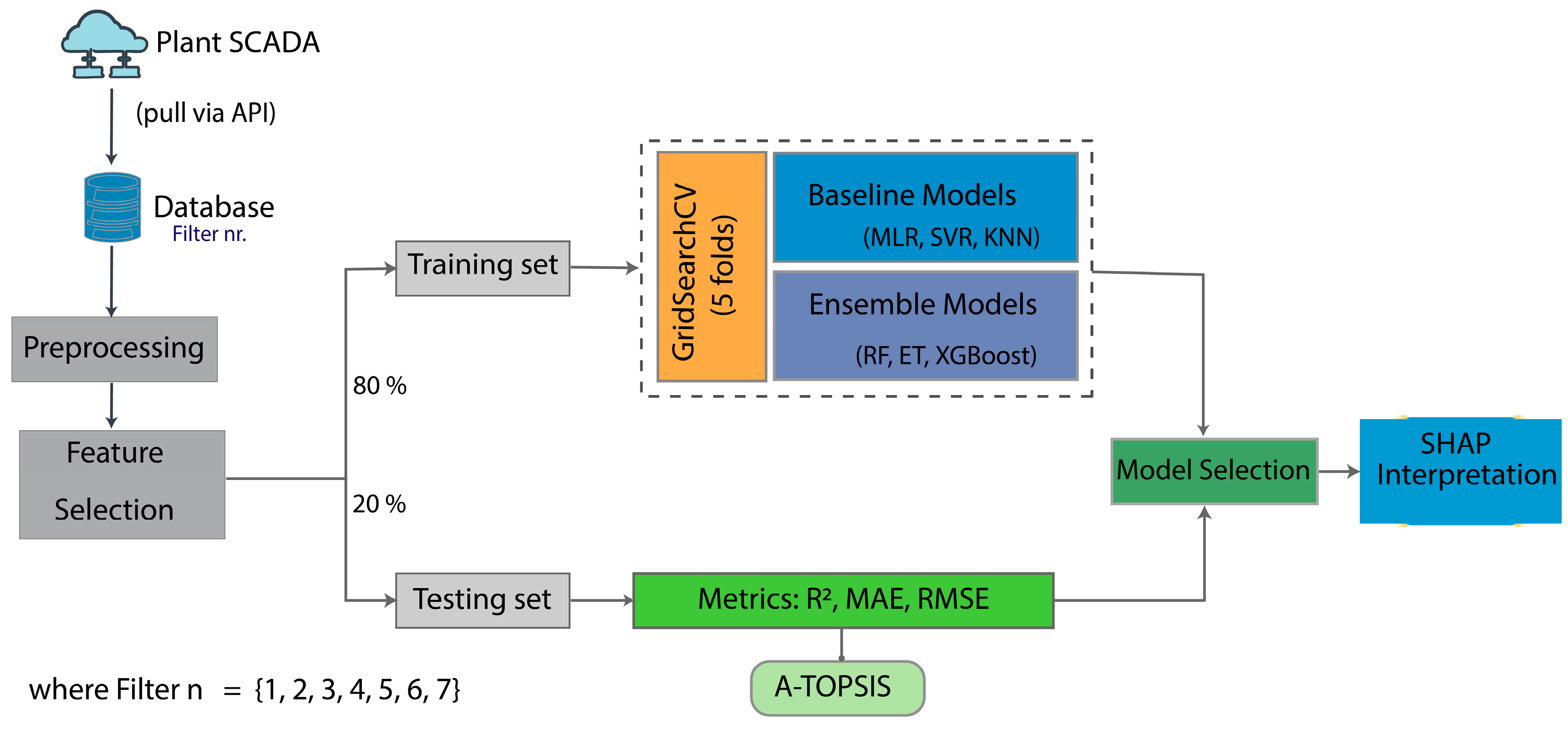
Figure 2 shows the conceptual framework adopted for ML development. The framework illustrates the workflow for developing and evaluating machine learning models to predict filtered water in DWTP filters. It comprises the interlinked steps of data collection and preprocessing from the plant, feature selection, model development and evaluation, and finally, model interpretation. These steps are elucidated in the sections below:

2.3. Data Collection, Structuring and Descriptive Analysis

The datasets for this study were collected from the Supervisory Control and Data Acquisition (SCADA) system via Application Programming Interface (API). Each data instance corresponds to a specific filter unit (Filter nr. ∈ [1, 2, 3, 4, 5, 6, 7]) within the Ålesund Drinking Water Treatment Plant. The study analysed four months (1 August 2023–1 December 2023) of high-resolution data (1 min interval) from the DWTP SCADA system, capturing valve opening (%), filtered water turbidity (NTU), flow rate (L/s), and bed level (m). This period was strategically selected to capture seasonal hydrodynamic effects, particularly lake upwelling and vertical mixing as predicted by the study lake’s hydrodynamic models [21], which have a marginal influence on the intake water quality at the abstraction point [22]. The filter runtime (in minutes) was derived from valve status (ON and OFF) and validated with the bed water level and operational reports. To assess the overall filtration performance, the combined filtered water turbidity from the gallery was computed as a flow-weighted average, providing a representative measure of treated water quality. Understanding the impact of unit filters on the collective system performance is essential for operational changes to optimise treatment efficiency. The Average Weighted Turbidity (AWT) at time t is computed using Equation (1) below.
A v e r a g e   W e i g h t e d   T u r b i d i t y =   i = 1 7 ( T i × Q i   ) i = 1 7 Q i
where T i is the turbidity of the f i l t e r i , and Q i is the flow rate (L/s) of the ith filter.

2.4. Machine Learning Models Development

2.4.1. Data Preprocessing and Feature Selection

The raw data preprocessing steps included imputation of missing values, where necessary. The NAN (Not a Number) turbidity readings, comprising 9.6% of the raw turbidity dataset, were addressed using the forward-fill imputation method. This method involves forward propagating the last valid observation to replace the missing values. These occurred intermittently, with a maximum of 20 consecutive rows affected during different time intervals as observed in a similar SCADA pattern [23]. The features selected for the machine learning models predicting the filtered water turbidity (NTU) of the individual filters were runtime (min.), flow (L/s), and level (m), based on operational relevance (validated by the plant manager) and supported by Pearson’s correlation. The valve opening (%) parameter was excluded from the input set to prevent data leakage, as it was directly used to derive the filter runtime data.
The machine learning models were developed to predict filtered water turbidity (NTU) for each individual filter using the following predictor variables: flow rate (L/s), bed level (m), and runtime (min). A total of 175,738 data rows were used for each filter, representing a monitoring period of 4 months. The dataset was partitioned into training (80%) and testing (20%) subsets for the machine learning models. The implementation and performance evaluation of the data-driven models are detailed in the subsequent sections.

2.4.2. Model Families and Evaluation

We evaluated a diverse suite of supervised machine learning model families to address the complexities and non-linearities of the DWTP filter datasets. These included three baseline models (Multiple Linear Regression (MLR), Support Vector Regression (SVR), K-Nearest Neighbours (KNN)) and three ensemble methods (Bagged Trees (Random Forest (RF) and Extra Trees (ET)) and Boosted Trees (Extreme Gradient Boosting (XGBoost))). All the features were pre-processed before model training to ensure optimal performance across the algorithm families. For baseline models that require scale-invariant comparisons, the features were standardised to have a zero mean and a unit variance scale using Scikit-learn’s StandardScaler (version 1.7.2). This preprocessing step is critical for: (i) enabling gradient-based optimisation in MLR, (ii) ensuring proper kernel weighting in SVR, and (iii) maintaining meaningful distance metrics in k-NN. In contrast, tree-based ensemble methods (Random Forest, Extra Trees, and XGBoost), which are generally insensitive to input feature scale, were trained on the raw feature values. The differential preprocessing approach was adopted to respect the mathematical assumptions of each algorithm family, as detailed below.
Baseline Models
Multiple Linear Regression (MLR)
Multiple linear regression (MLR) extends simple linear regression to model a continuous dependent variable and multiple independent variables. As a classical statistical technique widely used for predictive modelling, MLR models serve as foundational tools for supervised machine learning. MLR uniquely assumes no multicollinearity among independent variables in addition to the four key assumptions shared with simple linear regression models: linearity, independence of observations, homoscedasticity (constant variance of errors) and normally distributed residuals [24]. Although MLR is simple, it remains valuable for baseline studies and rapid prototyping. However, the technique performs poorly on non-linear relationships in real-world data. The general mathematical expression for the response variable, y and the independent variables is represented by:
y = β 0 + β 1 x n + + β n x n +   ε    
where β 0 is the intercept, β i denotes a coefficient that quantifies the change in response to a unit change in the independent variables, and ε   is the error term.
Support Vector Regression (SVR)
Support Vector Regression (SVR) is an adaptation of Support Vector Machines (SVMs), a robust class of supervised machine learning algorithms for handling both classification tasks and regression tasks. Unlike traditional regression methods that minimise error, SVR finds a function that deviates from the actual observed target within a specified margin (ε), while maintaining simplicity (flatness) [25].
In solving non-linear problems, the kernel functions (support vectors) map the data into a higher-dimensional space, where it becomes easier to fit an optimal hyperplane that captures the relationship between features and targets. The relationship between the predictors and predicted variables for an SVR can be mathematically expressed as
f x = i = 1 n ( α i α i * ) K x ,   x 1 + b        
where α i ,   α i * are Lagrange multipliers found during training, K x ,   x 1 is the kernel function user-defined, and b is the bias term [26]. The most popular kernels are the Radial Basis Function (RBF), polynomial, and sigmoid kernels; each is suited for various data complexities and structures as commonly implemented in scikit-learn.
K-Nearest Neighbour (KNN)
K-Nearest Neighbour (KNN) is a classical, non-parametric regression machine learning algorithm used for both regression and classification tasks. According to Györfi, Kohler [27], KNN is preferable for low-dimensional feature variables, as high-dimensional problems often lead to the curse of dimensionality. KNN predicts the target value for a query point x , by averaging the responses of its k nearest neighbours in the training set, based on a chosen distance metric (such as Euclidean or Manhattan).
The mathematical formulation of the KNN regression for a predicted value is given by:
y ^ x = 1 K   i   N K ( x ) y i
where y ^ x is the predicted value for the input of x , K is the number of nearest neighbours, N K ( x )   is the set of indices corresponding to the k nearest training samples.
Ensemble Models
Random Forest (RF)
The Random Forest algorithm’s principle is to construct multiple decision tree models during training and output the average prediction of the regressors. This principle uses “divide and conquer”, resampling, aggregation, and random search of the feature space. The strengths of random forest models include handling missing data using the proximity matrix, which measures the proximity between pairs of observations in the forest to estimate missing values [28]. The Random Forest prediction is the average of T decision tree outputs as expressed in Equation (5) below:
y ^ x = 1 T t = 1 T h t x
where T is the number of trees, and h t x is the prediction from the t-(th) tree. Key hyperparameters that influence the behaviour of the multiple models are the number of trees (n_estimators), which determines the ensemble size, and the maximum depth of the trees (max_depth), which controls complexity to mitigate overfitting. Other parameters include the minimum samples required to split a node (min_samples_split) and sampling with replacement (bootstrap), which introduces randomness into the model. The residuals used to evaluate the prediction errors are defined in Equation (6) below:
r i = y i y ^ x i  
where r i is the residual for the i-th observation, y i is the actual observed value and y ^ x i   is the predicted value from the model for the input x i .
Extra Trees (ET)
Extra Trees (ET) regressor or extremely randomised trees, is an ensemble learning algorithm that aggregates the predictions of randomised decision trees to improve regression performance. Developed by [29], the ET algorithm shares many similarities with Random Forest algorithm but distinguishes itself with two primary mechanisms; (i) ET splits points for features completely at random, and (ii) it typically utilises the entire training sample, without bootstrapping. This increased randomisation serves to significantly reduce variance in aggregated predictions compared to Random Forest, which relies on both bootstrapping and random feature selection. As a result, ET can often achieve comparable or superior predictive performance with higher computation efficiency [30].
The mathematical formulation for the ET regressor’s prediction value is expressed in Equation (7) below.
y ^ ( x ) = 1 T t = 1 T y ^ t ( x )
where (T) is the number of trees, and y ^ x is the prediction of the t-th tree in the ensembles.
Extreme Gradient Boosting (XGBoost)
The Extreme Gradient Boosting (XGBoost) algorithm is designed for high performance on structured data, supporting parallel tree boosting and regularisation [31]. Unlike RF’s independent trees, XGBoost builds trees sequentially, using previous residuals to correct the next prediction and completing tasks faster than the RF models. Equation (8) below computes the prediction value of XGBoost.
y ^ ( x ) = t = 1 T f t ( x )  
where T is the number of trees, and f t ( x ) is the contribution of the (t)-th tree, iteratively fitted to residuals of prior predictions. Its design is based on these core parameters: the number of boosting rounds (n_estimators), the maximum depth of trees (max_depth), and shrinkage (learning rate), which scales each tree to prevent overfitting. The residuals are similarly computed with Equation (6).

2.5. Model Training, Cross Validation and Hyperparameter Tuning

We utilised k-fold cross-validation, a widely recognised machine learning technique, to assess the performance of our models and fine-tune the hyperparameters associated with the predicted outputs. Specifically, 5-fold cross-validation (k = 5) was implemented using Scikit-learn’s GridSearchCV (version 1.7.2), which explores combinations of specified hyperparameter values. This approach partitions the training data into 5 equal subsets and iteratively trains the models on 4 folds while the validation is performed on the remaining fold. Finally, the performance metrics are computed as an aggregate across the 5 folds. The hyperparameter search space used for tuning KNN, RF and ET is summarised below in Table 1.
Alternative search strategies, including Random Search and HalvingGridSearch, were evaluated over the same parameter space. However, these approaches did not improve performance and computational efficiency compared to Grid Search. Hence, they were not used in the final model selection.

2.6. Model Evaluation

The performance of the models was assessed using Mean Absolute Error (MAE), Root Mean Square Error (RMSE), and R-squared (R2) values, as detailed in Equations (9)–(11). Lower RMSE and MAE values indicate better model performance, with these metrics indicating the model’s predictive accuracy in terms of error. MAE, expressed in the same units as the target variable, quantifies the average deviation of the predictions; for example, in this case, MAE informs us of the prediction error in Nephelometric Turbidity Units (NTU). For R2, values closer to 1 suggest a model that better explains the variability in the data. In our context, models with an R2 value greater than 0.7 are considered adequate, reflecting the specific requirements and standards of our study.
M A E = 1 n t = 1 n χ t χ ^ t
R M S E = 1 n t = 1 n χ t χ ^ t 2
R 2 = 1 t = 1 n χ t χ t ^ 2 t = 1 n χ t χ ¯ 2
where χ t is the actual value of the output, χ ^ t is the predicted value of the output, χ ¯ is the mean value of the output, and n is the number of data points in the training or testing dataset.
The overall best-performing algorithm among the six algorithms was determined using Alternative Technique for Order of Preference by Similarity to Ideal Solution (A-TOPSIS) [32]. Each algorithm was evaluated under its performance evaluation metrics (R2, MAE, RSME) [32,33]. For each criterion, the mean and the standard deviation pair were obtained thereafter from the 6 × 21 decision matrix (6 algorithms, 7 datasets and 3 evaluation metrics). R2 was defined as the primary criterion for the algorithm ranking, while MAE and RMSE were treated as secondary.
To ensure objective weighting, the entropy method was applied to normalised decision matrix. The A-TOPSIS algorithm was applied. The criteria were normalised and weighted with the vector (1, −1, −1) to give full importance to R2 while penalising larger error values to compute the ideal and anti-ideal solutions, Euclidean distances to these solutions were calculated, and closeness coefficients were derived for the ranking of the six algorithms [34].

2.7. TreeSHAP for ML Model Explainability

We employed TreeSHAP, an efficient variant of the SHAP method, to interpret how operational features influence filtered water turbidity in our ML models. The SHAP analysis represents an innovative approach in the field of Explainable Artificial Intelligence (xAI), to make the predictions of ML models more transparent to humans based on game theory [35]. TreeSHAP provides both local explanations (feature contributions for individual predictions) and global insights (aggregate feature importance across the dataset). The TreeSHAP value output prediction for one prediction (x) is composed as:
f x =   ϕ 0   f +   i = 1 M ϕ i f , x
where f x is the output of the prediction for the input x , ϕ 0   f   is the baseline value over the training dataset, and M is the number of input features. The term ϕ i   f , x is the SHAP value for the feature i , representing the contribution to the i-th instance of x .
The global interpretation of the SHAP values over the dataset aggregates the absolute SHAP values across all instances as:
I m p o r t a n c e i =   1 N j = 1 N ϕ i   f , x ( j )
where N is the number of samples and ϕ i   f , x ( j ) is the SHAP value for the feature i for instance j [35,36].
The TreeSHAP explainer is a state-of-the-art explainable AI method that quantifies the contribution of each feature to the model’s prediction of the filtered water turbidity in the DWTP.

3. Results and Discussion

3.1. Feature Characteristics and Correlations

Table 2 below presents the summary descriptive statistics of the SCADA data from the Ålesund Drinking Water Treatment Plant, which were employed in the ML models. The filtered water flow rate ranged from 0 to 121.9 L/s, averaging 46.4 L/s over the study period. The filter bed level remained stable and only increased up to an additional metre during backwashing when the filter bed is fluidized. The turbidity (NTU) of the filtered water was similarly stable across the seven filters. However, high values were observed in some unique instances. The valve opening (%) and filter runtime (min) exhibited significant variability, with minimum values indicating when the valve is shut and the beginning of a filter cycle.
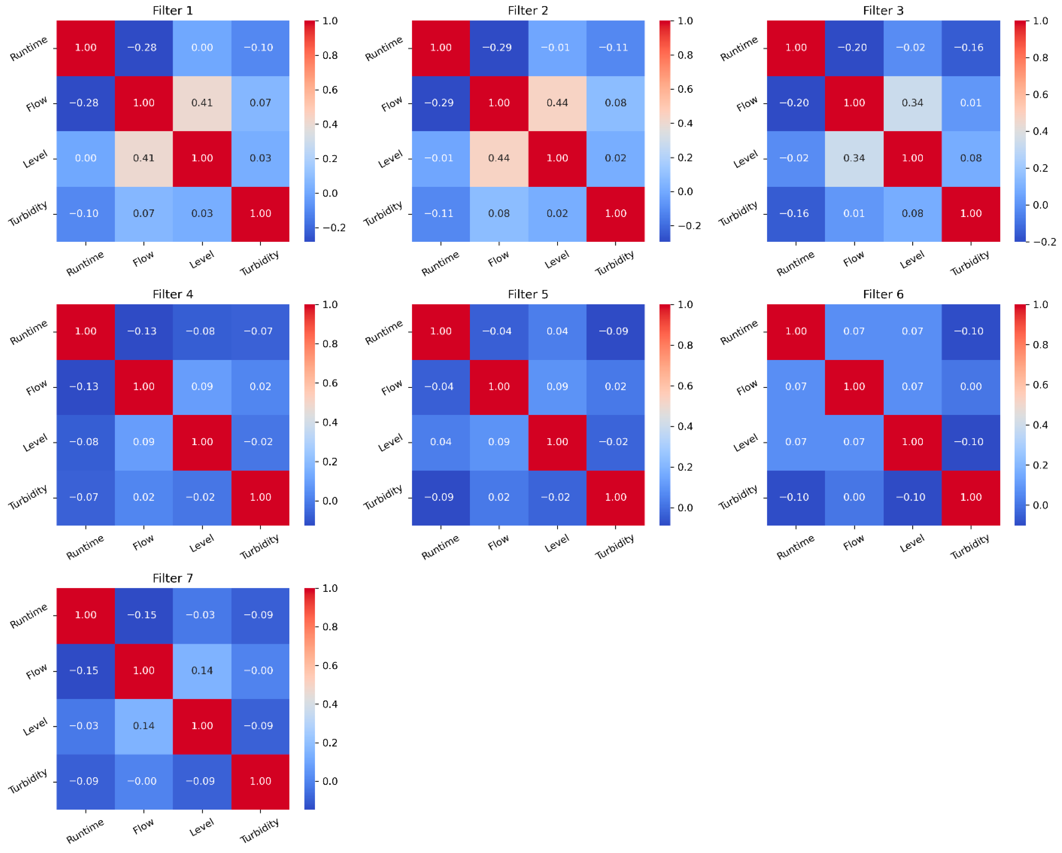
Figure 3 shows the Pearson correlation coefficients among the operational parameters and filtered water turbidity for Filters 1–7. A consistent positive correlation was observed between filter flow rate and bed level across all filters. This relationship was stronger between bed levels and filter flow rate was observed in Filters 1–3 compared to Filters 4–7, which may indicate flow maldistribution in these filters as a result of the influent lateral manifold [37].
Negative correlations were found between filter runtime and the filtered water turbidity, as well as flow rate and bed level for all the filters. Additionally, filters with stronger correlation between flow rate and runtime also tend to exhibit stronger correlations between runtime and bed level, suggesting interdependent operational behaviour.
Regarding filtered water turbidity, Filters 1–3 showed positive correlation with both flow rate and bed level. In contrast, Filters 4–7 exhibited a negative correlation between these parameters. Overall, there was a negative correlation between flow rate and filtered water across all filters. Notably, the magnitude of the correlation between flow rate and filtered water turbidity in Filters 4–7 is comparable to that between runtime and bed level observed in Filters 1–3.
Effect of Filters on Turbidity
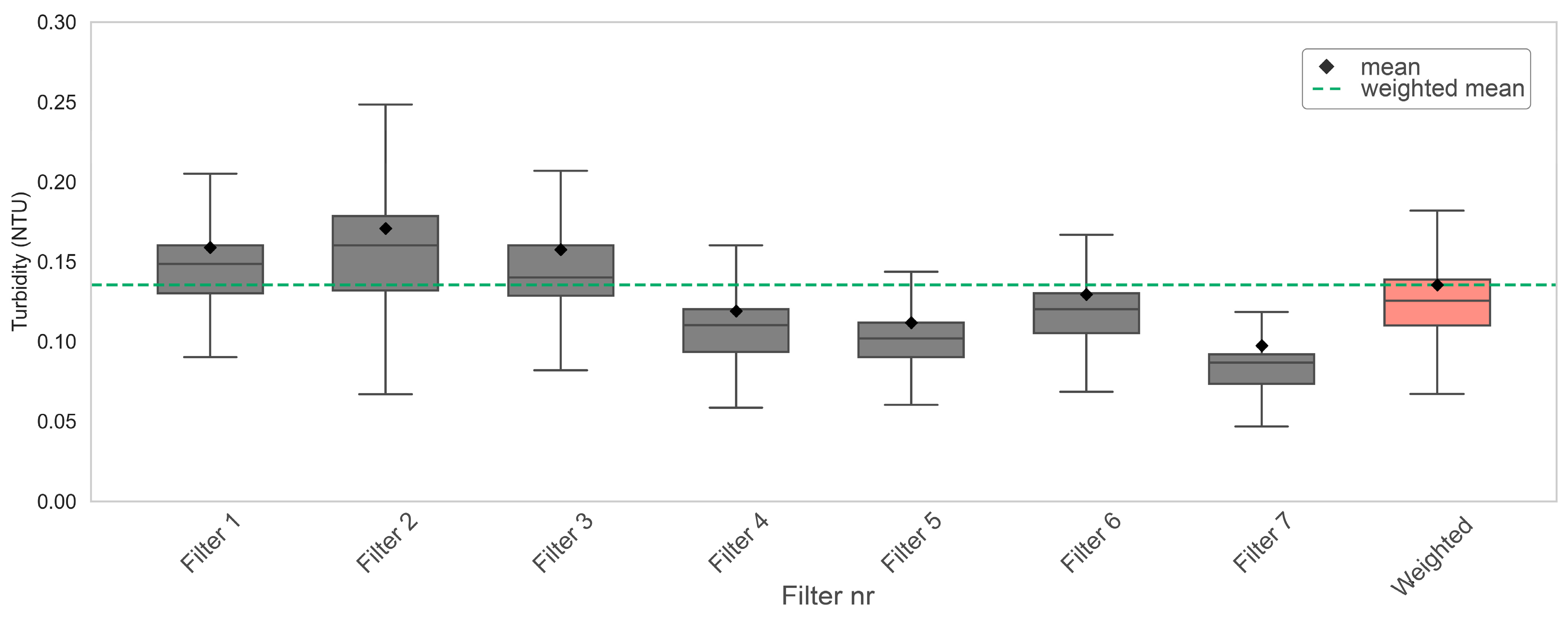
The individual filter turbidity is summarised in Figure 4 below and compared with the combined filtered water turbidity expressed as flow-weighted turbidity from Equation (1). The weighted filtered water turbidity ranged from 0.07 to 0.18, remaining well below the United States Environmental Agency (USEPA) provisions for combined filtered water [8,38]. Notably, Filters 1–3 exhibited mean filtered water turbidity slightly above the weighted average, whereas Filters 4–7 demonstrated lower individual turbidity values relative to the combined filtered water turbidity. Among all the units, Filter 7 consistently produced the lowest turbidity values, indicating the most effective performance over the study period. Figure 4 below presents a box plot showing the distribution of the turbidity in the filtered water.
This indicates that, at any point, the turbidity of the combined filtered water is reduced by the contributions of the other filters, which maintain a low turbidity, referred to here as the weighted turbidity.
Filter Flow Rate and Turbidity
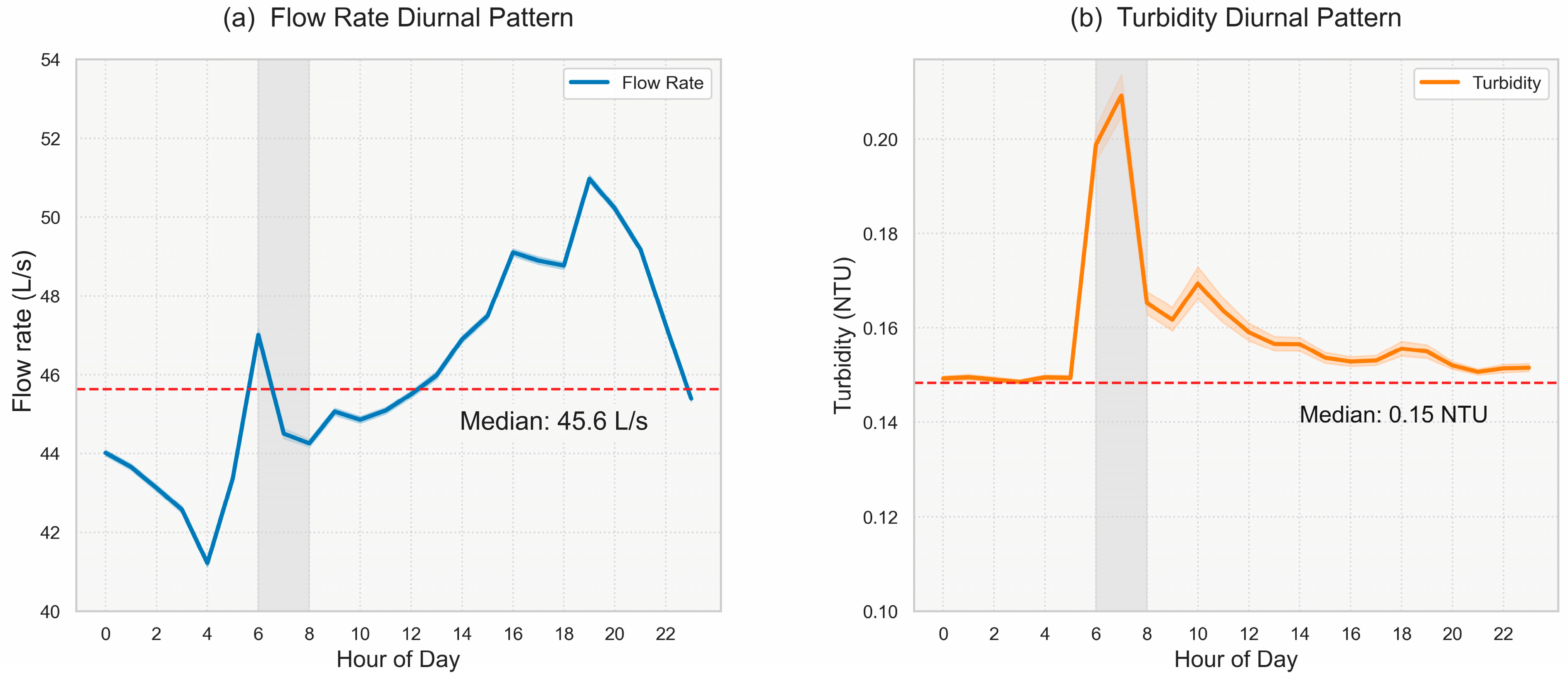
The patterns of the diurnal flow rate (a) and filtered water turbidity (b) are illustrated for Filter 1 in Figure 5 below. Typically, the flow rate at midnight is below the median line (45.6 L/s), along the decline from the evening maximum flow (~51 L/s) until it dips to its lowest (~41 L/s) at 4:00. The morning flow momentarily peaks (~49 L/s) at 6:00 and declines till 8:00. The flow rate increases steadily and is stabilised between 16:00 and 18:00 before reaching the maximum flow rate at 19:00.
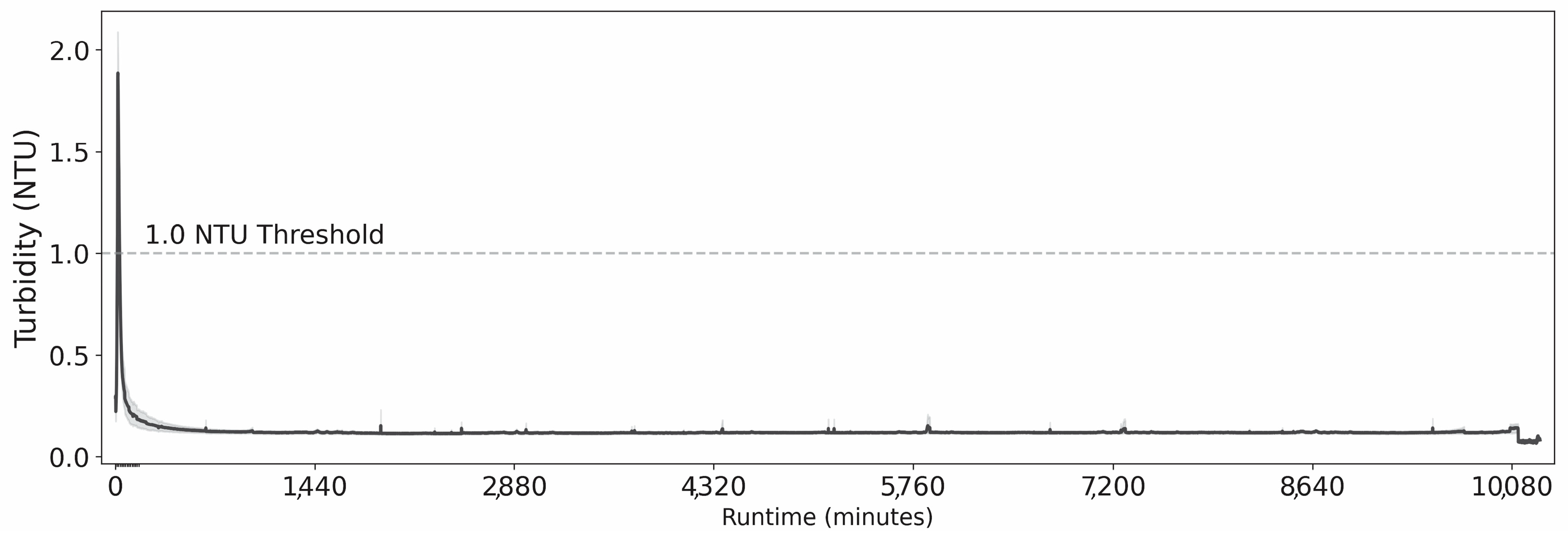
In Figure 5b, the filtered water turbidity curve starts at midnight slightly above the median (~0.15 NTU), increasing sharply to the first peak (>0.20 NTU) between 6:00 and 7:00, followed by an abrupt decline (~0.16 NTU) and minimal fluctuations until the next backwashing day. This pattern remains consistent across all filters due to the weekly backwashing routine process at 6:00, causing the observed spike in filtered water turbidity. During backwashing, the filter bed is fluidised, and particles are temporarily dislodged [39], causing an increase in the filtered water turbidity at the beginning of the new filtration cycle. The subsequent turbidity reduction from 0.21 NTU to 0.16 NTU (above the conventional 0.10 NTU threshold [8]) indicates the filter’s recovery after backwashing. This is primarily due to a decrease in the overall pore volume of the bed, which increases particle capture by interception and the contribution of other particle capture mechanisms in filters [40,41]. Additionally, the shape of the media also influences particle capture; therefore, media sharpness and the condition of the filter media, as well as replenishment, can significantly affect turbidity removal [39,42]. The second peak in flow rate at 19:00, however, corresponds to very minimal fluctuations in turbidity, indicating that turbidity is indirectly impacted by flow rate. The shaded regions in the respective figures (left and right) highlight the period of the highest increase in both flow rates and filtered water turbidity. This occurrence is due to the filter’s backwashing routine; the full effect is captured in Figure 6 showing a typical seven-day runtime for Filter 1.

3.2. Model Performance Evaluation for Filtered Water Turbidity Prediction

Six machine learning algorithms were evaluated to assess the effect of operational parameters and filtered water turbidity for the seven filters. For this, the performance using R2, MAE and RMSE of the filters after the baseline (MLR, SVR, KNN) and the ensembles (XGBoost, RF and ET) algorithms. The results for the assessment are presented in Table 3a,b below.
Table 3a,b shows a comprehensive comparison baseline models (MLR, SVR, KNN) and ensemble models (XGBoost, RF, ET) for predicting turbidity across seven different filter datasets, using R2, MAE, and RMSE as performance metrics. Best performing models for each filter in bold.
The results from Table 3 shows that the ensemble models consistently outperform baseline models across all filters and evaluation criteria due to their robustness in non-linear datasets [14,29,31]. Among the ensemble methods, Extra Trees (ET) is distinguished with the highest R2 scores and the lowest MAE and RMSE values, indicating its superior predictive performance. For instance, for Filter 3, ET achieves R2 = 0.92, MAE = 0.016 and RMSE = 0.016, which is notably better than the best performing baseline model—KNN; R2 = 0.70, MAE = 0.025, and RMSE = 0.073.
The baseline models present a mixed performance. Both MLR and SVR consistently yield low R2 values (all ≤ 0.23), and higher MAE and RMSE, indicating poor model fit and limited suitability for this regression task. KNN performs moderately well, achieving its best results on Filter 6 (R2 = 0.82, MAE = 0.022, RMSE = 0.054) and Filter 7 (R2 = 0.81, MAE = 0.019, RMSE = 0.047), comparable to the ensemble model’s performance. This observation is consistent with established literature, which indicates that non-parametric methods, such as KNN, generally perform better in low-dimensional spaces, although they struggle with more features or noise [43].
The ensemble methods, particularly ET and RF showed robustness and reliable performance across all seven filters. RF and ET maintained R2 values consistently above 0.79, with ET achieving the highest R2 score in four out of seven filters. For example, ET achieves R2 = 0.91 and MAE = 0.016 on Filter 6, compared to KNN’s R2 = 0.82, and MAE = 0.022. XGBoost also performs well, although it scores lower than RF and ET on some filters, emphasising its effectiveness in modelling the data’s underlying complexity [29]. The ensemble models, particularly RF and ET, provide superior and more consistent predictive performance for complex, non-linear relationships within this dataset [29,30].
The results demonstrate that ET and RF ensemble models offer superior and more consistent predictive performance for filter turbidity modelling compared to baseline approaches. These findings underscore the value of ensemble learning in modelling complex environmental datasets and support their adoption for robust turbidity prediction in water treatment applications.
Table 4 presents the A-TOPSIS (an approach based on the Alternative Technique for Order Preference by Similarity to Ideal Solution) ranking results for all the machine learning algorithms evaluated. The A-TOPSIS ranking reflects the overall performance, with lower ranks indicating better performance.
The A-TOPSIS ranking in Table 4 confirms that the ensemble models, ET and RF are the best in ranking, first and second, respectively, with their total scores (ET =1.00, RF = 0.83). SVR and MLR are the lowest ranking, indicating poorer overall performance, while KNN ranks third, outperforming XGBoost in the regression task.
Table 5 presents an aggregate comparison of the key performance characteristics of the three best-performing models: KNN, Extra Trees (ET) and Random Forest (RF).
Extra Trees and Random Forest demonstrate high predictive accuracy, consistently outperforming KNN, which gives moderate accuracy on the datasets. By comparing the computational performance of the algorithms on the datasets, KNN was the fastest model to train (~13 s), making it ideal for real-time applications with limited computational resources. However, this speed comes at the expense of lower accuracy and stability, since KNNs are known to be lazy learners [27]. ET achieves a balance with moderate training time (~620 s) and prediction time (~1 s) while maintaining the highest accuracy. Although RF delivers high accuracy, it is the slowest to train (~2100–2500 s), which may be considered for large-scale or time-sensitive applications. ET models, besides their accuracy, are faster because the algorithm is based on random splits, in contrast with RF models which find the optimal split by looking at all possible nodes [30].

3.3. Model Interpretation and Explainability

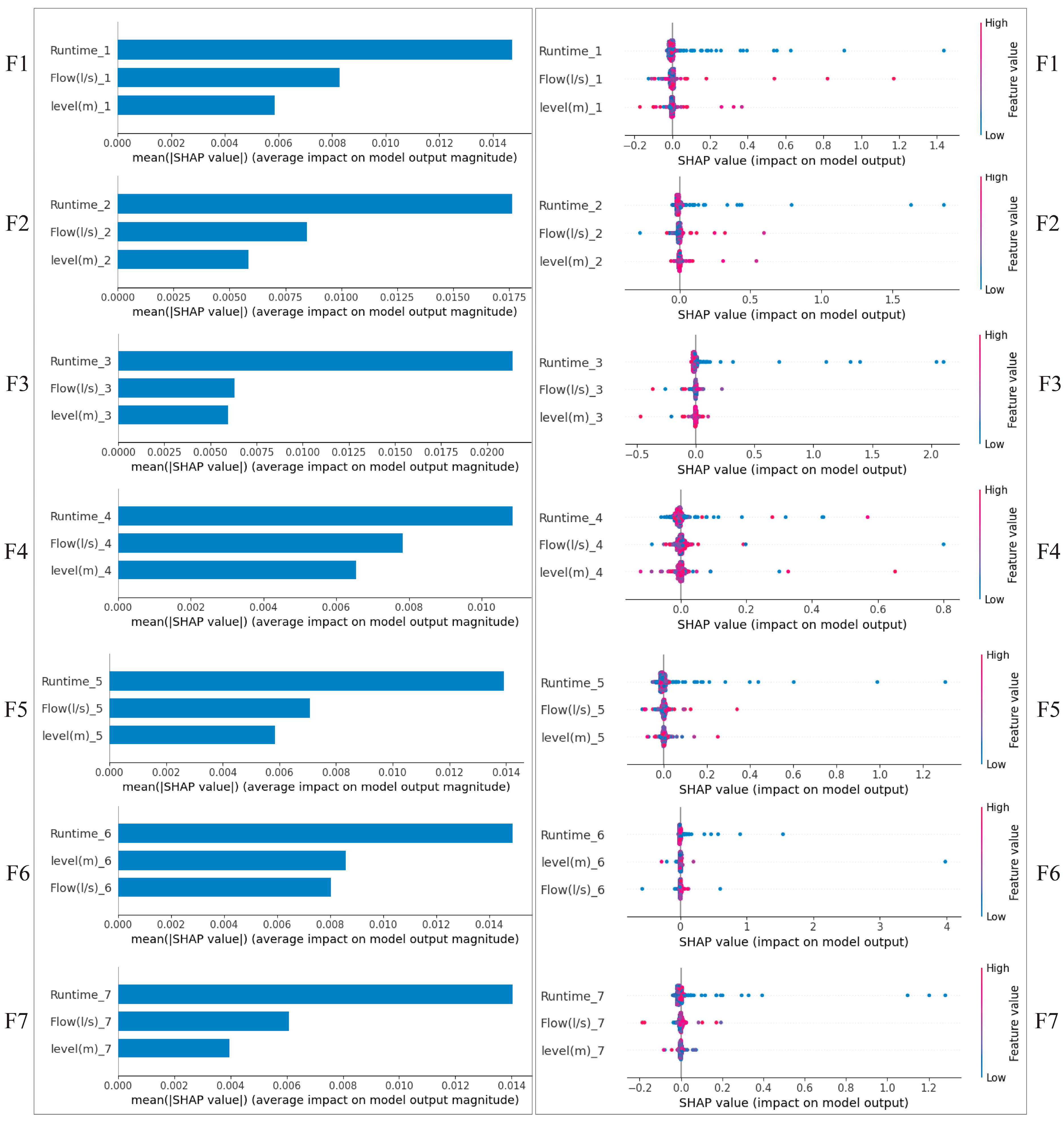
The TreeSHAP analysis discussed here only pertains to the ET models for the filters, as they demonstrated the best performance across all three metrics used to evaluate the models’ performance. Figure 7 below shows the global interpretations based on the average impact of the features on the model’s output. The left column bar plots, representing feature importance, display the mean absolute SHAP value for each feature in the ET models’ output for turbidity prediction, ranked by their importance. The right column scatter plots (summary plot) illustrate the individual predictions. The colour of the dots indicates the feature value, ranging from low (blue) to high (red) [44]. Positive SHAP values indicate a positive effect on the predicted variable and vice versa. Long tails for a feature suggest that a specific feature significantly impacts the model output [45].
From the bar plots, the generalised parameter trend is runtime > flow rate > bed level for all the ET filter models, except for Filter 6, where the bed levels are second to the filter runtime in feature importance. However, each ET model exhibits slight variations in the magnitude of their respective SHAP values and the corresponding impact, as demonstrated in the scatter plots. The effects of the features on the filters are discussed below.
The significance of feature importance fluctuates depending on the filter’s position, from 1 to 7. The most apparent differences among the three features were observed in Filter 3 (the highest R2 = 0.92). The summary plot in the right column illustrates that (i) lower runtimes positively influence the filtered water turbidity values; (ii) high flow rates also increase the filtered water turbidity, although only to half the degree of lower runtimes; and (iii) the bed water levels affect the filter’s performance in either direction, potentially increasing or decreasing the filtered water turbidity. On the contrary, the ET model for filter 4 is the worst-performing filter (R2 = 0.80) with average SHAP impact values of 0.010, approximately half that of Filter 3 (0.020) and 0.004 less than the other filters in the gallery, thus showing the weakest contribution to the filter. At the same time, the Flow and level parameters for the Filter 4 depict outlier situations as shown in the corresponding scatter plot [35].
Generally, increasing the runtime of the filters reduced the turbidity values and vice versa. Higher flow rates in Filter 6 have increased the predicted turbidity values. The bed level of Filter 3 has a negligible effect on the turbidity prediction. This implies a highly stable bed level throughout most filtration cycles. Therefore, while runtime is the dominant factor for effluent turbidity in Filter 3, increasing the flow rate impacts this trend, while the influence of bed level is negligible. In contrast with the other six filters, Filter 3 exhibits uniqueness in the trend of flow rates. The summary plot shows that the low flow rates in Filter 3 are as critical as the filter runtime in predicting turbidity.
The feature importance for all seven ET models of the filters indicates that the runtime feature is the most influential parameter, contributing to low filtered water turbidity in the mono-media filters.
For a local explanation of the factors, the predicted value, denoted in the force plot as f(x), is the contribution of the individual factors as arrows to the base value (expected output) of the entire dataset. The force plots for filters 1 to 7 (F1–F7) are shown in Figure 8 below. The force plots for the ET models regarding filters of the input features (runtime, flow rate, bed level) explain the predicted filtered water turbidity at a local level.
The runtime has a significant influence on the final prediction and is least affected by the bed level in the filter. For instance, using Filter 3 again for the explanation, the average prediction for the filtered water turbidity has a baseline ≈ 0.12 NTU, the runtime feature forces the predictions to the left by 0.01 NTU, and the filtered water flow rate further lowers the prediction in the same direction to 0.10 NTU by approximately similar units. The bed level makes a small push to the right to give the final prediction, and f(x) is 0.10 NTU.
By comparing the forced plots, we observe certain uniqueness in all seven filters. Filters 1, 2, and 3, have predicted filtered water turbidity values slightly higher than 0.10 NTU, whereas Filters 4, 5, 6 and 7 have predicted values ≤ 0.01 NTU.
At lower flow rates, the SHAP values for runtime are high, indicating that the filtration rate is crucial for the direct filters. An increased filtration rate may hinder effective particle removal, resulting in higher predicted filtered water turbidity [46]. As the flow rate increases, the SHAP values for runtime decrease, suggesting that the impact of runtime on turbidity prediction lessens at higher flow rates. This could be attributed to the fact that, at higher flow rates, particles are not effectively captured by the media [41]. This phenomenon relates to the properties of the filter media, such as diameter or material, which remain unaddressed in the machine learning models. Elevated turbidity in filtered water increases the risk of virus shielding and ineffective removal in the disinfection stage with UV light [47]. The elevated turbidity after backwashing can be improved by operating the filters based on predicted turbidity levels.

3.4. Implication of Predicted Filter Performance on Operation Routines

The WTP’s filtration operations encompass essential routines, such as backwashing and planned maintenance. The diurnal pattern of the Ålesund DWTP indicates that the plant has higher production during the evening compared to the mornings. This pattern occurs because the flow rate is reduced during backwashing routines, which involve isolating one of the seven filters. Consequently, there is a temporary decrease in the flow rate, which impacts the filtered water turbidity from the newly backwashed filter due to the disturbance during the backwashing period, as backwashing does not eliminate trapped particles completely. To address increased turbidity after backwashing, the start of the backwash filter is delayed for a few minutes before initiating the next filtration cycle. Although the SCADA data indicate that the system’s operation has experienced some flow reduction compared to the diurnal flow pattern, the corresponding flow data show that the flow is not significantly diminished. Furthermore, the SHAP interpretation for the best models in the case study indicates that the operational runtime for the filters can be extended by over seven days under the current operation of the plant.
Theoretically, the Length-to-Depth (l/d) ratio for this filter assembly is significantly lower than that of most rapid sand filters described in the literature. This emphasises the filters’ main purpose: pH correction, while enabling us to increase the l/d ratio. Reducing the effective diameter of the current filter media should be prioritised to enhance particle capture. Furthermore, the ultimate benefits would involve maintaining the upstream raw water turbidity < 5 NTU, as recommended for direct filtration setups. Nevertheless, the WTP’s downstream interventions, such as mixing the effluent from the seven filters and UV, are sufficient to meet today’s demands.
In applications, this study is applicable for developing soft sensors for each filter in DWTPs as either the main or a backup [16]. These soft sensors can be built as a stand-alone and updatable online platform to leverage data from the DWTP SCADA system. This online platform will provide early warnings and recommended actions to plant operators on the impact of specific operational conditions on filtered water turbidity levels.

4. Conclusions

The study employs three baseline and three ensemble machine learning models to investigate the prediction of filtered water turbidity in mono-bed filters at a drinking water treatment plant. The models were built using bed level, flow rate, and filter runtime as the primary parameters affecting the filtered water turbidity for a seven-unit filter bed. The filters generally behave similarly to the ripening stages of rapid media filters, typically expanding following backwashing. This resulted in increased turbidity for the unit filters immediately after the backwashing routine. The results from the Extra Trees (ET) ensembles achieved higher R2 values for all the filters (0.92) and the lowest RMSE (0.016 NTU), demonstrating their capacity to model complex relationships, although with slower computation times, compared to XGBoost models. The best-performing baseline model was KNN (R2 = 0.82 and RMSE = 0.054), ranking third after ET and RF models by the A-TOPSIS method. The SHAP feature analysis using the ET models highlighted significant operational parameters influencing filtered water turbidity, including filter runtime and filtered flow rate.
The predictive model developed in this study can help optimise mono-bed filter operations by providing early warnings of high turbidity levels. For instance, integrating AI in digital monitoring systems could enhance decision-making, reduce operational costs, and improve water treatment efficiency. It also fosters innovation in the management and optimisation of drinking water systems.
The approach presented offers a practical trade-off between accuracy and data availability in operational environments where long-term data collection may not be feasible. Since the models are trained on four months of operational data, their generalisability over a more extended period may be limited. However, they remain useful for seasonal use, provided they are regularly updated. Moreover, the study’s assumptions simplify the filtration process to the flow rate of the filtered water, bed level, and runtime of the filters, which may overlook critical physical complexities of filter dynamics. These include the length-to-depth ratio of the filters, flow regime within the filters, influent manifold correction factors, filter media roughness factors, and raw water quality. These complexities can be addressed by deploying hybrid models that incorporate fundamental filtration physics. For instance, the Tufenkji-Elimelech equation can be used to model particle capture and transport [41], and the Kozeny-Carman equation can account for operational headloss, bed level and filter characteristics. By using the outputs of these equations as augmented features in the model, the predictive performance of the data-driven methods can be substantially enhanced. Future studies will be evaluated using online SCADA data in real-time operations to assess their robustness and scalability while accounting for the physics of filtration.

Author Contributions

J.K.-K.: Conceptualisation, Methodology, Software, Writing—review and editing. H.M.T.: Methodology, Software, Writing—review and editing. R.S.: Supervision, Resources, Conceptualisation, Methodology, Writing—review and editing. All authors have read and agreed to the published version of the manuscript.

Funding

This research was funded by Regionale forskningsfond (RFF) Møre og Romsdal, DigiWater Project (Project No.: 341424).

Data Availability Statement

The data is owned by the Ålesund Drinking Water Treatment Plant. Available on request.

Acknowledgments

We acknowledge Tore Flisnes and Bjørn Skulstad of Ålesund Kommune’s VA department for providing SCADA data and excursion trips to the Ålesund Water Treatment Plant.

Conflicts of Interest

The authors declare no conflicts of interest.

Abbreviations

The following abbreviations are used in this manuscript:
A-TOPSISAlternative Technique for Order of Preference by Similarity to Ideal Solution
DWTPDrinking Water Treatment Plants
ETExtra Trees
k-NNK-Nearest Neighbour
MAEMean Absolute Error
MLMachine Learning
MLRMultiple linear regression
NTUNephelometric Turbidity Units
R2R-squared
RFRandom Forest
RMSERoot Mean Square Error
SCADASupervisory Control and Data Acquisition
SHAPSHapley Additive exPlanations
SVRSupport Vector Regression
USEPAThe U.S. Environmental Protection Agency (EPA)
xAIexplainable AI
XGBoostExtreme Gradient Boosting

References

  1. Thorne, O.; Fenner, R.A. The impact of climate change on reservoir water quality and water treatment plant operations: A UK case study. Water Environ. J. 2011, 25, 74–87. [Google Scholar] [CrossRef]
  2. Cornwell, D.A.; MaCphee, M.J.; Brown, R.A.; Via, S.H. Demonstrating Cryptosporidium Removal using spore monitoring at lime-softening plants. J. Am. Water Work. Assoc. 2003, 95, 124–133. [Google Scholar] [CrossRef]
  3. Elimelech, M.; O’Melia, C.R. Kinetics of deposition of colloidal particles in porous media. Environ. Sci. Technol. 1990, 24, 1528–1536. [Google Scholar] [CrossRef]
  4. Amirtharajah, A. Some Theoretical and Conceptual Views of Filtration. J. Am. Water Work. Assoc. 1988, 80, 36–46. [Google Scholar] [CrossRef]
  5. Gregory, J.; Nelson, D.W. Monitoring of aggregates in flowing suspensions. Colloids Surf. 1986, 18, 175–188. [Google Scholar] [CrossRef]
  6. Hendricks, D.W.; Clunie William, F.; Sturbaum Gregory, D.; Klein Donald, A.; Champlin Tory, L.; Kugrens, P.; Hirsch, J.; McCourt, B.; Nordby George, R.; Sobsey Mark, D.; et al. Filtration Removals of Microorganisms and Particles. J. Environ. Eng. 2005, 131, 1621–1632. [Google Scholar] [CrossRef]
  7. Kawamura, S. Design and operation of high-rate filters. J. Am. Water Work. Assoc. 1999, 91, 77–90. [Google Scholar] [CrossRef]
  8. USEPA. Guidance Manual for Compliance with the Surface Water Treatment Rules: Turbidity Provisions; Office of Water: Washington, DC, USA, 2020.
  9. Hsieh, J.L.; Nguyen, T.Q.; Matte, T.; Ito, K. Drinking Water Turbidity and Emergency Department Visits for Gastrointestinal Illness in New York City, 2002–2009. PLoS ONE 2015, 10, e0125071. [Google Scholar] [CrossRef]
  10. Benjamin, M.M.; Lawler, D.F. Water Quality Engineering: Physical/Chemical Treatment Processes; Wiley: Hoboken, NJ, USA, 2013. [Google Scholar]
  11. Crittenden, J.C.; Trussell, R.R.; Hand, D.W.; Howe, K.J.; Tchobanoglous, G. Stantec’s Water Treatment: Principles and Design; Wiley: Hoboken, NJ, USA, 2022. [Google Scholar]
  12. Griffiths, K.; Andrews, R. Application of artificial neural networks for filtration optimization. J. Environ. Eng. 2011, 137, 1040–1047. [Google Scholar] [CrossRef]
  13. Moradi, S.; Omar, A.; Zhou, Z.; Agostino, A.; Gandomkar, Z.; Bustamante, H.; Power, K.; Henderson, R.; Leslie, G. Forecasting and optimizing dual media filter performance via machine learning. Water Res. 2023, 235, 119874. [Google Scholar] [CrossRef]
  14. Wan, L.; Gong, K.; Zhang, G.; Yuan, X.; Li, C.; Deng, X. An efficient rolling bearing fault diagnosis method based on spark and improved random forest algorithm. IEEE Access 2021, 9, 37866–37882. [Google Scholar] [CrossRef]
  15. Gyparakis, S.; Trichakis, I.; Diamadopoulos, E. Using Artificial Neural Networks to Predict Operational Parameters of a Drinking Water Treatment Plant (DWTP). Water 2024, 16, 2863. [Google Scholar] [CrossRef]
  16. Juntunen, P.; Liukkonen, M.; Lehtola, M.J.; Hiltunen, Y. Dynamic soft sensors for detecting factors affecting turbidity in drinking water. J. Hydroinform. 2012, 15, 416–426. [Google Scholar] [CrossRef]
  17. Raman, G.S.S.; Klima, M.S. Application of Statistical and Machine Learning Techniques for Laboratory-Scale Pressure Filtration: Modeling and Analysis of Cake Moisture. Miner. Process. Extr. Metall. Rev. 2019, 40, 148–155. [Google Scholar] [CrossRef]
  18. Kale, S.J.; Khandekar, M.A.; Agashe, S.D. Prediction of Water Filter Bed Backwash Time for Water Treatment Plant using Machine Learning Algorithm. In Proceedings of the 2021 IEEE 6th International Conference on Computing, Communication and Automation (ICCCA), Arad, Romania, 17–19 December 2021; pp. 113–116. [Google Scholar]
  19. SEKLIMA, Norwegian Centre for Climate Services. Observations and Weather Statistics. Available online: https://seklima.met.no (accessed on 22 April 2025).
  20. Vann-Net, Map with Waterbodies. Available online: https://vann-nett.no/waterbodies/101-1982-L (accessed on 12 April 2025).
  21. Mohammed, H.; Longva, A.; Seidu, R. Impact of Climate Forecasts on the Microbial Quality of a Drinking Water Source in Norway Using Hydrodynamic Modeling. Water 2019, 11, 527. [Google Scholar] [CrossRef]
  22. Elçi, Ş. Effects of thermal stratification and mixing on reservoir water quality. Limnology 2008, 9, 135–142. [Google Scholar] [CrossRef]
  23. Murray, D.; Stankovic, L.; Stankovic, V. An electrical load measurements dataset of United Kingdom households from a two-year longitudinal study. Sci. Data 2017, 4, 160122. [Google Scholar] [CrossRef]
  24. Su, X.; Yan, X.; Tsai, C.-L. Linear regression. WIREs Comput. Stat. 2012, 4, 275–294. [Google Scholar] [CrossRef]
  25. Quan, Q.; Hao, Z.; Xifeng, H.; Jingchun, L. Research on water temperature prediction based on improved support vector regression. Neural Comput. Appl. 2022, 34, 8501–8510. [Google Scholar] [CrossRef]
  26. Cristianini, N.; Shawe-Taylor, J. Support Vector Machines and Other Kernel-Based Learning Methods; Cambridge University Press: Cambridge, UK, 2004. [Google Scholar]
  27. Györfi, L.; Kohler, M.; Krzyżak, A.; Walk, H. k-NN Estimates. A Distribution-Free Theory of Nonparametric Regression; Springer: New York, NY, USA, 2002; pp. 86–99. [Google Scholar]
  28. Biau, G.; Scornet, E. A random forest guided tour. Test 2016, 25, 197–227. [Google Scholar] [CrossRef]
  29. Geurts, P.; Ernst, D.; Wehenkel, L. Extremely randomized trees. Mach. Learn. 2006, 63, 3–42. [Google Scholar] [CrossRef]
  30. Majidi, S.H.; Hadayeghparast, S.; Karimipour, H. FDI attack detection using extra trees algorithm and deep learning algorithm-autoencoder in smart grid. Int. J. Crit. Infrastruct. Prot. 2022, 37, 100508. [Google Scholar] [CrossRef]
  31. Chen, T.; Guestrin, C. Xgboost: A scalable tree boosting system. In Proceedings of the 22nd ACM SIGKDD International Conference on Knowledge Discovery and Data Mining, New York, NY, USA, 13–17 August 2016; pp. 785–794. [Google Scholar]
  32. Krohling, R.A.; Pacheco, A.G.C. A-TOPSIS—An Approach Based on TOPSIS for Ranking Evolutionary Algorithms. Procedia Comput. Sci. 2015, 55, 308–317. [Google Scholar] [CrossRef]
  33. Vazquezl, M.Y.L.; Peñafiel, L.A.B.; Muñoz, S.X.S.; Martinez, M.A.Q. A Framework for Selecting Machine Learning Models Using TOPSIS; Springer International Publishing: Cham, Switzerland, 2021. [Google Scholar]
  34. Nguyen, L.V.; Tornyeviadzi, H.M.; Bui, D.T.; Seidu, R. Predicting Discharges in Sewer Pipes Using an Integrated Long Short-Term Memory and Entropy A-TOPSIS Modeling Framework. Water 2022, 14, 300. [Google Scholar] [CrossRef]
  35. Lundberg, S.M.; Lee, S.-I. A unified approach to interpreting model predictions. In Advances in Neural Information Processing Systems; MIT Press: Cambridge, MA, USA, 2017; Volume 30. [Google Scholar]
  36. Molnar, C. Interpretable Machine Learning: A Guide for Making Black Box Models Explainable, 3rd ed.; Leanpub: Victoria, BC, Canada, 2025. [Google Scholar]
  37. Wang, H.; Marshall, S.D.; Arayanarakool, R.; Balasubramaniam, L.; Jin, X.; Lee, P.S.; Chen, P.C. Optimization of a fluid distribution manifold: Mechanical design, numerical studies, fabrication, and experimental verification. Int. J. Fluid Mach. Syst. 2018, 11, 244–254. [Google Scholar] [CrossRef]
  38. Lovdata. The Norwegian Regulation on Drinking Water. Available online: https://lovdata.no/dokument/SF/forskrift/2016-12-22-1868 (accessed on 2 August 2025).
  39. Kramer, O.J.I.; van Schaik, C.; Dacomba-Torres, P.D.R.; de Moel, P.J.; Boek, E.S.; Baars, E.T.; Padding, J.T.; van der Hoek, J.P. Fluidisation characteristics of granular activated carbon in drinking water treatment applications. Adv. Powder Technol. 2021, 32, 3174–3188. [Google Scholar] [CrossRef]
  40. Kim, J.; Tobiason, J.E. Particles in Filter Effluent:  The Roles of Deposition and Detachment. Environ. Sci. Technol. 2004, 38, 6132–6138. [Google Scholar] [CrossRef] [PubMed]
  41. Tufenkji, N.; Elimelech, M. Correlation Equation for Predicting Single-Collector Efficiency in Physicochemical Filtration in Saturated Porous Media. Environ. Sci. Technol. 2004, 38, 529–536. [Google Scholar] [CrossRef]
  42. Akkoyunlu, A. Expansion of Granular Water Filters During Backwash. Environ. Eng. Sci. 2003, 20, 655–665. [Google Scholar] [CrossRef]
  43. Hastie, T.; Tibshirani, R.; Friedman, J. Model Assessment and Selection. In The Elements of Statistical Learning: Data Mining, Inference, and Prediction; Springer: New York, NY, USA, 2009; pp. 219–259. [Google Scholar] [CrossRef]
  44. Futagami, K.; Fukazawa, Y.; Kapoor, N.; Kito, T. Pairwise acquisition prediction with SHAP value interpretation. J. Financ. Data Sci. 2021, 7, 22–44. [Google Scholar] [CrossRef]
  45. Lundberg, S.M.; Erion, G.; Chen, H.; DeGrave, A.; Prutkin, J.M.; Nair, B.; Katz, R.; Himmelfarb, J.; Bansal, N.; Lee, S.-I. From local explanations to global understanding with explainable AI for trees. Nat. Mach. Intell. 2020, 2, 56–67. [Google Scholar] [CrossRef] [PubMed]
  46. Xiao, D.; Nan, J.; He, W.; Zhang, X.; Fan, Y.; Lin, X. Effects of inlet water flow and potential aggregate breakage on the change of turbid particle size distribution during coagulation-sedimentation-filtration (CSF): Pilot-scale experimental and CFD-aided studies. Chem. Eng. Res. Des. 2025, 216, 135–148. [Google Scholar] [CrossRef]
  47. Templeton, M.R.; Andrews, R.C.; Hofmann, R. Removal of particle-associated bacteriophages by dual-media filtration at different filter cycle stages and impacts on subsequent UV disinfection. Water Res. 2007, 41, 2393–2406. [Google Scholar] [CrossRef] [PubMed]
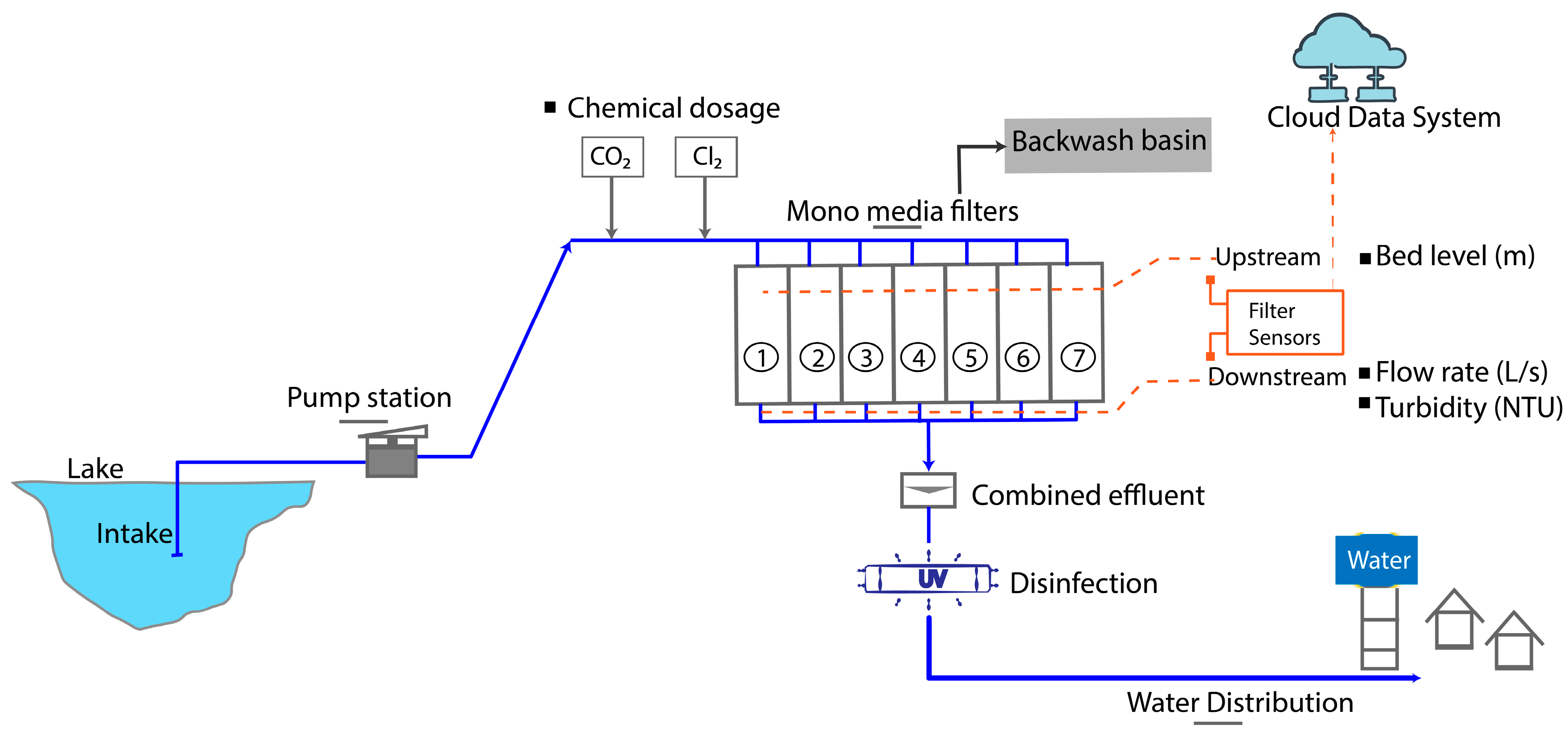
Figure 1. Overview of the Ålesund drinking water treatment plant. Mono-media filters nr. 1–7 correspond with numbers ①–⑦.
Water 17 02938 g001
Figure 2. Machine Learning Model Development Framework for DWTP filtered water turbidity.
Water 17 02938 g002
Figure 3. Relationship between filtered water turbidity and filter operation parameters.
Water 17 02938 g003
Figure 4. Box plot of filtered water turbidity for individual filters and combined filters (diamond markers show the mean turbidity of the respective filters). The green short dashes show the mean of flow-weighted turbidity.
Water 17 02938 g004
Figure 5. Diurnal patterns for (a) flow rate (L/s) and (b) filtered water turbidity for Filter 1.
Water 17 02938 g005
Figure 6. Typical filter turbidity profile for 7-day runtime.
Water 17 02938 g006
Figure 7. Global interpretation with SHAP plots: feature importance (left) and summary plot (right). The feature_(nr) corresponds to the feature of a particular filters 1–7.
Water 17 02938 g007
Figure 8. Local interpretation using SHAP explanation force plots for ET models for filters 1–7. Each subplot has a baseline value, which is forced to the left or right by the features to push the prediction value.
Water 17 02938 g008
Table 1. Hyperparameter search space for model prediction.
Model TypeHyperparameters
K-Nearest Neighbour‘n_neighbors’: [3, 5, 7, 9],
‘weights’: [‘uniform’, ‘distance’],
‘p’: [1, 2]
Random Forest‘n_estimators’: [50, 100, 200],
‘max_depth’: [None],
‘min_samples_split’: [2, 5],
‘min_samples_leaf’: [1, 2],
‘bootstrap’: [True, False]
Extra Trees‘n_estimators’: [50, 100, 200],
‘max_depth’: [None],
‘min_samples_split’: [2, 5],
‘min_samples_leaf’: [1, 2],
‘bootstrap’: [False]
Table 2. Summary data for Filters 1–7.
ParameterUnitMinMaxMeanStd.
Filtered Water Flow RateL/s0121.9746.439.65
Bed Levelm3.565.584.400.26
Filtered Water TurbidityNTU0.0110.00.130.12
Valve opening%0.00100.069.420.9
Filter Runtimemin110,28348062904
Table 3. (a,b) Performance comparison of baseline models and ensemble models.
(a) Baseline Models
R2MAERMSE
FilterMLRSVRKNNMLRSVRKNNMLRSVRKNN
Filter 10.0100.1820.610.0330.0460.0240.1120.1020.069
Filter 20.0130.2280.790.0390.0470.0250.1630.1440.081
Filter 30.0320.1630.700.0400.0530.0250.1420.1330.073
Filter 40.0040.1850.630.0350.0430.0280.1020.0920.061
Filter 50.0110.1410.560.0100.0360.0270.1090.1020.076
Filter 60.0170.4700.820.0340.0450.0220.1220.0890.054
Filter 70.0110.1960.810.0320.0450.0190.1010.0910.047
(b) Ensemble Models
R2MAERMSE
FilterXGBoostRFETXGBoostRFETXGBoostRFET
Filter 10.610.810.860.0250.0170.0160.0710.0480.016
Filter 20.650.850.900.0270.0180.0170.0980.0620.017
Filter 30.660.890.920.0250.0160.0160.0840.0480.016
Filter 40.350.790.800.0290.0190.0190.0820.0470.019
Filter 50.490.790.820.0290.0180.0170.0780.0520.017
Filter 60.740.890.910.0230.0160.0160.0630.0400.016
Filter 70.750.870.870.0210.0140.0140.0510.0370.014
Table 4. A-TOPSIS ranking of the algorithms.
AlgorithmRatioTotalRanking
ET0.29 ± 0.251.001
RF0.24 ± 0.230.832
KNN0.20 ± 0.160.643
XGBoost0.18 ± 0.140.534
SVR0.06 ± 0.110.105
MLR0.03 ± 0.110.016
Table 5. Overall performance of the top three models.
MetricExtra TreesRandom ForestKNN
AccuracyHighHighModerate
StabilityConsistentConsistentFilter-dependent
MAE~0.014–0.018~0.014–0.018~0.020–0.030
RMSELowest (~0.036–0.045)Low (~0.04–0.05)Higher (~0.07)
TrainingMedium (~620 s)Slow (~2100–2500 s)Fast (~13 s)
PredictionMedium (~1 s)Medium (~0.4 s)Fast
Disclaimer/Publisher’s Note: The statements, opinions and data contained in all publications are solely those of the individual author(s) and contributor(s) and not of MDPI and/or the editor(s). MDPI and/or the editor(s) disclaim responsibility for any injury to people or property resulting from any ideas, methods, instructions or products referred to in the content.