Abstract
The interaction between groundwater and surface water can be significant in lakes or irrigation channels, as well as in large dam reservoirs or along portions of them. To evaluate this interaction at a sampling location directly controlled by a large dam equipped with reversible pump-turbines, data from Rn-222 and physicochemical parameters at specific depths and times were obtained and studied using Principal Component Analysis and Hierarchical Clustering. Dimension 1 explains 45.3% of the total variability in the original data, which can be interpreted as the result of external factors related to seasonal variability (e.g., temperature, turbulent flow, and precipitation), while Dimension 2 explains up to 31.2% and can be interpreted as the variability related to groundwater inputs. Five hierarchical clusters based on these dimensions were considered and were related to the temporal variability observed in the water column throughout the year, as well as the depth relationships observed between successive surveys. A hypothesis-driven conceptual piston-like effect model is proposed for groundwater–surface water interactions, considering the identified relationships between variables, including higher Rn-222 concentrations in surface water after heavy rain. According to this simplified conceptual model, water infiltrates in a weathered granitic recharging area; during heavy rain, it is forced through the fracture systems of a lesser-weathered granite. Thus, an overall increase in pressure over the hydrological system forces the older radon-enriched water to discharge into the Mondego River. This work highlights the importance of exploratory techniques such as PCA and Hierarchical Clustering, in addition to underlying knowledge of the geological setting, for the proposal of simplified conceptual models that help in the management of important reservoirs. This work also demonstrates the utility of Rn-222 as a simple tracer of groundwater discharge into surface water.
1. Introduction
Water quality and management, as well as the affected ecosystems, are prioritized in European policies [1]. To optimize these processes, the interactions between different hydrosphere subsystems should be carefully considered and understood [2,3,4,5]. Different external factors impact groundwater and surface water to different extents [6,7,8,9,10]; however, the two systems interact and thus also impact each other [2]. Other physical factors, such as geology or geomorphology, spatially constrain the composition and movement of water [11,12,13,14,15]. The study of storm events can provide information on the movement of water into and through catchments, as well as on the geological structure underground [16,17,18,19]. General conceptual models include those describing the simple overland flow without groundwater contribution, the quick response of pipe flow, the throughflow in an unsaturated zone, and the pushing of older water via piston flow [16]. These simple, yet powerful conceptual models can indicate the velocity of water movement and the depth of the water source [16,17,18,19,20]. When combined with knowledge regarding the geological setting, these models enable the interpretation of important properties related to the flow path. Other, more complex models integrate mixing properties relating to different groundwater endmembers or mixing between groundwater and surface water, including exchanges in the hyporheic zone [21,22]. However, an increase in model complexity comes at the cost of an increase in data demand. Thus, simpler hydrogeological conceptual models of the flow paths that govern the interaction between groundwater and surface water are preferable as a first step in the development of conceptual models of underexplored or poorly studied hydrogeological systems [19].
Rn-222 (the most abundant naturally occurring isotope of the radioactive noble gas radon, which decays from Ra-226) has been used in multiple studies to effectively trace groundwater–surface water interactions (e.g., [23,24,25,26,27,28,29,30,31,32,33,34,35,36]). Here, Rn-222 is used to identify and characterize the discharge of groundwater into a section of surface water, influenced by a large dam equipped with reversible pump-turbines. Its variability with depth and with time, in conjunction with other physicochemical parameters [i.e., pH, electrical conductivity (EC), redox potential (ORP), and temperature (T)] in an artificial lake—the Aguieira Dam reservoir (central Portugal)—has been studied in [37]. The water column of this surface water undergoes periods of stratification and homogeneity due to natural factors and in response to the dam’s management. The complex interplay of natural and human factors can result in water quality problems [37]. The novelty of the database, covering an entire hydrological year and including samples at different depths of the water column in a section of surface water strongly influenced by anthropogenic management, raised awareness of the importance of monitoring surface waters and assessing Rn-222 endmembers for conceptual modeling. This, in turn, emphasized the importance of water flow paths, which are constrained by the hydrogeological and structural characteristics of the catchment [11,12]. Concerns about the vertical variability of natural lakes [38,39] and the assessment of groundwater endmembers [39,40] have been raised in the literature. Groundwater could account for 50–90% of the total uncertainty in quantitative models [38]. Recently, a novel method [36] was proposed for assessing the Rn-222 endmember independently of groundwater measurements. Nevertheless, studies often neglect to account for geology and structural geology variability [41], which is especially relevant in complex hydrogeological systems.
In this study, this subject is further analyzed with more robust exploratory techniques, including Principal Component Analysis (PCA) and Hierarchical Clustering (HC). The main goal is to understand the principal components affecting the temporal and depth-driven variability of the surface water and propose a valid, hypothesis-driven conceptual model of the contribution of groundwater to surface water, considering the interplay of variables in the water column throughout the year and their relationships with external pressures. The geological and structural settings are also closely examined, in order to emphasize their influence on the conceptual model’s formulation.
Multivariate analysis is widely performed in environmental sciences research, including, to some degree, in hydrogeological studies focused on groundwater (e.g., [42,43]) or surface water studies (e.g., [44,45,46]), as a data-driven methodological alternative to more common model-based approaches (e.g., [47,48]). Although with less frequency, these techniques have also been applied to study the interaction between groundwater and surface water at different scales (e.g., [49,50,51]). The authors of Ref. [52] emphasized the importance of geological knowledge for interpreting the results of dimensionality reduction techniques. Limited studies have incorporated radon gas into multivariate analysis with dimensionality reduction to study a hydrogeological system (e.g., [53]). To the best of the authors’ knowledge, this combination of variables and techniques has never been applied to study the groundwater–surface water interaction in a lake. Thus, the present study highlights the utility of Rn-222 as a tracer of groundwater discharges into surface waters, even in reservoirs with very large water volumes. Through a multivariate approach, this study highlights the value of information provided by Rn-222, accounting for its properties and its relationship with Ra-226, conditioned by geology; the methodology is also very cost-effective. These characteristics are very important for obtaining preliminary knowledge, translated into conceptual models, of areas and even scenarios such as the one discussed here—a river influenced by a large dam equipped with reversible pump-turbines—on which few studies have been published.
2. Setting of the Study Area
Sampling was carried out at a single location subject to the influence of the Aguieira Dam reservoir (Central Portugal) and at different water column depths, with significant differences in depth throughout the year (a maximum of 10 m and a minimum of 4 m, approximately). Aguieira Dam is a multi-arch dam with 89 m height and a 400 m crest, located in the Mondego River drainage basin (Central Portugal). It is equipped with three reversible pump-turbine groups. The reservoir has three main inputs: the upstream inflow, the groundwater, and the pumped water from downstream. The two main outputs are the turbined water and the discharged water. The water management of the Aguieira Dam affects the water level in the sampled location [N 40.40211°, E 7.98739° (WGS84)], about 20 km upstream (Figure 1; [37]).
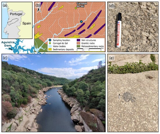
Figure 1.
Geographical and geological setting of the study: (a) geographical setting of the Mondego River basin; (b) simplified geological cartography of the studied region at a scale of 1:500,000; (c) outcropping granitic rocks (round-shaped blocks) in the riverbed at the sampling location; (d) detail view of coarse-grained porphyritic biotite-bearing granite with feldspathic phenocrysts; (e) granite with microgranular tonalite and metasedimentary xenoliths.
According to [54] and the Köppen–Geiger climate classification, the studied area is characterized by a temperate, dry, and hot summer (Csb) climate. Typically, the summer has high temperatures, intense sun, and very low precipitation. The winter is influenced by Atlantic fronts, which are responsible for most of the precipitation [55]. The Portuguese climate is changing towards a hotter and possibly drier climate [56]. In 2023, winter showed slightly positive anomalies in temperature and precipitation compared to the 1981–2010 average. Spring had significantly high temperatures and low precipitation, while summer experienced positive temperature anomalies and increased precipitation in June. Fall also had higher temperatures and significant rainfall [56].
At the sampled location, a coarse-grained porphyritic biotite-bearing granite with feldspathic phenocrysts (Figure 1) outcrops from the Batholith [Figure 1a]. Microgranular xenoliths of tonalite and enclaves of metasedimentary rocks were observed in the outcrops [Figure 1e]. The granite is classified as C2 following the classification proposed by [57]. Other authors who studied this same granite in the region have classified it as Tábua Granite [58] and G2 [59]. The region includes an intense network of faults, commonly filled with brecciated granite. The fault filling can range from a few centimeters to several meters [58,60,61].
The outcropping granitic rocks show very different weathering conditions. The Beirão plateau, where the Mondego River has incised its course, is characterized by a large region of very weathered granitic rocks. On the steep slopes of the river incision, less weathered granitic outcrops can be observed [Figure 1c]. According to the conjunctural land use cartography [62], the plateau is mainly occupied by agricultural lands and underbrush and herbaceous vegetation. Artificialized land is restricted to relatively small villages. The slopes are occupied by forest with large trees (mainly eucalyptus).
At present, the major principal stress (σ1) acting over the west of the Iberian Peninsula is NW-SE-oriented, whereas the minor principal stress (σ3) is NE-SW-oriented [63]. Lineaments in the studied area were identified and are presented in a rosette diagram in Figure 2. The predominant orientation of the lineaments identified in the region is N45–65° E (Figure 2), which is the general orientation of the Mondego River in the region. The orientations of other lineament systems were also identified; namely, E-W, N20° W, N50° W, and N70° W.
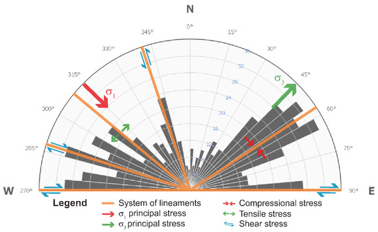
Figure 2.
Rosette diagram of the orientations of principal lineaments and interpreted stresses currently acting on them. Lineaments were identified via aerial photography and a Digital Elevation Model built with them (unpublished data). Principal stress tensors (σ1 and σ3) were retrieved from [64].
3. Materials and Methods
3.1. Data Availability
Available data are organized in time through nine vertical surveys (S1 to S9), from May 2022 to September 2023, with a time gap of 8 months from the first to the second survey. For each survey, the Rn-222 concentration (RC), pH, EC, ORP (except for S1), and T were obtained. The first survey (May of 2022) in [37] was excluded from the analysis because no data on ORP were available. More details of the surveys, including sampling dates, are provided in Table 1.

Table 1.
Survey details.
All the logistics involved in the seasonal sampling campaign, including in situ measurements of the physicochemical parameters, are described in [37]. Water samples were collected at various depths at the center of the river, using a specially designed sampler described and validated in [64], in which the protocol for the sampling of water and measurement of RC is fully detailed. The sampling procedure was as follows: The sampler was lowered from a bridge above the sampling location at incremental depth steps; each depth sample was taken into the air-tight samplerand brought back. First, 10 mL of the sample was taken for RC analysis and the following 500 mL for ORP measurement, and then the remaining parameters were analyzed. The RC sampling uncertainty was estimated to be 5% (k = 2), and the total measurement uncertainty was estimated to be 15% (k = 2) [64].
The RC surveys are shown in Figure 3. As stated in more detail in [37], a transition in the water column and characteristic Rn-222 signals can be observed. In periods of stratified water column (S1, S7, and S8), the epilimnion is depleted of radon gas due to degassing; the thermocline shows a higher RC, with an RC increment at the bottom. Stratification occurs with the water level at its highest before and during the beginning of the summer season, when there is no significant precipitation but the dam’s reservoir discharge is limited to accommodate water for the summer. In the winter season (S2 to S5), the water column is more homogeneous, although, after periods of heavy rain (S4 and S6), the RC is higher and it increases toward the top of the water column. After the summer season, with the water level at its lowest, stratification was not present, and the RC was high. The survey results for the remaining parameters are shown in Supplementary Material Figure S1.
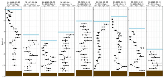
Figure 3.
Vertical surveys of Rn-222 concentrations in the surface water. Adapted from [37]. Surveys (S) are organized from S1 to S9 according to the date of sampling. Blue straight lines represent the water level.
3.2. Statistical Analysis
For statistical analysis, RC results below the limit of detection (LD) were substituted by 0.65×LD, in line with [65]. Statistical analysis was performed using the R Language [66] with the Stats [66], GGally [67], and Hmisc [68] packages.
3.2.1. Principal Component Analysis
Principal Component Analysis (PCA) is a mathematical method for reducing the dimensionality of multivariate data into principal components (PCs), which are orthogonal (uncorrelated) dimensions obtained from linear transformations of the original variables [69,70]. This technique was used as an exploratory technique to complement cluster analysis, whose main goal is not to directly reduce the dimensionality. The implementation of PCA relies on Singular Value Decomposition (SVD), a generalization of Eigendecomposition. Since PCA has been widespread for many years and used in many scientific fields, no details will be provided here. For additional details on PCA, please see [70,71,72,73].
The significance of PCs is not easily assessed, as no distribution assumptions are established [7]. Nevertheless, for the proposed interpretation of the first two PCs of the PCA, two tests were applied to evaluate the suitability of the data and the PCA method for the study’s purpose: (i) Bartlett’s test of Sphericity [74] to evaluate the null hypothesis of the correlation matrix being an identity matrix (a significant test result would imply that the null hypothesis is very unlikely, indicating relationships between the variables in our data); and (ii) the Kaiser–Meyer–Olkin (KMO) test [75] to evaluate the sampling adequacy based on global and partial correlations. Both tests were implemented through the psych R package (version 2.4.1) [76].
The dataset with the measured variables, i.e., RC, pH, EC, ORP, and T, of each survey was therefore analyzed using PCA, implemented through the R packages stats [66] and factoextra [77]. The data matrix was centered and scaled.
3.2.2. Hierarchical Clustering
Hierarchical Clustering, another multivariate technique, was mainly used in this study to identify possible clusters of samples. It was performed with the R implementation of the agnes (Agglomerative Nesting) algorithm [78] in the R-package cluster [79]. The distance used to measure dissimilarity was the sum of absolute differences, and Ward’s criterion [80] was used to minimize the within-cluster variance. The optimal number of clusters was evaluated through the average silhouette width [78], which measures the average distance between clusters. The aim of this method is to find the clustering structure that maximizes this distance, although the optimal number of clusters was selected based on the visual investigation of the total within-cluster sum of squares (scree test; [81]). The idea behind this method is to obtain compact clusters by minimizing the total intra-cluster variation, which requires the analyst to choose the best trade-off (“elbow”) between increasing the number of clusters and minimizing the total-within-cluster sum of squares.
4. Results
A significant Bartlett test result (p-value < 0.001) was obtained, indicating that the correlation matrix is significantly different from an identity matrix. The KMO test revealed a measure of sampling adequacy (MSA) above 0.5 for all the variables (RC MSA = 0.67; pH MSA = 0.57; EC MSA = 0.52; ORP MSA = 0.59; T MSA = 0.56) and an overall MSA of 0.56, which indicates that the data is suitable for the proposed PCA. A ratio of 22.2 samples (total of 111 samples) per variable (total of 5 variables) is also indicative of the sampling adequacy based on common rules of thumb [82]. The PCA results are expressed in Figure 4. PC 1 (45.3%) and PC 2 (31.2%) explain up to 76.5% of the total variability in the original data (Figure 4a; Table 2). Dimension 1 separates ORP from pH, temperature, and EC, and dimension 2 differentiates pH from RC, ORP, EC, and temperature (Figure 4b). As only RC contributes significantly to the third dimension (Table 2), PC3 was excluded from further analysis.
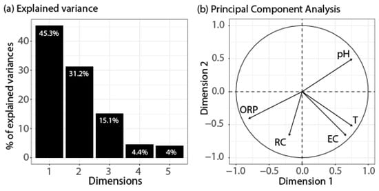
Figure 4.
Principal Component Analysis results for the Rn-222 concentration (RC), redox potential (ORP), electrical conductivity (EC), temperature (T), and pH. (a) Histogram of the percentage of the variance explained by the principal components (dimensions). (b) Variable loadings projected on the biplot of dimensions 1 and 2.
Table 2.
Principal Component Analysis results: Eigenvalues of the dimensions, the contribution of each variable to each dimension, and the percentage of the total variance explained by each dimension.
Clustering was performed based on the scaled data from the first two dimensions. To evaluate the optimal number of clusters, two measurements were computed: (i) the average silhouette width (Figure 5a) and (ii) the total within sum of squares (Figure 4b). The silhouette method showed a higher silhouette for two clusters, which would correspond to the fourth cluster in Figure 5c, comprising the shallower samples of S7. The silhouette drops but remains steady for a larger number of clusters. This indicates that, despite clusters being close to each other, clustering maintains a structured hierarchy. Therefore, the scree plot was visually interpreted (Figure 5a) to investigate the best trade-off between increasing the number of clusters and minimizing the intra-cluster variation. After five clusters, the decrease in total within sum of squares for one more cluster was considered to be minimal (less than 2% reduction in the total within sum of squares for one cluster). The resulting clusters are projected in Figure 5c. Dimension 1 is responsible for the clear differentiation of the fourth cluster, mainly composed of the shallower samples of S7 (Figure 5b). On the other hand, dimension 2 defines the second cluster, composed of the S2 and S3 data, with the third cluster aggregating the shallower samples of S8 and the deeper samples of S7, and the fifth cluster aggregating S9 data with the deepest data of S8.
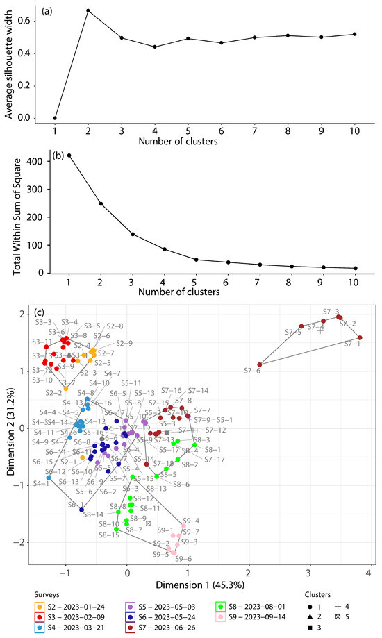
Figure 5.
Clustering analysis results of the depth-specific data of Rn-222 concentration (RC), redox potential (ORP), electrical conductivity (EC), temperature (T), and pH. (a) Average silhouette width. (b) Total within sum of squares as a function of the number of clusters. (c) Projected data on the biplot of dimensions 1 and 2, grouped by clusters defined and colored according to the sampling surveys. Samples are incrementally numbered according to the ith depth steps of the water column (e.g., S9-1 corresponds to the first sample, the most superficial, of survey S9; please refer to Figure S1 for the absolute depth of each sample).
5. Discussion
5.1. Groundwater Endmember
In most scenarios, Rn-222 concentrations are significantly higher in groundwater than in surface water, making it a good tracer of groundwater inputs. However, this is not always the case, and here, due to the large volume of water in the reservoir and the time-series analysis, special attention is given to this endmember; namely, to the relationship between groundwater and surface water concentrations and to the groundwater variability over time. Groundwater samples were collected at locations near the sampling site, covering the same period under study but on different dates. Time series of the Rn-222 concentrations for three sampling sites are presented in Figure 6 These are natural springs that freely discharge throughout the year. GW1 (µ = 711 ± 172) and GW2 (µ = 710 ± 78) are located a couple of kilometers away from the sampling location of surface water, at the top of the Beirão plateau, but GW3 (µ = 313 ± 184 Bq/L) is located just a couple of meters away, in a steep v-shaped valley. The minimum, median, and maximum values of the studied parameters, i.e., temperature, pH, EC, and RC, are expressed in Table 3 and compared to the same variables in the surface water under study.
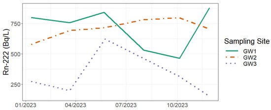
Figure 6.
Radon-222 concentrations of three groundwater samples taken near the surface water sampling site under study.
Table 3.
Descriptive statistics—median (minimum–maximum) values of temperature, pH, electrical conductivity (EC), Rn-222, spring discharge, and redox potential (ORP) for all the samples of surface water from the sampling location and the groundwaters.
Groundwater samples at the top of the Beirão plateau—the recharging area—show relatively low variability, especially GW2; this variability falls within the uncertainty range of the technique. This suggests that the Ra-226 content in the groundwater at the plateau is relatively stable and in equilibrium with that in the rocks. On the other hand, GW3 shows high variability (coefficient of variation of 59%). No correlations were found between RC at each groundwater sampling site and the precipitation or the maximum RC found in surface water.
RC in groundwater at the top of the plateau is 450 times higher than that in the studied surface water, and groundwater sampled at the slope of the valley has approximately 200 times higher RC. This indicates that RC is a good tracer of groundwater inputs into the surface water. The relatively high variability found at the valley suggests that other factors influence the groundwater flow, such as the path or the residence time.
5.2. Dimensionality Interpretation
Principal components (PCs) are linear transformations of the original variables. Therefore, there is no simple interpretation for them [68]. However, they often represent meaningful physical phenomena in natural sciences, particularly the first few components.
In this work, dimension 1, which accounts for 45.3% of the total variability in the data (Table 1), can be interpreted as the seasonal variability, mainly influenced by external factors such as temperature, turbulent flow, and precipitation. As external forces promote increases in temperature, pH, and EC, the ORP tends to decrease. The negative loading for RC in this dimension, though closer to zero, is a result of RC only being influenced by those pressures in the uppermost and shortest water layer—the epilimnion.
For example, with higher atmospheric temperature in the middle of the summer season, the water temperature increases, and the water level drops, which increases the concentration of dissolved solids [37]. A stratification of the water column is also present, which deteriorates water quality. The increased biological activity, changes in the water chemical composition, and nutrient availability all contribute to the increase in water pH. Conversely, ORP is the only variable that significantly decreases because of the lack of dissolved oxygen in the water due to the higher water temperature. Radon is only affected by the atmospheric temperature in the epilimnion; namely, decreasing due to degassing. During the rainy season, for example (see S2, S4, and S6 in Figure S1; [37]), when rain and associated turbulent flows increase and the atmospheric temperature is lower, the water temperature is colder and the pH has been shown to be lower. EC is also reduced due to the higher volume of flowing water. Conversely, the ORP is higher: this is explained by the water’s increased oxygenation, promoted by the turbulent flow, which increases the contact surface for gaseous exchange with atmospheric oxygen, and the incorporation of oxygen into raindrops and subsequently into the surface water. Radon was also found to increase after significant precipitation, especially in the epilimnion (see S4 and S6 in Figure S1). This is discussed further for the second dimension and thereafter.
Dimension 2, which accounts for 31.2% (Table 2), can be interpreted as the groundwater input variability. Groundwater discharge increases RC and EC in the surface water and decreases the water pH (Table 3). Temperature should also increase in the winter or decrease in the summer; however, in [37], there was no evidence of significant temperature changes in groundwater with depth. Most of the variance in the measured temperature was attributed to seasonal variation. Therefore, the loadings of temperature and ORP in dimension 2 are due to the higher relative contribution of groundwater during the dry season.
Dimension 3 only explains 15% of the total variance (Table 2). The corresponding eigenvalue below 1 and the fact that only RC shows a significant correlation with this dimension indicate that this dimension is not significant, and should not be considered in the proposed analysis. The variability found is possibly the result of other factors that could not be interpreted in the conceptual model.
5.3. Temporal Variation in the Water Column
Clusters projected on the biplot of dimensions 1 and 2 (Figure 5b) can then be interpreted as resulting from variability with time and depth, which is mostly influenced by external factors and the groundwater input. Cluster 2, composed of surveys in January and February of 2023 (S2 and S3—Figure S1), includes samples affected by low temperatures, high turbulence, and fast flow, as well as smaller inputs of groundwater. This cluster shows no linearity between dimensions (Figure 5b) as a reflection of the homogeneity in the vertical surveys (Figure S1; [37]). Cluster 1 (Figure 5b), composed of surveys in March and May of 2023 (S4 to S6—Figure S1), is affected by slightly higher temperature, lower turbulent flow, and increased groundwater contribution, which is also related to precipitation [37]. In this cluster, linearity is observed in S4, with the first two samples (S4-1 and S4-2; Figure 5b) differentiated from those from the rest of the survey. The first three samples of S6 (S6-1 to S6-3; Figure 5b) are also differentiated from the rest of S6. These samples were in fact defined as the epilimnion in the corresponding surveys and were considered a signal of groundwater input [37]. The other three clusters (3, 4, and 5; Figure 5b) represent a transition in the water column. Cluster 4 (the most differentiated) includes the shallower samples of survey 7 (the most complete stratification of the water column considered for PCA; Figure 7; Figure S1; [37]). The samples show no trace of groundwater input (positive PC2; Figure 5b), which could also be influenced by Rn-222 degassing. For the study of water quality, it is important to note that this cluster is not coincident with thermal stratification (at a normalized depth of ~3.25 m; Figure 7), but instead with the stabilization of all the other variables (at a normalized depth of ~4.25 m; Figure 7). Cluster 3 incorporates the other samples of S7, with RC and EC as signals of groundwater input and lower temperature, and thus is not as influenced by atmospheric temperature and solar radiation. This cluster also includes samples from the top of S8, which are at an equivalent normalized depth of the first samples of S7 in this same cluster (e.g., S8-2, S8-3, S8-4, …, which are at the same depth of S7-7, S7-8, S7-9, …; Figure S1; [37]). Cluster 5 is characterized as the most affected by summer pressures and with the highest relative groundwater contribution. The time continuity (diagonal link of S8 and S9; Figure 5b) of the time-varying water column can also be visualized for this cluster, as was also possible in cluster 3 (diagonal link of S7 to S8; Figure 5b).
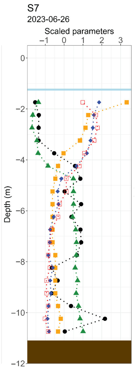
Figure 7.
Vertical survey S7 (June of 2023) of Rn-222 concentration (black filled circles), pH (blue filled rhombus), redox potential (green filled triangles), electrical conductivity (yellow filled squares), and temperature (red contoured squares) in depth. Values are scaled to show the relations between patterns. For original values, please refer to [37]. Blue straight lines represent the water level.
5.4. Hypothesis-Driven Piston Effect Conceptual Model for Groundwater–Surface Water Interaction
Considering the evidence of temporal variation in RC in the vertical surveys discussed in [37], as summarized through the PCA, and the geological setting of the studied area, a piston-like model is proposed for the groundwater–surface water interaction (Figure 8). The piston effect model has been applied many times over the years, including in different geological settings [8]. The water movement is modeled as a compact and delimited body, like a piston, that flows with very well-defined movement, thus transmitting its pressure through the water itself, pushing the older water and causing its discharge. Although this process can occur in different types of physical media, faults and joints represent well-defined paths of increased permeability relative to the almost impermeable granitic rocks, which constrain the water body such that it flows like a fast-moving piston. Although there is little literature that describes RC in these settings, the increase in RC after precipitation has previously been associated with the piston effect in detrital aquifers [26] and in karst settings, typically characterized by the presence of natural conduits carved by the water [83].
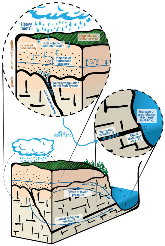
Figure 8.
Preliminary simplified hypothesis-driven conceptual piston-like model of water movement, especially important after storm events. The single-fault model is a visual simplification of a network of complex fault systems, with different strikes.
Precipitation itself is depleted of RC since RC in the atmosphere is relatively low [84,85]. Increased overland flow is also depleted of RC as the water does not infiltrate into the soil and rocks to dilute higher RC. At a large reservoir such as the Aguieira, which is not expected to have a large contribution of groundwater, significant precipitation over a large area would contribute directly to the dilution of RC and indirectly to a larger volume of runoff depleted of Rn-222, which would also contribute to its dilution.
An increment in RC is an indicator of a higher groundwater contribution, but a decrease in RC is not necessarily indicative of a diminished groundwater contribution [37,38]. During intense stratification of the water column, the vertical mixing is negligible, and radon degassing only occurs at the epilimnion [32,37]. Therefore, the maximum RC, or the local maximum in the stratified water column, is indicative of the groundwater input to the thermocline and hypolimnion. Then, the significant correlation found between maximum RC values, indicating groundwater inputs, and precipitation (RSpearmn = 0.77) is not easily explained. It was also verified that after heavy rains, the maximum RC was at the top of the surface water (S4 and S6—Figure S1), corresponding to the epilimnion [37], where degassing typically would occur, especially in highly turbulent water. Simple throughflow in the subsurface unsaturated zone is fast enough to explain the correlation between RC and the precipitation. However, in the studied area, the granitic outcrop is relatively unweathered, which does not explain the increased permeability that would enable throughflow through an unsaturated zone. Two reasonable hypotheses for the flow through the faults are considered: (i) after precipitation, water in the recharging area with higher RC and in equilibrium with the source rock is directed to the fault system and moves with high velocity over a shorter flow path, like a piston moving in a channel; or (ii) the increased hydrostatic pressure is transmitted through the faults and pushes deeper and “older” water, which has had time to equilibrate with the Ra-source rock and become enriched with its progeny—namely, Rn-222 gas—which is pushed in a piston-like process, triggered by the precipitation. Sample GW3’s variability and its lack of correlation with precipitation and maximum RC in the surface water suggest that water flowing along these shorter, NW-SE-oriented paths may not be responsible for the RC inputs, thus not supporting hypothesis (i); instead, in the proposed model, they could still act as a transmitter of pressure and push, to the surface, the water flowing in a deeper and more evolved fault system like the NE-SW-oriented one, where the river incises, as proposed in (ii).
As mentioned above (Section 2), the Beirão plateau is a significant recharging area due to the presence of weathered granitic rocks. This superficial weathered layer has significantly increased natural permeability, promoting water infiltration. This superficial layer gradually changes in depth to a less weathered granite, as observed in outcrops in the river’s margins, with significantly lower permeability, where faults and joints are the only main pathways for groundwater flow. After heavy rain, the infiltration of the rainwater into the unsaturated zone increases near the recharging area. The hydrostatic pressure over the aquifer itself and over the faults and joints increases. In the transition zone from the weathered to unweathered granite, water strangulation occurs in the faults and joints, and consequently, the velocity increases. The fractures act as a piston that transmits the pressure and increases the velocity through the water. The older water enriched in Rn-222 from greater depths could then be forced to the output with higher velocity, increasing the discharge flow to the surface water.
Under the present stress field (Figure 2; [63]), the N20° W, N70° W, and E-W orientations, which are under shear stresses, are preferable water paths for increased flow. The N50° W-oriented structures are subparallel to the major compression orientation. Therefore, these faults are under tensile stress, with the tendency to open the infilling of brecciated material, promoting the opening of the intergranular space. As a result, these faults probably act as open channels, where the water circulates more easily at greater depths. The N45–65° E-oriented system, where the river incises, is under compressional stress, thus acting as a barrier to the lateral water movement in depth. The Beirão plateau following the NW flank of the Mondego River is consistent with the relationships in the stress and lineament systems. Water could follow a NW-SE pathway from the recharging area to the Mondego River, a major NE-SW-oriented structure, where it discharges. With an increase in pressure caused by precipitation, the older water, which is constrained in its further movement, is pushed to the surface through the system under compressional stress.
5.5. Limitations and Future Research Directions
This study’s limitations include the single geographical location used for surface water sampling. Although the location was carefully selected and represents an important reach of the Aguieira reservoir, characterized by the same geological setting, under the same structural stress fields and fault systems, this is naturally a source of uncertainty. On the other hand, the number of samples taken at different depths is large, with high logistical costs, which makes it difficult to apply the same approach to multiple locations at the same time, with the time coverage considered necessary. These recurrent vertical surveys were fundamental to identifying the preserved RC signal in different layers of the transient water column throughout the year, as demonstrated here and in [37]. In the future, the same approach could be applied to other representative locations, including locations with far deeper water columns (>50 m), at the cost of exponentially increasing the logistical complexity involved, particularly regarding the boat transportation of personnel and equipment and constant location tracking to minimize location changes; the increase in the sampling period, as approximately 4 h was necessary to collect samples at approximately 10 m depth; the increase in personnel involved; the preservation of the samples during the sampling period; and the timely transportation of those samples for analysis in the laboratory.
PCA is important not only as a dimensionality reduction technique, but also as an exploratory technique. Despite the significant hypothesis testing performed to evaluate the assumptions made in the PCA, the relatively low number of variables could arguably justify not using PCA, instead using simpler techniques such as a matrix of correlations. However, here, the main goal of its use is to explore the main components as major factors affecting different variables, helping to visualize (2D) and interpret the identified clusters, as presented in Figure 5 and the following discussion. This type of exploratory analysis is especially important, given the significant number of analyzed samples (111).
Conceptual models are simplified representations of a physical phenomenon or system [86,87,88,89]. Abstraction is applied to key elements, usually of low complexity, and their relationships, to help explain the fundamental factors governing the system. In this work, an exploratory technique was used to develop a conceptual model of the interaction between groundwater and surface water in a hydrogeological system. The main limitation of the proposed approach and model is precisely the oversimplification and abstraction of the system. In a consensus model approach, the uncertainties at this stage are high, but hydrological, geological, and structural knowledge is obtained, as well as some previously unknown evidence of tracers, resulting in a preliminary hypothesis-driven conceptual model that may be useful in future studies. Following the formal stages of the process of model building proposed by [89], this conceptual model includes the physical structure and the process structure. It also includes the temporal perspective, including the time scale and temporal variability, which is not typical in the conceptualization stage [89].
Conceptual models are important early stages of studies [86,87,88,89], as they can inform future field work, providing at least a preliminary understanding. This prior simplified knowledge can account for known uncertainties to address or optimize logistics, as the important variables to track or other variables to include can be known. It is especially important in scenarios whose context has not been widely studied, such as the hydrogeological system studied here—a large reservoir under the influence of a dam with reversible pump-turbines.
In the future, following the consensus model approach, new data should be gathered. Following this preliminary conceptual model, an important source of uncertainty is related to the flow path. Although the response time of groundwater inputs to precipitation events is in the range of the Rn-222 half-life, the variability found in groundwater to an uncertain endmember, the source of the Rn-222, could result in misleading interpretations. Thus, other techniques, such as H-3 dating, are necessary to evaluate the relative age of the water that is discharged to the surface water under study in the river’s fault system, as well as the age of the groundwater in the perpendicular fault system. This is especially difficult in this surface water due to the water column variability, conditioned by the dam’s management. As pointed out above, this approach could be extended to other sampling locations to gather more data and evaluate consistency in the patterns found. It is also believed that the evidence obtained in this research could motivate more research on the special environments represented by dam-controlled reservoirs, where water quality is the main concern.
6. Conclusions
Radon gas, a well-recognized and important tracer of groundwater inputs, offers several key insights into the dynamics of the Mondego River, influenced by the Aguieira reservoir. In this study, with additional exploratory techniques—namely, PCA combined with HC—a conceptual model was proposed for the groundwater–surface water interaction.
PCA provided insights into the temporal variability and factors affecting the variance in the data. The primary sources of variability in water quality are external factors due to seasonal variability (e.g., temperature, turbulence, precipitation) and groundwater inputs. HC analysis based on the first two dimensions of PCA further identified distinct clusters corresponding to different hydrogeological and temporal conditions, highlighting the complex nature of water column stratification and its driving factors.
An intense network of faults, commonly filled with brecciated granite, plays a crucial role in groundwater flow and its interaction with surface water. A piston-like model for groundwater–surface water interaction was proposed, in which heavy rainfall and its subsequent infiltration increase hydrostatic pressure, pushing older, radon-enriched groundwater towards the surface. This model is supported by the correlation between RC and precipitation events, suggesting that episodic heavy rainfall can significantly alter the dynamics of groundwater discharge.
Understanding the temporal and spatial variations in water quality parameters is crucial for effective water resource management. The insights gained from this study underscore the importance of integrating geological, hydrological, and climatic data to develop robust groundwater–surface water interaction models, which are essential for managing water quality and resources in dynamic environments, such as that in the Aguieira Dam reservoir. Future studies should aim to refine the proposed conceptual model and explore the broader applicability of these findings in similar hydrogeological contexts.
Supplementary Materials
The following supporting information can be downloaded at https://www.mdpi.com/article/10.3390/w17202933/s1, Figure S1: Vertical surveys, from S2 to S9, of Rn-222 concentration (black filled circles), redox potential (green filled triangles), electrical conductivity (yellow filled squares), and temperature (red contoured squares) with depth.
Author Contributions
Conceptualization, G.L.; data curation, G.L.; formal analysis, G.L.; investigation, G.L.; methodology, G.L.; resources, A.P. and L.N.; supervision, A.P. and L.N.; validation, A.P. and L.N.; visualization, G.L.; writing—original draft, G.L.; writing—review and editing, A.P. and L.N. All authors have read and agreed to the published version of the manuscript.
Funding
This research received no external funding.
Data Availability Statement
The raw data supporting the conclusions of this article will be made available by the authors on request.
Acknowledgments
The authors would like to acknowledge the anonymous reviewers, whose inputs significantly contributed to the final manuscript. The authors acknowledge the technical support provided by the Laboratory of Natural Radioactivity of University of Coimbra (Portugal), Instituto do Ambiente, Tecnologia e Vida (Portugal) and their personnel. Sérgio Sêco and José Erbolato Filho are specifically acknowledged for their contribution to the original sampling campaigns. Gustavo Luís (Ph.D. Grant UI/BD/151293/2021), CITEUC (projects UIDP/00611/2025 and UIDB/00611/2025) and this research are supported by national funds from the Fundação para a Ciência e Tecnologia (FCT, Portugal).
Conflicts of Interest
The authors declare no conflicts of interest.
Abbreviations
The following abbreviations are used in this manuscript:
| EC | Electrical conductivity |
| LD | Limit of detection |
| ORP | Redox potential |
| RC | Radon concentration |
| T | Temperature |
References
- Council of the European Union. Directive 2000/60/EC of the European Parliament and of the Council of 23 October 2000 Establishing a Framework for Community Action in the Field of Water Policy. Off. J. Eur. Communities 2000, 1–73. Available online: http://data.europa.eu/eli/dir/2000/60/2014-11-20 (accessed on 5 May 2025).
- Winter, T.C.; Harvey, J.W.; Judson, W.; Franke, O.L.; Alley, W.M. Ground Water and Surface Water: A Single Resource (Circular 1139); U.S. Geological Survey: Washington, DC, USA, 1998. [Google Scholar]
- Fleckenstein, J.H.; Krause, S.; Hannah, D.M.; Boano, F. Groundwater–Surface Water Interactions: New Methods and Models to Improve Understanding of Processes and Dynamics. Adv. Water Resour. 2010, 33, 1291–1295. [Google Scholar] [CrossRef]
- Irvine, D.J.; Singha, K.; Kurylyk, B.L.; Briggs, M.A.; Sebastian, Y.; Tait, D.R.; Helton, A.M. Groundwater–surface water interactions research: Past trends and future directions. J. Hydrol. 2024, 644, 132061. [Google Scholar] [CrossRef]
- Omar, P.J.; Shivhare, N.; Dwivedi, S.B.; Gaur, S.; Dikshit, P.K.S. Study of methods available for groundwater and surface water interaction: A case study on Varanasi, India. In The Ganga River Basin: A Hydrometeorological Approach; Chauhan, M.S., Ojha, C.S.P., Eds.; Society of Earth Scientists Series; Springer: Cham, Switzerland, 2021; pp. 79–95. [Google Scholar] [CrossRef]
- Vörösmarty, C.J.; McIntyre, P.B.; Gessner, M.O.; Dudgeon, D.; Prusevich, A.; Green, P.; Davies, P.M. Global threats to human water security and river biodiversity. Nature 2010, 467, 555–561. [Google Scholar] [CrossRef]
- Wada, Y.; van Beek, L.P.H.; van Kempen, C.M.; Reckman, J.W.T.M.; Vasak, S.; Bierkens, M.F.P. Global depletion of groundwater resources. Geophys. Res. Lett. 2010, 37, L20402. [Google Scholar] [CrossRef]
- Taylor, R.G.; Scanlon, B.; Döll, P.; Rodell, M.; van Beek, R.; Wada, Y.; Treidel, H. Ground water and climate change. Nat. Clim. Change 2013, 3, 322–329. [Google Scholar] [CrossRef]
- Lake, P.S.; Bond, N.; Reich, P. Linking ecological theory with stream restoration. Freshw. Biol. 2007, 52, 597–615. [Google Scholar] [CrossRef]
- Dudgeon, D.; Arthington, A.H.; Gessner, M.O.; Kawabata, Z.-I.; Knowler, D.J.; Lévêque, C.; Sullivan, C.A. Freshwater biodiversity: Importance, threats, status and conservation challenges. Biol. Rev. 2006, 81, 163–182. [Google Scholar] [CrossRef]
- Norvatov, A.M.; Popov, O.V. Laws of the formation of minimum stream flow. Int. Assoc. Sci. Hydrol. 1961, 6, 20–28. [Google Scholar] [CrossRef]
- Tóth, J. A theory of groundwater motion in small drainage basins in Central Alberta, Canada. J. Geophys. Res. 1962, 67, 4375–4387. [Google Scholar] [CrossRef]
- Memon, B.A. Quantitative analysis of springs. Environ. Geol. 1995, 26, 111–120. [Google Scholar] [CrossRef]
- Winter, T.C. Relation of streams, lakes, and wetlands to groundwater flow systems. Hydrogeol. J. 1999, 7, 28–45. [Google Scholar] [CrossRef]
- Gleeson, T.; Moosdorf, N.; Hartmann, J.; van Beek, L.P.H. A glimpse beneath Earth’s surface: GLobal HYdrogeology MaPS (GLHYMPS) of permeability and porosity. Geophys. Res. Lett. 2014, 41, 3891–3898. [Google Scholar] [CrossRef]
- Davie, T.; Quinn, N.W. Fundamentals of Hydrology, 3rd ed.; Routledge: London, UK, 2019. [Google Scholar]
- Weiler, M.; McDonnell, J.J.; Tromp-van Meerveld, I.; Uchida, T. Subsurface stormflow. In Encyclopedia of Hydrological Sciences; Anderson, M.G., McDonnell, J.J., Eds.; Wiley: Chichester, UK, 2006. [Google Scholar] [CrossRef]
- Cui, Z.; Tian, F. Delayed stormflow generation in a semi-humid forested watershed controlled by soil water storage and groundwater dynamics. Hydrol. Earth Syst. Sci. 2025, 29, 2275–2291. [Google Scholar] [CrossRef]
- Sarker, S.; Leta, O.T. Review of Watershed Hydrology and Mathematical Models. Eng 2025, 6, 129. [Google Scholar] [CrossRef]
- Cho, S.J.; Karwan, D.L.; Skalak, K.; Pizzuto, J.; Huffman, M.E. Sediment sources and connectivity linked to hydrologic pathways and geomorphic processes: A conceptual model to specify sediment sources and pathways through space and time. Front. Water 2023, 5, 1241622. [Google Scholar] [CrossRef]
- Yabusaki, S.; Asai, K. Estimation of Groundwater and Spring Water Residence Times near the Coast of Fukushima, Japan. Groundwater 2023, 61, 431–445. [Google Scholar] [CrossRef] [PubMed]
- Solomon, D.K.; Genereux, D.P.; Plummer, L.N.; Busenberg, E. Testing Mixing Models of Old and Young Groundwater in a Tropical Lowland Rain Forest with Environmental Tracers. Water Resour. Res. 2010, 46, W04518. [Google Scholar] [CrossRef]
- Rogers, A.S. Physical behavior and geologic control of radon in mountain streams. In U.S. Geological Survey Bulletin 1052-E; Experimental and Theoretical Geophysics; U.S. Government Publishing Office: Washington, DC, USA, 1958. [Google Scholar][Green Version]
- Hoehn, E.; von Gunten, H.R. Radon in Groundwater: A Tool to Assess Infiltration from Surface Waters to Aquifers. Water Resour. Res. 1989, 25, 1795–1803. [Google Scholar] [CrossRef]
- Bertin, C.; Bourg, A.C. Radon-222 and Chloride as Natural Tracers of the Infiltration of River Water into an Alluvial Aquifer in which there is Significant River/Groundwater Mixing. Environ. Sci. Technol. 1994, 28, 794–798. [Google Scholar] [CrossRef]
- Kies, A.; Hofmann, H.; Tosheva, Z.; Hoffman, L.; Pfister, L. Using 222Rn for hydrograph separation in a micro basin (Luxembourg). Ann. Geophys. 2005, 48, 101–107. [Google Scholar]
- Burnett, W.C.; Peterson, R.N.; Santos, I.R.; Hicks, R.W. Use of Automated Radon Measurements for Rapid Assessment of Groundwater Flow into Florida Streams. J. Hydrol. 2010, 380, 298–304. [Google Scholar] [CrossRef]
- Dimova, N.T.; Burnett, W.C.; Chanton, J.P.; Corbett, J.E. Application of Radon-222 to Investigate Groundwater Discharge into Small Shallow Lakes. J. Hydrol. 2013, 486, 112–122. [Google Scholar] [CrossRef]
- Stellato, L.; Terrasi, F.; Marzaioli, F.; Belli, M.; Sansone, U.; Celico, F. Is 222Rn a suitable tracer of stream-groundwater interactions? A case study in central Italy. Appl. Geochem. 2013, 32, 108–117. [Google Scholar] [CrossRef]
- Close, M.; Matthews, M.; Burbery, L.; Abraham, P.; Scott, D. Use of Radon to Characterise Surface Water Recharge to Groundwater. J. Hydrol. 2014, 53, 113–127. Available online: http://www.jstor.org/stable/43945059 (accessed on 5 May 2025).
- Sadat-Noori, M.; Santos, I.R.; Sanders, C.J.; Sanders, L.M.; Maher, D.T. Groundwater discharge into an estuary using spatially distributed radon time series and radium isotopes. J. Hydrol. 2015, 528, 703–719. [Google Scholar] [CrossRef]
- Martindale, H.; Morgenstern, U.; Singh, R.; Stewart, B. New Zealand Hydrological Society mapping groundwater-surface water interaction using Radon-222 in gravel-bed rivers. J. Hydrol. 2016, 55, 121–134. [Google Scholar]
- Coluccio, K.M.; Santos, I.R.; Jeffrey, L.C.; Morgan, L.K. Groundwater Discharge Rates and Uncertainties in a Coastal Lagoon Using a Radon Mass Balance. J. Hydrol. 2021, 598, 126436. [Google Scholar] [CrossRef]
- McKenzie, T.; Dulai, H.; Fuleky, P. Traditional and novel time-series approaches reveal submarine groundwater discharge dynamics under baseline and extreme event conditions. Sci. Rep. 2021, 11, 22570. [Google Scholar] [CrossRef]
- Wolfe, W.W.; Murgulet, D.; Gyawali, B.; Sterba-Boatwright, B. Modeling time series radon inventory and constraints on the submarine groundwater discharge mass balance of a well-mixed, highly dynamic estuary. J. Hydrol. 2023, 625, 130065. [Google Scholar] [CrossRef]
- Hagedorn, B.; Becker, M.W.; Silbiger, N.J.; Maine, B.; Justis, E.; Barnas, D.M.; Zeff, M. Refining submarine groundwater discharge analysis through nonlinear quantile regression of geochemical time series. J. Hydrol. 2024, 645, 132145. [Google Scholar] [CrossRef]
- Luís, G.P.S.; Pereira, A.J.S.C.; Sêco, S.L.R.; Filho, J.A.; Neves, L. Time and depth variability of radon concentration and its relationship with other physicochemical parameters in an artificial lake subject to strong anthropogenic control. Sci. Total Environ. 2025, 966, 178732. [Google Scholar] [CrossRef]
- Kluge, T.; von Rohden, C.; Sonntag, P.; Lorenz, S.; Wieser, M.; Aeschbach-Hertig, W.; Ilmberger, J. Localising and quantifying groundwater inflow into lakes using high-precision 222Rn profiles. J. Hydrol. 2012, 450–451, 70–81. [Google Scholar] [CrossRef]
- Arnoux, M.; Gibert-Brunet, E.; Barbecot, F.; Guillon, S.; Gibson, J.; Noret, A. Interactions between groundwater and seasonally ice-covered lakes: Using water stable isotopes and radon-222 multilayer mass balance models. Hydrol. Process. 2017, 31, 2566–2581. [Google Scholar] [CrossRef]
- Santos, I.R.; Dimova, N.; Peterson, R.N.; Mwashote, B.; Chanton, J.; Burnett, W.C. Extended time series measurements of submarine groundwater discharge tracers (222Rn and CH4) at a coastal site in Florida. Mar. Chem. 2009, 113, 137–147. [Google Scholar] [CrossRef]
- Sukanya, S.; Noble, J.; Joseph, S. Application of radon (222Rn) as an environmental tracer in hydrogeological and geological investigations: An overview. Chemosphere 2022, 303, 135141. [Google Scholar] [CrossRef] [PubMed]
- Cloutier, V.; Lefebvre, R.; Therrien, R.; Savard, M.M. Multivariate Statistical Analysis of Geochemical Data as Indicative of the Hydrogeochemical Evolution of Groundwater in a Sedimentary Rock Aquifer System. J. Hydrol. 2008, 353, 294–313. [Google Scholar] [CrossRef]
- El-Rawy, M.; Fathi, H.; Abdalla, F.; Alshehri, F.; Eldeeb, H. An Integrated Principal Component and Hierarchical Cluster Analysis Approach for Groundwater Quality Assessment in Jazan, Saudi Arabia. Water 2023, 15, 1466. [Google Scholar] [CrossRef]
- Alberto, W.D.; del Pilar, D.M.; Valeria, A.M.; Pardo, F.S.; Hadad, C.A.; de los Ángeles, B.M. Pattern Recognition Techniques for the Evaluation of Spatial and Temporal Variations in Water Quality. A Case Study: Suquía River Basin (Córdoba–Argentina). Water Res. 2001, 35, 2881–2894. [Google Scholar] [CrossRef]
- Benkov, I.; Varbanov, M.; Venelinov, T.; Tsakovski, S. Principal Component Analysis and the Water Quality Index—A Powerful Tool for Surface Water Quality Assessment: A Case Study on Struma River Catchment, Bulgaria. Water 2023, 15, 1961. [Google Scholar] [CrossRef]
- Balcerowska-Czerniak, G.; Gorczyca, B. Rapid Assessment of Surface Water Quality Using Statistical Multivariate Analysis Approach: Oder River System Case Study. Sci. Total Environ. 2024, 912, 168754. [Google Scholar] [CrossRef]
- Zheng, M.J.; Wan, C.W.; Du, M.D.; Zhou, X.D.; Yi, P.; Aldahan, A.; Gong, M. Application of Rn-222 isotope for the interaction between surface water and groundwater in the Source Area of the Yellow River. Hydrol. Res. 2016, 47, 1253–1262. [Google Scholar] [CrossRef]
- Sadat-Noori, M.; Anibas, C.; Andersen, M.S.; Glamore, W. A comparison of radon, heat tracer, and head gradient methods to quantify surface water–groundwater exchange in a tidal wetland (Kooragang Island, Newcastle, Australia). J. Hydrol. 2021, 598, 126281. [Google Scholar] [CrossRef]
- Menció, A.; Mas-Pla, J. Assessment by multivariate analysis of groundwater–surface water interactions in urbanized Mediterranean streams. J. Hydrol. 2008, 352, 355–366. [Google Scholar] [CrossRef]
- Guggenmos, M.R.; Daughney, C.J.; Jackson, B.M.; Morgenstern, U. Regional-Scale Identification of Groundwater–Surface Water Interaction Using Hydrochemistry and Multivariate Statistical Methods, Wairarapa Valley, New Zealand. Hydrol. Earth Syst. Sci. 2011, 15, 3383–3396. [Google Scholar] [CrossRef]
- Wang, X.; Zhang, G.; Xu, Y.J.; Sun, G. Identifying the regional-scale groundwater-surface water interaction on the Sanjiang Plain, Northeast China. Environ. Sci. Pollut. Res. 2015, 22, 16951–16961. [Google Scholar] [CrossRef]
- Usunoff, E.J.; Guzmán-Guzmán, A. Multivariate Analysis in Hydrochemistry: An Example of the Use of Factor and Correspondence Analyses. Groundwater 1989, 27, 27–34. [Google Scholar] [CrossRef]
- Martins, L.; Pereira, A.; Oliveira, A.; Fernandes, A.; Sanches Fernandes, L.F.; Pacheco, F.A.L. An assessment of groundwater contamination risk with radon based on clustering and structural models. Water 2019, 11, 1107. [Google Scholar] [CrossRef]
- Sequeira, M.D.; Castilho, A.; Tavares, A.O.; Dinis, P. The Rural Fires of 2017 and Their Influences on Water Quality: An Assessment of Causes and Effects. Int. J. Environ. Res. Public Health 2023, 20, 32. [Google Scholar] [CrossRef]
- Cunha, L.; Santos, J.; Ramos, A. The Mondego River and Its Valley. In Landscapes and Landforms of Portugal; Vieira, G., Zêzere, J., Mora, C., Eds.; Springer Nature Switzerland AG: Cham, Switzerland, 2020; pp. 175–184. [Google Scholar]
- Instituto Português do Mar e da Atmosfera (IPMA). Boletim Anual 2023 [Annual Report 2023]; IPMA: Lisbon, Portugal, 2024; Available online: https://www.ipma.pt/resources.www/docs/im.publicacoes/edicoes.online/20240325/NJwiNVXlahTAVKioLFka/cli_20231201_20231231_pcl_aa_co_pt.pdf (accessed on 5 May 2025).
- Ferreira, N.; Iglesias, M.; Noronha, F.; Pereira, E.; Ribeiro, A.; Ribeiro, M. Granitóides da Zona Centro-Ibérica e seu Enquadramento Geodinâmico. In Geología de los Granitoides y Rocas Asociadas del Macizo Hespérico; Bea, F., Carnicero, A., Gonzalo, J.C., López Plaza, M., Rodríguez Alonso, J.C., Eds.; Rueda: Colombia, Spain, 1987; pp. 37–51. [Google Scholar]
- Pereira, A.J.S.C. Transferências de Calor e Ascensão Crustal no Segmento Tondela-Oliveira do Hospital (Portugal Central) Após a Implantação dos Granitos Hercínicos sin a Tardi-Orogénicos. Ph.D. Thesis, University of Coimbra, Coimbra, Portugal, 1991. [Google Scholar]
- Silva, M.M.V.G. Minerologia, Petrologia e Geoquímica de Encraves de Rochas Graníticas de Algumas Regiões Portuguesas [Minerology, Petrology and Geochemistry of Granitic Rocks’ Enclaves of Some Portuguese Regions]. Ph.D. Thesis, University of Coimbra, Coimbra, Portugal, 1995. [Google Scholar]
- Pereira, A.J.S.C.; Godinho, M.M.; Neves, L.J.P.F. On the influence of faulting on small-scale soil-gas radon variability: A case study in the Iberian Uranium Province. J. Environ. Radioact. 2010, 101, 875–882. [Google Scholar] [CrossRef] [PubMed]
- Pereira, A.J.S.C.; Neves, L.J.P.F. Estimation of the radiological background and dose assessment in areas with naturally occurring uranium geochemical anomalies—A case study in the Iberian Massif (Central Portugal). J. Environ. Radioact. 2012, 112, 96–107. [Google Scholar] [CrossRef]
- Costa, H.; Benevides, P.; Moreira, F.D.; Moraes, D.; Caetano, M. Spatially Stratified and Multi-Stage Approach for National Land Cover Mapping Based on Sentinel-2 Data and Expert Knowledge. Remote Sens. 2022, 14, 1865. [Google Scholar] [CrossRef]
- Jabaloy, A.; Galindo-Zaldívar, J.; González-Lodeiro, F. Palaeostress Evolution of the Iberian Peninsula (Late Carboniferous to Present-Day). Tectonophysics 2002, 357, 159–186. [Google Scholar] [CrossRef]
- Luís, G.S.; Pereira, A.J.S.C.; Carvalho, J.; Neves, L.F. Validation of a new sampler for radon gas measurements in surface water. MethodsX 2024, 13, 102815. [Google Scholar] [CrossRef]
- Palarea-Albaladejo, J.; Martín-Fernandez, J.A. Values below detection limit in compositional chemical data. Anal. Chim. Acta 2013, 764, 32–43. [Google Scholar] [CrossRef]
- R Core Team. R: A Language and Environment for Statistical Computing; R Foundation for Statistical Computing: Vienna, Austria, 2022; Available online: https://www.R-project.org/ (accessed on 5 May 2025).
- Schloerke, B.; Cook, D.; Larmarange, J.; Briatte, F.; Marbach, M.; Thoen, E.; Elberg, A.; Crowley, J. GGally: Extension to ‘ggplot2’, R package version 2.1.2. 2021. Available online: https://CRAN.R-project.org/package=GGally (accessed on 5 May 2025).
- Harrell, F.E. Hmisc: Harrell Miscellaneous, R package version 4.4-2. 2020. Available online: https://CRAN.R-project.org/package=Hmisc (accessed on 5 May 2025).
- Abdi, H.; Williams, L.J. Principal Component Analysis. Wiley Interdiscip. Rev. Comput. Stat. 2010, 2, 433–459. [Google Scholar] [CrossRef]
- Kherif, F.; Latypova, A. Principal component analysis. In Machine Learning; Mechelli, A., Vieira, S., Eds.; Elsevier: Amsterdam, The Netherlands, 2020; pp. 209–225. [Google Scholar]
- Jolliffe, I.T. Principal Component Analysis, 2nd ed.; Springer: New York, NY, USA, 1986. [Google Scholar] [CrossRef]
- Wold, S.; Esbensen, K.; Geladi, P. Principal component analysis. Chemom. Intell. Lab. Syst. 1987, 2, 37–52. [Google Scholar] [CrossRef]
- Vidal, R.; Ma, Y.; Sastry, S.S. Generalized Principal Component Analysis; Springer: New York, NY, USA, 2016. [Google Scholar] [CrossRef]
- Bartlett, M. The Effect of Standardization on a Chi Square Approximation in Factor Analysis. Biometrika 1951, 38, 337–344. [Google Scholar]
- Kaiser, H.F. An Index of Factorial Simplicity. Psychometrika 1974, 39, 31–36. [Google Scholar] [CrossRef]
- Revelle, W. psych: Procedures for Psychological, Psychometric, and Personality Research, R package version 2.4.1; Northwestern University: Evanston, IL, USA, 2024. Available online: https://CRAN.R-project.org/package=psych (accessed on 5 May 2025).
- Kassambara, A.; Mundt, F. Factoextra: Extract and Visualize the Results of Multivariate Data Analyses, R package version 1.0.7. 2020. Available online: https://CRAN.R-project.org/package=factoextra (accessed on 5 May 2025).
- Kaufman, L.; Rousseeuw, P.J. Finding Groups in Data: An Introduction to Cluster Analysis; Wiley: New York, NY, USA, 1990. [Google Scholar]
- Maechler, M.; Rousseeuw, P.J.; Struyf, A.; Hubert, M.; Hornik, K. Cluster: Cluster Analysis Basics and Extensions, R package version 2.1.4; GESIS—Leibniz Institute for the Social Sciences: Mannheim, Germany, 2022.
- Ward, J.H. Hierarchical Grouping to Optimize an Objective Function. J. Am. Stat. Assoc. 1963, 58, 236–244. [Google Scholar] [CrossRef]
- Cattell, R.B. The Scree Test for the Number of Factors. Multivar. Behav. Res. 1966, 1, 245–276. [Google Scholar] [CrossRef]
- Kyriazos, T.A. Applied psychometrics: Sample size and sample power considerations in factor analysis (EFA, CFA) and SEM in general. Psychology 2018, 9, 2207–2230. [Google Scholar] [CrossRef]
- Biamino, L.; Colombero, C.; Fiorucci, A.; Peano, G.; Vigna, B. Natural Radon Levels Act as Markers of Hydrodynamic Behavior in the Mountain Karst Aquifer of Bossea Cave, Italy. Sci. Rep. 2024, 14, 29178. [Google Scholar] [CrossRef]
- Banerji, P.; Chatterjee, S.D. Radon Content of Rainwater. Nature 1964, 204, 1185–1186. [Google Scholar] [CrossRef]
- Minato, S. Estimate of radon-222 concentrations in rainclouds from radioactivity of rainwater observed at ground level. J. Radioanal. Chem. 1983, 78, 199–207. [Google Scholar] [CrossRef]
- Anderson, M.P.; Woessner, W.W. Introduction. In Applied Groundwater Modeling; Anderson, M.P., Woessner, W.W., Eds.; Academic Press: Cambridge, MA, USA, 2002; pp. 1–11. [Google Scholar] [CrossRef][Green Version]
- Daum, B. Conceptual Modeling. In Modeling Business Objects with XML Schema; Daum, B., Ed.; Morgan Kaufmann: Burlington, MA, USA, 2003; pp. 41–70. [Google Scholar] [CrossRef]
- Enemark, T.; Peeters, L.J.M.; Mallants, D.; Batelaan, O. Hydrogeological conceptual model building and testing: A review. J. Hydrol. 2019, 569, 310–329. [Google Scholar] [CrossRef]
- Gupta, H.V.; Clark, M.P.; Vrugt, J.A.; Abramowitz, G.; Ye, M. Towards a comprehensive assessment of model structural adequacy. Water Resour. Res. 2012, 48, W08301. [Google Scholar] [CrossRef]
Disclaimer/Publisher’s Note: The statements, opinions and data contained in all publications are solely those of the individual author(s) and contributor(s) and not of MDPI and/or the editor(s). MDPI and/or the editor(s) disclaim responsibility for any injury to people or property resulting from any ideas, methods, instructions or products referred to in the content. |
© 2025 by the authors. Licensee MDPI, Basel, Switzerland. This article is an open access article distributed under the terms and conditions of the Creative Commons Attribution (CC BY) license (https://creativecommons.org/licenses/by/4.0/).