Exploring the Potential of Multi-Hydrological Model Weighting Schemes to Reduce Uncertainty in Runoff Projections

Abstract

While weighted multi-model approaches are widely used to improve predictive capability, hydrological models (HMs) and their weighted combinations that perform well under past conditions may not guarantee robustness under future climate scenarios. Furthermore, the extent to which weighting schemes influence the propagation of runoff projection uncertainty remains insufficiently explored. Therefore, this study evaluates the capacity of strategies that weight monthly scale HMs to narrow runoff projection uncertainty. Since standard approaches rely only on historical simulation skill and offer static weighting, this study introduces a refined framework, the Uncertainty Optimizing Multi-Model Ensemble (UO-MME), which dynamically considers the trade-offs between calibration performance and projection uncertainty. In performing the uncertainty decomposition, a total of 140 ensemble runoff projections, generated through a modelling chain comprising five GCMs, two emission scenarios, two downscaling methods, and seven HMs, were analyzed for Beydag and Tahtali watersheds in Türkiye. Results indicate that standard techniques, such as Bayesian model averaging, ordered weighted averaging, and Granger–Ramanathan averaging, led to either marginal reductions or noticeable increases in projection uncertainty, depending on the case and projection period. Conversely, the UO-MME achieved average reductions in projection uncertainty of around 30% across the two watersheds by balancing the influences of climate signals produced by GCMs that are reflected in the projections through HMs while maintaining high simulation accuracy, as indicated by Nash–Sutcliffe efficiency values exceeding 0.75. Although not designed to eliminate inherently irreducible uncertainty, the UO-MME framework helps temper the inflation of noisy GCM signals in runoff responses, providing more balanced hydrological projections for water resources planning.

1. Introduction

The complex interactions arising from climate change impacts have prompted hydrologists to develop advanced modelling frameworks in order to elucidate them. These frameworks typically involve projecting hydroclimatic processes under future emission scenarios by the joint usage of hydrological models (HMs) and downscaled General Circulation Model (GCM) simulations [1,2,3]. Such integrated approaches enable model users to examine climate-induced variations in streamflow projections and even identify effective adaptation strategies for reservoir operations, thereby aiming to contribute to sustainability against the probable effects of climate change (e.g., [4]). Nevertheless, the reliability of these hydrological projections still needs refinement, given the modelling uncertainties that turn up at multiple stages within the modelling chain [5]. Some studies have found that the selection of HMs plays an essential role in shaping the magnitude of projected uncertainty (e.g., [6]). In this concept, a refined subset of HMs that give proper simulation performances with respect to observations may be assumed to be credible tools for obtaining runoff projections under future emission conditions [1,7]. Yet, it cannot be claimed that any HM consistently outperforms others in all performance metrics and for all watersheds [8]. Therefore, recent studies mostly underscore that the usage of weighted multi-hydrological model ensembles can provide a more convenient way than relying on a single model [9].

Various weighting methods (WMs) combining simulations from multiple HMs have been performed at basin scales [8,10,11,12], demonstrating that weighted averages generally leverage the strengths of individual models while leaving out their weaknesses. Duan et al. [10] have shown that Bayesian model averaging (BMA), an iterative statistical technique that weights evaluated HMs according to their likelihood measures, could improve simulation accuracy and account for predictive uncertainty. Diks and Vrugt [11] then compared different WMs, including simple equal weighting (EW), BMA, and Granger–Ramanathan averaging (GR), and concluded that unconstrained methods like GR, in which the weights are not required to sum to unity, outperform others on account of their operational flexibility. Then, Arsenault et al. [8] and Wan et al. [12] expanded upon this analysis by assessing different WMs in more catchments. Consistent with findings from Diks and Vrugt [11], these studies noted that GR-based schemes provide a balance of computational efficiency and simulation accuracy, mostly outperforming iterative methods such as BMA.

The studies mentioned in the previous paragraph have mainly concentrated on enhancing streamflow simulations during calibration and validation periods by means of different WMs over historical records. Despite certain studies revealing the potential of WMs to improve the general predictive capability of multi-model ensembles under contrasting climate periods (e.g., [13,14]), only a scant number of articles have aimed to explore the impacts of WMs on GCM-driven runoff projections (e.g., [1,2,3,6,7,9]). For example, Krysanova et al. [7] and Huang et al. [1] favoured a weighting that prioritizes good-performing HMs, particularly those tested under diverse climate conditions, to enhance projection credibility. Among these works, Huang et al. [1] stated that a careful calibration process together with a strict weighting approach that eliminates poorly performing HMs could improve the robustness of GCM-driven runoff projections and reduce uncertainty in low-flow projections. Yet, Castaneda-Gonzalez et al. [3] have pointed out that the degree of improvement in these studies remains unclear and that further weighting strategies need to be explored. Experiments under performance-based weighting and unconstrained GR schemes displayed that, even when some HMs performed relatively worse than others, important information could still be extracted from these models to boost their combined performance. They also showed, in line with Pastén-Zapata et al. [2], that specific projected metrics, such as high flows, were rather responsive to the choice of WM. Particularly intriguing, the hydrological change signals of projected peak flows were most significantly affected by the GR schemes, which yielded better simulation performance than individual HMs in their experimental setup. But this raises the query of whether GR-based weighting is a viable WM tool for climate change adaptation exercises, considering that the extent to which it can reduce uncertainty is not fully established.

Considering that uncertainties inherited from downscaled GCM data accumulate nonlinearly in the hydrological response, there is a need to probe multi-hydrological model weighting approaches that allow for a notable reduction in uncertainty in streamflow projections. Yet, existing studies focus on assigning weights to HMs based on their calibration/validation performance, and these weights are utilized for projections in a static manner, implying that the weights for future periods are assumed to be the same as those in the observation period. It should be noted, however, that the quantification of uncertainty in runoff projections under climate change can be influenced by non-stationarity in the modelling process [15]. Additionally, any model that exhibits robust performance in the historical period does not necessarily offer more realistic signals of climate change [16,17]. From this perspective, it is understandable that the capacity of static weights determined by past observations to mitigate the uncertainty variance arising under different emission scenario-GCM variants may not be enough, depending on purpose-specific metrics and the studied regions (e.g., [2]). Therefore, weighting techniques capable of dynamic adaptability to changing climate conditions deserve further investigation.

This study was prepared on the grounds that few papers give attention to analyzing HM weighting schemes for obtaining reliable runoff projections and that a research gap exists in evaluating dynamic weighting strategies that balance the contributions of multiple HMs between historical simulations and future scenarios to effectively reduce uncertainty in runoff projections. In this regard, we employed a refined framework that assesses the trade-offs between simulation errors introduced by weighted multi-model ensembles and projection uncertainties arising from the weight-driven impact modelling chain. The developed approach, Uncertainty Optimizing Multi-Model Ensemble (UO-MME), has been demonstrated to ensure more balanced and narrower confidence intervals in streamflow projections compared to standard weighting schemes over two case studies in western Türkiye. To the best of our knowledge, no pioneering article has yet explored this concept in depth, and we anticipate that this study will provide significant insights into the role of dynamic hydrological model weighting in reducing ensemble uncertainty, supporting decision-makers facing uncertain climate change scenarios.

Although the UO-MME framework aims to provide a more balanced approach to HM weighting, one might also question whether reducing runoff uncertainty is necessarily a desirable objective. However, it is unavoidable that HMs often tend to inflate the spread derived from GCMs, making the task of obtaining reliable projections more complex across a long modelling chain. It should also be noted that the UO-MME does not deny the principle behind the BMA proposed by [10], which serves as a weighting approach for credible streamflow prediction. In addition, some applications of GCM weighting have also revealed that there is no consensus on how weights should be assigned. Not only does the inability to reliably predict future GCM performance based on past data make the GCM weighting risky, but the potential use of unequal weights may also lead to greater projection noise than that of equal weighting [18]. Likewise, our study demonstrates that weighting based solely on past runoff observations can yield neutral or misleading projection-specific results. Rather than treating uncertainty minimization as an absolute ideal, our study attempts to ‘optimize’ it by also taking simulation performance into account. In this respect, it addresses a similar question to those raised in recent studies (e.g., [19]), which explore the potential for reducing uncertainties in runoff projections.

2. Case Study Background

2.1. Studied Watershed and Observed Data

We have performed the UO-MME framework and other WMs on two watersheds, Tahtali (554 km²) and Beydag (440 km²), located in the Kucuk Menderes River Basin (KMRB) in western Türkiye (Figure 1). The Tahtali and Beydag watersheds have reservoirs operated for domestic water supply and irrigation, respectively, both of which have struggled with increasing water demand in recent years despite their limited water resources. Hence, the study regions gain prominence as critical areas for various hydrological applications [20]. Within this context, obtaining reliable streamflow projections will be important in making reservoir operation policies and promoting sustainable water resources management.

Moreover, the discontinuation of the operation of streamflow gauging stations on the pertinent river tributaries following the construction of dams necessitated the exclusive use of natural streamflow records for the Tahtali and Beydag streams during the water years 1970–1988 and 1987–1999, respectively. These natural streamflow data, along with meteorological records corresponding to both watersheds, were obtained from the General Directorate of State Hydraulic Works of Türkiye. The mean annual temperature for both watersheds is 16.0 °C, as per their streamflow monitoring periods. While both watersheds display a similar temperature regime, the runoff regimes differed significantly because of the disparities in precipitation amounts (Table S1). The Tahtali watershed, with a mean annual precipitation of 825 mm, exhibited a predominantly dry sub-humid climate. Herein, one-third of the total precipitation contributed to the total runoff, two-thirds of which occurred in winter. Meanwhile, the Beydag watershed, receiving 485 mm per year, fell within a semi-arid climate zone. In this region, the runoff coefficient reached its highest value in April, while the total runoff was one-fifth of the total precipitation.

2.2. Downscaled GCM Data and Uncertainty Assessment

The study employed five GCMs (

Table 1. General information about the climate models evaluated.

GCMs	Horizontal Grid Spacing (Lat × Lon)	RCMs	Horizontal Grid Spacing (Lat × Lon)	Acronyms for CORDEX Models Used	Acronyms for Statistically Downscaled CMIP5 Models
CNRM-CM5	1.4° × 1.4°	RCA4	0.44° × 0.44°	CNRM-CRX	CNRM-SD
GFDL-ESM2M	2.0° × 2.5°	RCA4	0.44° × 0.44°	GFDL-CRX	GFDL-SD
EC-EARTH	1.125° × 1.125°	RCA4	0.44° × 0.44°	EARTH-CRX	EARTH-SD
HadGEM2-ES	1.25° × 1.875°	RegCM4.4	0.44° × 0.44°	HadGEM-CRX	HadGEM-SD
MPI-ESM-MR	1.875° × 1.875°	RegCM4.4	0.44° × 0.44°	MPI-CRX	MPI-SD

), which are provided under two representative concentration pathways (RCPs). Among them, the RCP4.5 medium-level emission scenario stabilizes the radiative forcing in the atmosphere at 4.5 W/m² by 2100, while the RCP8.5 is the scenario without emission control and assumes that the radiative forcing will increase to 8.5 W/m² in 2100. To translate large-scale climate projections from GCMs into the local scale for hydrological modelling, appropriate downscaling methods were required. Dynamical and statistical downscaling methods have been widely employed to refine the coarse resolution outputs of GCMs for local-scale impact assessments. Considering that these methods possess both advantages and limitations that are distinct from one another [21], both were included in the modelling chain employed in our study.

The Coordinated Regional Climate Downscaling Experiment (CORDEX) is an initiative that brings together many modelling groups to dynamically downscale climate model projections, thereby delivering credible regional climate change estimates. In this context, the CORDEX database also provides dynamically downscaled data from regional climate models (RCMs) specifically tailored to the Middle East and North Africa (MENA) domain. These RCMs operate on the boundary conditions provided by GCMs as part of the Coupled Model Intercomparison Project Phase 5 (CMIP5). Since certain GCMs, including HadGEM2-ES and MPI-ESM-MR, have been previously reported to be well-suited to this domain [22], their dynamically downscaled outputs, generated through the RCM RegCM4.4, were extracted from the related database. In addition, the study incorporated dynamically downscaled outputs of the CNRM-CM5, GFDL-ESM2M, and EC-EARTH GCMs, simulated by the RCA4 model. Although the CORDEX-MENA platform provides multiple GCM–RCM combinations, only a subset of these offer simulations under both RCP4.5 and RCP8.5 scenarios. As a result, only five CORDEX-MENA models were found to be jointly available under both scenarios, and these were included in the study (Table 1).

In the statistical downscaling application, radial basis neural networks were trained and validated using large-scale predictors, serving as a transfer function to downscale the relevant outputs from the CMIP5 experiment to the local scale. It should be noted that while raw CMIP6 outputs under shared socioeconomic pathways (SSPs) scenarios are accessible, their corresponding CORDEX projections have not yet been released for usage. Therefore, this study was conducted using the climate models listed in Table 1. Throughout the paper, the notation ‘GCM-CRX’ refers to the dynamically downscaled data from a given GCM through the CORDEX framework, whereas ‘GCM-SD’ denotes the statistically downscaled outputs. Further details regarding the monthly total precipitation (P) and monthly mean temperature (T_mean) projections compiled for the studied watersheds under different variations are provided below.

2.2.1. Regional Climate Model Simulations

The study examined the statistical agreement (e.g., mutual information, Spearman’s rank correlation) between the historical scenario (HIST) outputs of CORDEX models during the 1980–2005 period and the observations for the grids surrounding the watersheds, thereby choosing the most suitable grid combinations (Table S2). Following Mesta and Kentel [23], monthly data from multiple grids were weighted to minimize the squared errors between the monthly HIST outputs and the areal mean observations (i.e., Thiessen-weighted data). The quantile delta mapping (QDM) algorithm [24] was then applied to correct biases in these compiled data while notably preserving the relative changes in quantiles. Subsequently, projections for P and Tmean were analyzed over four successive twenty-year periods, each defined based on the water year (October to September), namely: 2021–2039, 2040–2059, 2060–2079, and 2080–2099. The changes in the mean values relative to the relevant HIST outputs (i.e., the water year period 1981–2005) were computed over an ensemble of ten projections and are summarized in Figure 2.

Accordingly, the CORDEX models-driven projected changes in precipitation under RCP4.5 were largely statistically insignificant at the 90% confidence level. The statistical significance of anomalies from the HIST scenario means was assessed using Dunnett’s multiple comparisons test at the 90% confidence level [25]. The GFDL-CRX predicts significant decreases in precipitation across both study regions under the RCP8.5 scenario during the period 2060–2099, and similarly, the EARTH-CRX indicates a discernible reduction in precipitation during 2080–2099. Intriguingly, HadGEM-CRX offered a sharp increase in precipitation anomaly in the Beydag watershed under RCP8.5 compared to that of other variations. Yet, this pattern is not observed in the Tahtali watershed situated in the coastal Aegean region, and even the same RCP-GCM combination displays a slight decrease in precipitation there during the period 2060–2099. During 2040–2099, temperature changes projected by the entire CORDEX variations for both watersheds are statistically significant. As for the RCP4.5, all CORDEX models, except for HadGEM-CRX, projected anomalies that ranged from 1.0 to 2.0 °C, while anomalies for 2021–2039 that were less than 1.0 °C were deemed marginal. Under RCP8.5, all GCMs projected anomalies above 2.5 °C after 2060, more specifically ranging from 3.4 to 6.9 °C in Beydag and 3.2 to 6.0 °C in Tahtali during 2080–2099. It is also clear from Figure 2 that HadGEM-CRX projected much higher anomalies than other CORDEX models under both RCPs. Similarly, its tendency to project significantly larger temperature anomalies across the MENA domain has been underlined in earlier studies (e.g., [26]).

2.2.2. Statistically Downscaled Simulations

This section employed a statistical downscaling technique based upon radial basis function networks (RBFN) to establish relationships between large-scale predictors and surface predictands, which are Thiessen-weighted areal average series of P and T_mean at the monthly timescale. The study considered the monthly mean reanalysis dataset of ERA5 produced by the European Centre for Medium-Range Weather Forecasts (ECMWF) at a horizontal resolution of 0.25° × 0.25° as potential predictors, which were then re-gridded to match the spatial resolution of the CMIP5 models (see Figure S1, panel a). This adjustment facilitated a robust alignment between the coarse-scale data, reducing inconsistencies arising from resolution differences during statistical downscaling. Thereafter, a set of five re-gridded datasets (RG1 to RG5), corresponding to the order of GCMs listed in Table 1, was subjected to a predictor selection procedure for each predictand. As revealed by Okkan et al. [4], the use of many predictors does not necessarily result in superior relationships compared to a parsimonious set of predictors. It may also degrade the credibility of transfer functions due to multicollinearity. Therefore, prior to the training phase of the RBFN, dominant predictors were selected via the least absolute shrinkage and selection operator (Lasso) technique, as recommended by Hammami et al. [27]. The shrinkage parameter (λ) for the Lasso, which employs 5-fold cross-validation, was tuned using compiled data from the 1980–2006 period, which was also used during training RBFN (see Figure S1, panel b). Meanwhile, the predictors identified as explanatory for each predictand and GCM are summarized in Figure S1, panel c. Through searching for optimal RBFN architectures (e.g., number of hidden layer neurons, RBF width) across all variations, Nash-Sutcliffe efficiency (NSE) values exceeding 0.75 were achieved during both the training (1980–2006) and testing periods (2007–2020), demonstrating their soundness as transfer functions for downscaling GCM outputs, as shown in Figure S1, panel d.

Having obtained statistically downscaled data, we exploited the QDM to remove systematic biases in the simulations while avoiding the inflation of trend magnitude, as it was similarly applied to the CORDEX simulations in Section 2.2.1. According to downscaled precipitation data, only the variations in CNRM-SD under RCP4.5 and HadGEM-SD under RCP8.5 in the Beydag watershed showed noticeable differences (i.e., changes exceeding ±10%) when compared to their respective CORDEX counterparts. Conversely, deviations stemming from downscaling methods for the remaining GCM variations in the same watershed, as well as for all projected changes in the Tahtali watershed, can be regarded as marginal (Figure 2). In the Beydag watershed, the exaggeration in both precipitation and temperature anomalies projected by HadGEM-CRX does not appear to be reflected in the statistical downscaling findings. This discrepancy may be attributed to the physical parametrization scheme in the RCMs employed [28], which could amplify signals in certain grids, likely because of RCM overparameterization rather than an artefact of the statistical downscaling process.

Moreover, the differences between statistically downscaled temperature data and those obtained from CORDEX under the RCP4.5 scenario were mostly insignificant across the analyzed periods, with deviations not exceeding ±0.5 °C. On the other hand, HadGEM-SD under RCP8.5 exhibited a stronger warming tendency in the Beydag watershed in comparison to other GCMs, yet this was still 1.5–2.5 °C lower than derived from HadGEM-CRX, suggesting an even greater exaggeration of temperature anomalies in the CORDEX simulations that is independent of any bias correction effect. In the Tahtali watershed, while the choice of downscaling method under RCP8.5 yielded similar temperature anomalies across most variations, GFDL-SD and HadGEM-SD projected nearly 1.0 °C lower anomalies compared to their CORDEX counterparts during the 2080–2099 period. The following subsection aims to probe the effect of downscaling method-induced disparities within an ensemble set relative to a major uncertainty source, such as GCMs.

2.2.3. Quantifying Uncertainty in Precipitation and Temperature Projections

In quantifying uncertainty in projected changes in precipitation and temperature, we defined the total ensemble uncertainty TU in terms of the notion of variance (Equation (1)) and decomposed it into contributions from various factors of the impact modelling chain and their interactions, following the principles of analysis of variance (ANOVA) theory as applied by Vetter et al. [29] and Feng and Beighley [30].

$$TU\left(t\right)={\displaystyle \frac{1}{n_R\times n_G\times n_D}}\sum _{e=1}^{n_R}\sum _{g=1}^{n_G}\sum _{d=1}^{n_D}{\left[{∆}_{e,g,d}\left(t\right)-{∆}_{o,o,o}\left(t\right)\right]}^2, t=2021,\dots ,2099$$

(1)

where ${∆}_{e,g,d}\left(t\right)$ denotes the projected change corresponding to RCP scenario e, GCM g, and downscaling method d, at year t, respectively. In addition, n_R and n_D are both 2, and n_G is 5, and ${∆}_{o,o,o}\left(t\right)$ represents the overall mean value of the changes computed from all variations at year t.

The total uncertainty in projected changes in annual means (relative to the HIST means) was decomposed using a three-way ANOVA framework, adopting the procedure outlined in [29]. The results shows that the individual contribution of downscaling methods (DM) to the total uncertainty during the period 2021–2099 is barely noticeable in comparison to other sources (Figure S2). This suggests that, given the dominant role of GCMs in contributing to the total variance (e.g., [31]), disparities resulting from any DM (e.g., the exaggerated anomalies presented by HadGEM-CRX in the Beydag watershed) are likely overshadowed by these influences. The findings indicate that, for temperature anomalies, during the period 2021–2079, GCMs emerge as the primary source of uncertainty, contributing 40–55% to the total variance in the Beydag watershed and 55–60% in the Tahtali watershed. Yet, the fact that the projected temperature anomalies under the RCP8.5 scenario deviated remarkably from those of the RCP4.5 for the 2080–2099 period pointed out the growing prominence of emission scenario-based uncertainty.

As for the uncertainties in the projected change in annual mean precipitation, the total variance attributed to inter-source interactions (INT), derived from all possible interaction terms, is more pronounced than standalone GCM uncertainty, contributing 45–55% to the total variance. Among these, GCM-RCP interactions inherently account for the largest fraction. Moreover, the contribution of emission scenario uncertainty to precipitation projections remained marginal compared to that quantified for temperature anomalies. Similarly, Okkan et al. [32] stated that temporal disparities in the variance fraction patterns for these two variables may differ from each other. The detections regarding uncertainties in runoff projections are presented in Section 4.

3. Methodology

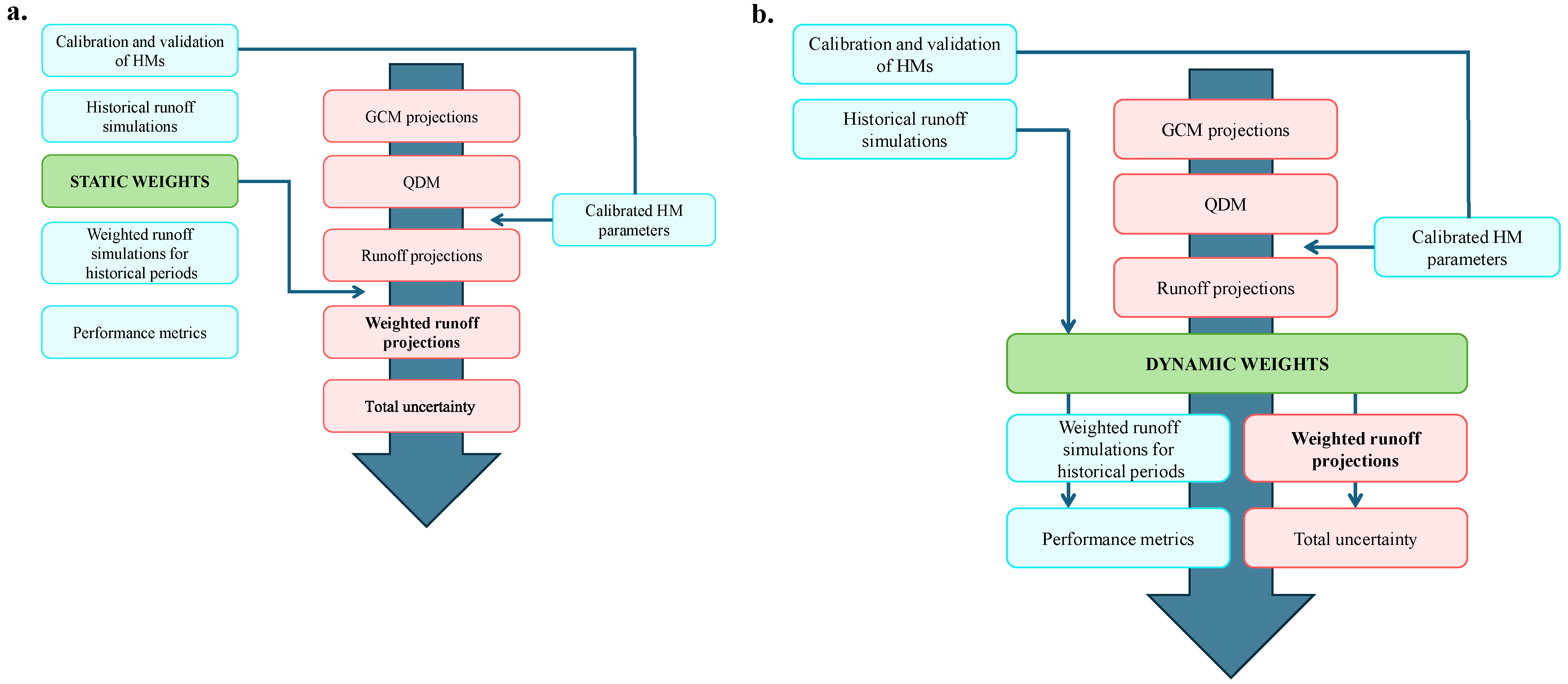
This study builds on the impact modelling chain depicted in Figure 3, focusing on the post-processing step, namely the weighting of runoff projections from multiple HMs. The methods used to evaluate GCM simulations—such as downscaling, bias correction, and uncertainty decomposition—are all essential preprocessing steps, but they have been described in Section 2 as part of the case study setup. Therefore, this section is dedicated solely to presenting the ensemble of HMs and the six distinct weighting methods, which form the methodological core of the study. These components are central to our aim of quantifying the uncertainty in runoff projections.

3.1. Hydrological Models

The employed HMs are calibrated with two main inputs: monthly total precipitation (P) and potential evapotranspiration (PET). While a physically based formula like Penman-Monteith is considered a good choice for PET estimation, it has been recognized that even imperfect PET formulas, which might produce biassed estimations compared to Penman-Monteith, can still lead to robust runoff simulation. This refers to the capability of HMs to compensate for PET differences by parameter adjustments during calibration. Furthermore, it has been highlighted that temperature-based empirical PET formulas tend to perform compatibly with HMs in contrast to more complex formulas needing relative humidity and wind speed [32]. Hence, the PET values used for both the historical period simulations and future projections were derived using the locally calibrated Kharrufa equation, which is based solely on T_mean, as denoted in Table S3.

In this study, seven lumped HMs operating at a monthly time step, previously applied successfully under different changing climatic conditions, are employed (Table S3). The models considered are the abcde model, an extended version of the abcd model with an additional parameter [20]; the Australian water balance model [33]; the dynamic water balance model (Dynwbm) based upon the Budyko framework [34]; the Gr2m model [35], a new version of the Guo model [36]; the Témez model [37], and an improved type of the simple Thornthwaite water balance model (Twbm) [38].

Although employed HMs share a similar conceptual framework, they differ in the mathematical formulations governing the runoff generation (see [20]). While some HMs may include more runoff components than others, those that employ nonlinear functions in generating runoff may enable a more detailed representation of hydrological dynamics. Therefore, weighting all these differently structured models may bring about the potential to enhance simulation capability by using their complementary strengths and making up for their individual limitations.

3.2. Measures for Simulation Performance

Maximization of the Nash-Sutcliffe efficiency (NSE), undoubtedly one of the most widely used criteria for model evaluation [39], was employed as the objective function to calibrate seven HMs over two watersheds. While alternative objective functions exist, parameter sets derived through NSE maximization are consistent in capturing the general aspects of the hydrograph. Having assessed the overall simulation performance during calibration and validation by NSE, the quality of low-flow simulations was additionally evaluated through logarithmic NSE (LNSE), which is computed based on the natural logarithm of runoff values. Since LNSE tends to flatten peak flows, prioritizing low flow conditions at the expense of not being able to represent high flows, it was deemed sufficient for performance evaluation rather than being included as an objective function.

Given that the uncertainty in hydrological projections related to HMs decreased significantly for various indicators following an enhanced calibration procedure [1], our study also prioritized the precise management of the calibration process. Among the numerous automatic optimization algorithms employed for calibrating HMs, the differential evolution algorithm coupled with the Levenberg–Marquardt algorithm was selected because of its relatively rapid convergence to the global optima [20].

3.3. Weighting Methods (WMs)

This study employs six different WMs to obtain reliable runoff projections in the context of climate change (

Table 2. Summary of the hydrological model weighting methods utilized in the study.

Weighting Methods	Negative Weight Possible	Constant Term (w0)	Bias Correction	Iterative	Constrained to Sum to Unity
Equal weight (EW)	X	X	X	X	✓
Bayesian model averaging (BMA)	X	X	✓	✓	✓
Representation of the annual cycle (RAC)	X	X	X	X	✓
Ordered weighted averaging (OWA)	X	X	✓	✓	✓
Granger–Ramanathan (GR)	✓	X	X	X	X
Uncertainty Optimized Multi-Model Ensemble (UO-MME)	✓	✓	✓	✓	X

). As can be seen in Table 2, unlike the developed UO-MME framework, other multi-model averaging methods do not incorporate a constant term in their formulation, and some of the WMs permit the assignment of negative weights to given HMs. The mathematical formulation used to derive the ensemble prediction for month t is presented as follows:

$$Q_{ENS}\left(t\right)=max\left({\sum }_{k=1}^{N_H}{w}_k\times f_k\left(t\right)+w_0,0\right), \forall t,$$

(2)

where Q_ENS denotes the ensemble prediction; N_H represents the total number of HMs considered; w_k signifies the weight assigned to the kth model; w₀ is the constant term; and f_k corresponds to the runoff simulation produced by the kth model.

3.3.1. Equal Weighting (EW)

This approach is rather straightforward, since it assigns identical weights to the predictions of each model in an ensemble. Unlike unequal weighting methods, it disregards the skills of individual HMs and is referred to as a reference approach based on model democracy [2].

3.3.2. Bayesian Model Averaging (BMA)

The BMA aims to integrate multiple predictions from different HMs into a probabilistic streamflow prediction by weighting each of them according to how well it is expected to explain the observed data, depending on posterior probabilities [8,10]. Since BMA operates under the Gaussian assumption of posterior distributions, it is recommended that skewed hydrological data be subjected to Box–Cox transformation before operating BMA. The posterior distribution of the forecast is then expressed as a weighted sum of the individual predictive distributions, where the weights sum to one and are iteratively estimated using the Expectation-Maximization (EM) algorithm. The EM algorithm alternates between computing the expected contributions of each HM for the observed runoff data and iteratively updating the model weights and the corresponding variances. The study performed by Duan et al. [10] provides further details of the BMA.

3.3.3. Representation of the Annual Cycle (RAC)

The representation of the annual cycle (RAC) has been proposed based upon the principles of the Taylor diagram, which incorporates both Pearson correlation (r) and standard deviation ratios to provide a skill score that quantifies the concordance between simulations and observations [17]. The formulation of this index can be expressed as:

$$RAC={\displaystyle \frac{{(1+r)}^4}{{4\left(s+1/s\right)}^2}}$$

(3)

where the parameter s represents the ratio of the standard deviation of monthly runoff simulations to that of the observed data. To estimate the weights, the score indexes regarding the HMs used are normalized to a sum of 1 by dividing each index value by the total sum of all indexes.

3.3.4. Ordered Weighted Averaging (OWA)

The ordered weighted averaging (OWA) method is an operator that weights and fuses predictive data based on a specific performance ranking when there is no precise information about the importance of the weights [40]. Although various algorithms exist to derive OWA weights, one basic approach is a linguistic quantifier, as described below:

$$w_k={\left({\displaystyle \frac{k}{N_H}}\right)}^{\alpha }-{\left({\displaystyle \frac{k-1}{N_H}}\right)}^{\alpha },\hspace{1em}\forall k, \alpha \ge 0,$$

(4)

where greater weight values are assigned to HMs with higher ranks, and α is adjusted to maximize the predictive performance pertaining to ensemble simulations during the calibration period.

3.3.5. Granger–Ramanathan Averaging (GR)

The Granger–Ramanathan averaging (GR) method sets the weights of the simulations considered in the ensemble via the ordinary least squares (OLS) algorithm [41]. It offers advantages in hydrological applications as an unconstrained method, since the estimated weights do not necessarily sum to unity, and it may allocate negative weights to HMs. The methodological details of the GR method have been extensively discussed in Castaneda-Gonzalez et al. [3] and Diks and Vrugt [11].

3.3.6. Uncertainty Optimizing Multi-Model Ensemble (UO-MME)

The methods described above generally assign weights to the HMs based on their historical simulation performances. These weights are preserved in a static way (Figure 4a) and then integrated into climate projections, as in existing studies (e.g., [2,3,9]). However, weights that produce satisfactory simulations during historical periods neither guarantee a realistic representation of future climate change signals nor promise a reduction in uncertainty. These concerns underline the necessity of a balanced scheme that reduces the uncertainty variance in weight-driven hydrological projections and performs in accordance with past conditions. In line with this rationale, the UO-MME framework (Figure 4b) evaluates the trade-offs between the changes in simulation performances during the observation period and the projection uncertainties and dynamically optimizes the weights assigned to HMs using a multi-objective evolutionary algorithm, the non-dominated sorted genetic algorithm II (NSGA-II).

NSGA-II is such an elitist and fast approach to successfully solve cases with two objectives [42]. Therefore, it undertakes the objectives of maximizing NSE during the calibration period and optimizing the long-term mean total projection uncertainty over 2021–2099, defined in terms of the notion of variance (Equation (5)).

$$mT{U}_{3way}={\displaystyle \frac{1}{n_T}}\sum _{t=1}^{n_T}\left({\displaystyle \frac{1}{n_R\times n_G\times n_D}}\sum _{e=1}^{n_R}\sum _{g=1}^{n_G}\sum _{d=1}^{n_D}{\left[{∆qw}_{e,g,d}\left(t\right)-{∆qw}_{o,o,o}\left(t\right)\right]}^2\right)$$

(5)

where ∆qw represents the mean runoff change derived from runoff projections based on HM weighting. Specifically, ${∆qw}_{e,g,d}\left(t\right)$ expresses the change associated with a given RCP scenario e, GCM g, and downscaling method d at year t. The definitions of n_R, n_D, and n_G are the same as those provided in Equation (1). The analysis spans n_T = 79 years, while ${∆qw}_{o,o,o}\left(t\right)$ denotes the overall average of the computed changes, obtained by considering all variations at year t.

Both objective functions, which are NSE and mTU_3way (see Equation (5)), were addressed through Pareto front analysis, achieving a balance between competing trade-offs. The developed framework also enables negative weighting and adaptably identifies the contributions of multiple HMs, which is in line with a scant number of papers emphasizing the superiority of unconstrained weighting methods over constrained ones (e.g., [8,11,12]). The potential of UO-MME to narrow the uncertainties propagated across the four-factor modelling chain—including HMs—compared to conventional WMs is discussed in Section 4.3.2.

Of course, we are aware that the absolute ‘true’ uncertainty of future runoff cannot be known, and uncertainty-integrated variants of BMA (e.g., [43]) or other well-known methods could be formulated as well. However, we aim not to portray UO-MME as superior in reflecting the ‘true’ future, but rather to investigate how ensemble behaviour changes under different weighting types and to introduce a simple yet multi-objective framework that allows users to balance simulation performance and projection spread. Instead of conducting a perfect model experiment (PME), where the ‘true’ response is known by a model-designated reference simulation (e.g., [44]), our work offers an operational ensemble framework aligned with comparative applications in the recent literature, in which the objective of reducing uncertainty in runoff projections has been acknowledged as a critical step toward more decision-relevant hydrological modelling (e.g., [19,45,46]).

4. Results and Discussion

4.1. Simulation Performance of HMs

This section has assessed the simulation capabilities of various HMs in two distinct watersheds by utilizing NSE and LNSE metrics (Table S3). While HMs yielding higher NSE values are regarded as more reliable as they pertain to their overall performance, LNSE offers additional evidence to help evaluate their credibility during low flow periods. It is clear from Table S3 that the majority of HMs employed for the Beydag watershed are classified as good in terms of NSE performance during the calibration period, as per the performance ratings provided by Moriasi et al. [47]. Although some HMs are rated as very good for the validation data for the Beydag watershed, Dynwbm demonstrated superior performance in both the calibration and validation phases by better capturing the overall shape of the hydrograph.

Additionally, since all the HMs calibrated for the Tahtali watershed generated a runoff simulation classified as very good, it is likely that the rainfall-runoff relationship could be more readily established in this study region. For instance, unlike the relatively poorer calibration performance of Gr2m in the Beydag watershed, its plausible results for the Tahtali watershed suggest that less detailed conceptualization may also be appropriate in cases where calibration is supported by sufficient data. Given that a minimum of 10 years of data is recommended for the reliable calibration of monthly rainfall-runoff models [48], the relatively short record length of natural flows in the Beydag creek may have resulted in slightly lower simulation performance in this region.

Furthermore, when HMs in the Beydag watershed were calibrated to optimize NSE, they often showed unsatisfactory LNSE performance, as this objective function can prioritize higher flows that contribute more notably to the overall variance; nevertheless, Dynwbm steadily outperformed the other HMs in terms of LNSE there. In contrast, its ability to capture low flows in the Tahtali case is somewhat poorer (LNSE < 0), while certain HMs (i.e., Twbm and abcde) stand out in the validation data by effectively maintaining the overall NSE-LNSE balance. That is, all these findings generally disclose that the simulation performances of HMs may vary according to hydrological regimes and data length as well. Given these findings, it is, of course, intriguing to reveal the real contribution of HMs to the total uncertainty in runoff projections. But examining the effects of weights assigned to HMs on runoff projections would become even more essential, regardless of whether the response of the HM selection to the total uncertainty is marginal or not.

4.2. Projected Changes in Runoff

In this section, we analyzed an ensemble of 140 runoff projections obtained through the chain combination scheme illustrated in Figure 3. For each HM, changes in the annual mean runoff (ΔQ_m) over twenty-year periods in the GCM-driven runoff projections were computed relative to the mean values of the HIST simulation for the corresponding GCM. Accordingly, the projected ΔQ_m values are shown in Figure 5 and Figure S3 for the Beydag and Tahtali watersheds, respectively. The statistical significance of these changes and the quantification of uncertainty, analyzed based on variations between sources, are separately discussed in Section 4.2.1 and Section 4.2.2, respectively.

4.2.1. Statistical Significance of Changes

A collective examination of Figure 2, Figure 5 and Figure S3 shows that even minor reductions in precipitation can have a marked impact on ΔQ_m in these water-stressed watersheds (e.g., the changes projected by GFDL-SD over the period 2060–2099 under RCP4.5). The influence of substantial precipitation decreases on runoff has, unsurprisingly, been even more dramatic. For instance, under RCP8.5, the significant precipitation decreases projected by GFDL as of 2060 may bring about runoff reductions in the Beydag and Tahtali watersheds, ranging from [−33%, −74%] and [−27%, −63%], respectively. As stated in Section 2.2.1, the HadGEM-CRX projected atypical increases in both precipitation regime and temperatures over the Beydag watershed under the RCP8.5. As expected, the runoff was mainly influenced by precipitation variability in this case, resulting in notably wetter conditions. In addition, under the same emission scenario for the Beydag watershed, the fact that HadGEM-SD and HadGEM-CRX projected runoff changes in the range of [−18%, −38%] and [+12%, +59%], respectively, during the period 2021–2099 underscores that DM uncertainty may gain relative importance when relying on a single GCM. Given that climate elasticity of runoff was more driven by projected changes in precipitation, the patterns in Figure 5 and Figure S3 may provide a preliminary understanding that the uncertainty in projected runoff is mostly attributable to the uncertainty in the GCM-driven precipitation projections.

Moreover, both the magnitude of ΔQ_m and their statistical significance by Dunnett’s test across variants differ between the two cases. Very few of these changes are in the direction of increase. In the Beydag watershed, roughly half of the variants suggest statistically significant decreases. This proportion is about one-third for the Tahtali watershed. Anomalies in both regions tend to intensify over time and undergo clear shifts starting from 2060. In addition, the slightly more pronounced changes in the Beydag case may make its reservoir more vulnerable to the effects of climate change.

When evaluated based on HMs, Awbm and Twbm exhibit the most marked decreasing runoff trends for both watersheds, whereas the Guo model may have made the GCM-derived outputs less significant and showed somewhat lower sensitivity to changing climate. Although Twbm strikes a balance between the measures for the Tahtali watershed, its limited capability to achieve a similar performance in the Beydag watershed may have escalated the runoff reductions there.

Accordingly, GFDL is the GCM that has projected a statistically significant decrease in the most variants in both watersheds, and other GCMs present varying anomaly responses across the watersheds (see Figure 5 and Figure S3). For example, while MPI displays statistical significance in two-thirds of the variants in the Beydag watershed, only one-fifth do so for the Tahtali watershed under this GCM. In addition, CNRM resulted in statistical significance being observed in a very limited number of variants (7%) for the Tahtali watershed; yet, surprisingly, the frequency of statistically significant decreases projected by the same GCM reached 40% for the Beydag watershed. These findings highlight the strong dependence of runoff projections on how multi-GCM combinations are constructed over a specific study area and which emission scenarios they interact with, as already raised by Wang et al. [49].

4.2.2. Partitioning Uncertainty in Runoff Projections: Four-Way ANOVA

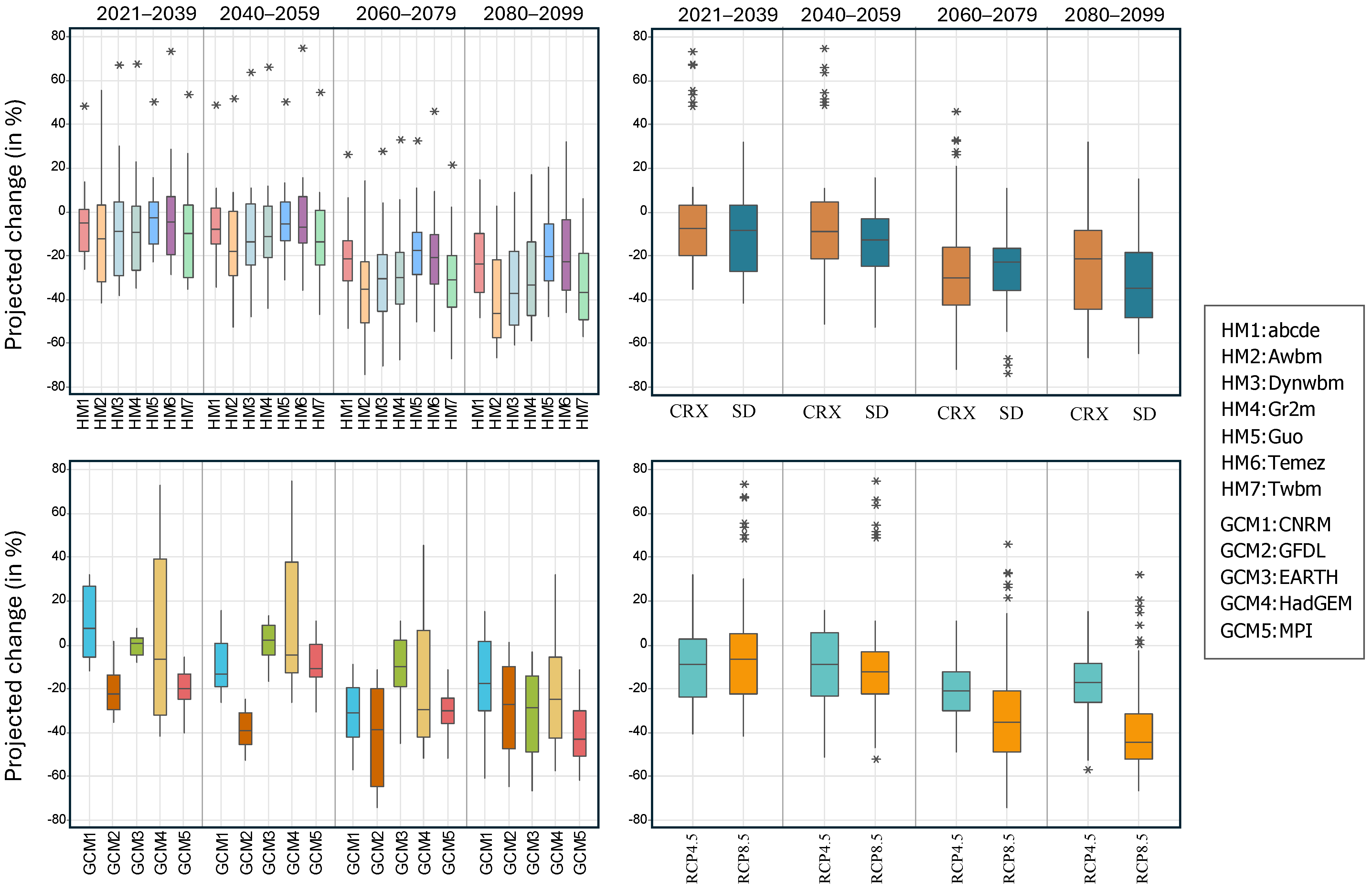
All potential anomaly combinations compiled for a certain source within the modelling chain are presented using the box-whisker plots in Figure 6 as an example for the Beydag watershed. While this figure improves the readability of Figure 5 and provides a preliminary insight into the temporal uncertainties of variations, decomposing the total uncertainty for ΔQ_m using four-way ANOVA has deciphered the real contributions of the sources (Figure S2). Using this approach, the total variance can be partitioned into 15 components, including four main effects, six second-order interactions, four third-order interactions, and one fourth-order interaction involving all factors [30]. For ease of interpretation, Figure S2 displays the total contribution of all interaction effects combined. Accordingly, it has been observed that the uncertainty contribution caused by HM selection is marginal (~1–2%) and even lower than the uncertainty associated with emission scenarios. Even so, it should be noted that the low quantification of the uncertainty mentioned herein implies that the relative contribution of the ensemble of anomalies derived from the employed HMs is limited, as also emphasized for mean flows by Feng and Beighley [30]. Certainly, biases in downscaled GCM data are propagated nonlinearly through hydrological modelling uncertainties—such as model structure and parameter estimation—ultimately amplifying the overall uncertainty spread, as stated by Duan et al. [9].

The fact that the uncertainty in runoff projection governed by HMs is significantly larger than that of precipitation in terms of the variance for both watersheds verifies that the uncertainty inherited from the downscaled data is further distorted through hydrological modelling. Given that it has been previously determined that hydrological model parameter uncertainty can become a negligible factor within the combination chain due to being overshadowed by the huge GCM uncertainty (e.g., [50]), it is considered that the spread of uncertainty in ΔQ_m is more influenced by the structural characteristics of HMs, such as runoff generation and actual evapotranspiration mechanisms. While Najafi et al. [6] emphasized that an HM with the simplest structure among the others has exhibited the highest GCM uncertainty, contrary situations can take place in our study. Specifically, Dynwbm, which incorporates nonlinear quick flow and actual evapotranspiration components, and demonstrates more robust simulation performance in the Beydag watershed, was found to act as a lens that disproportionately amplifies GCM-driven input uncertainties (see the panel in the upper left corner of Figure 6).

As seen in Figure 2, anomaly differences emerged depending on the DM selection in some variations, likely due to biassed signals generated by excessive RCM parameterization in certain grids or the underestimation tendency of SD. But notwithstanding, either the use of a multi-source ensemble or subjecting each DM output to the same bias correction procedure may have helped to balance systematic errors from individual DM and projection biases specific to a single GCM. Moreover, although the interaction between GCMs and other sources has been omitted in some studies (e.g., [51]), it is observed that, on average, 40–55% of the total uncertainty is accounted for by the sum of the first- and second-order interactions of GCMs with RCPs and DMs, despite their temporal fluctuations. As also observed in precipitation projections, the largest share of this uncertainty belongs to the GCM-RCP interaction. Even though the contribution of RCP selection to uncertainty increases slightly over time (Figure S2), it remains equivalent to the proportion measured for precipitation, roughly 10%. It is also apparent from the results that the integration of specific GCMs with different sources resulted in prominent uncertainties in specific periods. For instance, HadGEM projected a notably wider interquartile range compared to other GCMs until the end of the 2050s. It was seen in later periods that GFDL was found to give as much uncertainty as HadGEM, and even in the Tahtali watershed, more elusive patterns emerged. As a result of these findings, it is evident that, for ΔQ_m, GCM selection was the second most influential factor after total interaction and contributed 30–40% to total uncertainty.

4.3. Multi-Hydrological Model Weighting and Potential Impacts on Uncertainty

Unravelling the root causes of disparities in runoff projections due to structural uncertainties in GCMs and HMs is beyond the scope of this study. Instead, we applied different weighting techniques to the outputs of HMs driven by GCM-derived data to narrow uncertainty and optimize HMs’ contributions, thereby obtaining more reliable runoff projections.

4.3.1. Simulation Performance Versus Projected Uncertainty in Standard WMs

Using simulated runoff series from seven ensemble members for the calibration period, we first evaluated constrained WMs, which satisfy the sum to unity condition, and then estimated weights were applied to both the validation period and future projections. It can be seen from

Table 3. Weights assigned by different WMs and their corresponding NSE and LNSE scores. The results for the Beydag and Tahtali watersheds are presented in panels (a) and (b), respectively. Weights w₁ to w₇ have been assigned following the HM order given in Table S3.

(a)		w0	w1	w2	w3	w4	w5	w6	w7	NSEcal	NSEval	LNSEcal	LNSEval
	Constraint methods
	EW	-	0.143	0.143	0.143	0.143	0.143	0.143	0.143	0.754	0.798	0.412	0.409
	BMA	-	0.156	0.127	0.183	0.140	0.126	0.118	0.151	0.760	0.802	0.423	0.419
	RAC	-	0.147	0.137	0.162	0.137	0.132	0.135	0.150	0.757	0.799	0.416	0.413
	OWA	-	0.045	0.033	0.783	0.019	0.022	0.027	0.071	0.793	0.800	0.563	0.557
	Unconstraint methods
	GR	-	0.603	−0.143	0.629	−0.135	−0.317	0.000	0.359	0.804	0.814	0.668	0.685
	DP1	0.430	0.646	−0.251	0.788	−0.413	−0.031	−0.240	0.498	0.792	0.798	0.664	0.658
	DP2	0.501	0.647	−0.266	0.727	−0.377	−0.006	−0.268	0.504	0.794	0.792	0.653	0.642
	DP3	0.576	0.673	−0.279	0.712	−0.403	0.130	−0.388	0.509	0.789	0.788	0.648	0.632
	DP4	0.646	0.674	−0.294	0.650	−0.367	0.156	−0.416	0.515	0.786	0.776	0.628	0.612
	DP5	−0.017	1.585	−0.118	0.335	−0.747	−0.483	0.182	0.309	0.755	0.790	0.601	0.746
(b)		w0	w1	w2	w3	w4	w5	w6	w7	NSEcal	NSEval	LNSEcal	LNSEval
	Constraint methods
	EW	-	0.143	0.143	0.143	0.143	0.143	0.143	0.143	0.855	0.921	0.838	0.892
	BMA	-	0.163	0.137	0.111	0.181	0.096	0.118	0.193	0.856	0.922	0.840	0.896
	RAC	-	0.144	0.146	0.138	0.145	0.144	0.137	0.144	0.855	0.921	0.839	0.894
	OWA	-	0.084	0.582	0.047	0.124	0.055	0.042	0.066	0.860	0.907	0.850	0.913
	Unconstraint methods
	GR	-	0.559	1.256	−0.113	−0.088	0.151	−0.076	−0.689	0.866	0.901	−0.341	0.154
	DP1	−0.037	1.163	−0.298	−0.174	−0.276	0.222	0.397	−0.045	0.835	0.898	0.805	0.858
	DP2	0.077	1.161	−0.224	−0.142	−0.404	0.187	0.407	−0.134	0.804	0.873	0.811	0.861
	DP3	−0.234	1.742	−0.482	−0.310	−0.578	−0.570	0.402	0.716	0.815	0.873	0.809	0.863
	DP4	0.128	1.226	−0.536	−0.169	−0.290	0.323	0.405	−0.046	0.812	0.881	0.796	0.849
	DP5	−0.214	1.910	−0.541	−0.436	−0.603	−0.547	0.405	0.726	0.810	0.857	0.807	0.862

Notes: The subscripts cal and val denote the performance values obtained for the calibration and validation data, respectively. The most suitable result for each performance metric is highlighted with underlining.

that the RAC method performed similarly to EW and presented a pattern that almost shows a model democracy. This suggests that information provided from the Taylor diagram, which relies on descriptive statistics such as Pearson correlation instead of NSE, may not be sufficiently discriminatory for the weighting process. In addition, it was observed that BMA assigned a slightly higher weight to the Dynwbm model, which achieved the highest NSE score during the calibration period in the Beydag watershed. However, the poor performance of this model under low-flow conditions in the Tahtali watershed may have caused constrained WMs to assign it relatively lower weights. Consistent with the findings of Darbandsari and Coulibaly [52], it is also seen that BMA weights are not completely in accordance with individual HM performances, as relatively low-performing HMs can receive higher weights, and vice versa.

On the other hand, the OWA assigned weights exceeding 0.50 to Dynwbm in the Beydag watershed and AWBM in the Tahtali watershed while demanding minor contributions from the remaining HMs used (Table 3). Hence, it can be said that the OWA method largely adhered to the ‘strict weighting’ advocated by some studies to ensure more reliable runoff projections (e.g., [1]). This weighting strategy, which reduced model diversity within the ensemble and led to lower weighting entropy, resulted in slightly improved simulation performance during low flow periods compared to other constrained WMs. Even so, neither this method nor the remaining constrained WMs demonstrated a marked overall superiority over the best-performing HMs.

As for the unconstrained method GR, it exhibited different simulation responses between the two watersheds (Table 3). In the Beydag watershed, its weights generally favoured the model rankings according to NSE scores, while in the Tahtali watershed, despite the HMs having relatively similar NSE values, GR has assigned significantly different weights, including larger negative values to certain HMs. This is likely because GR is based upon the OLS algorithm, which can introduce negative-weighting instances that moderate the influence of some HMs in the final ensemble estimate. Even though GR-based weighting provided the highest NSE during the calibration period, demonstrating superior performance over both the four constrained WMs and any sole HM, this improvement remained marginal compared to previous works where GR showed clear performance gain (e.g., [8,11]), and it even led to adverse LNSE results during the validation period for the Tahtali watershed.

All these observations highlight that WMs aiming to compensate for model errors may not improve performance in every case across all flow conditions. As one might attribute this limited improvement in simulation performance to the number of ensemble members, the use of seven HMs in this study still lies within the acceptable range suggested by Wan et al. [12], who found ensemble sizes between 6 and 9 to be enough for reliable multi-model combination performance. Overall, the findings of our study point out that the merits of standard WMs may vary across hydrological regimes; at the same time, it is important to note that even methods such as GR that provide consistent simulation performance could have a significant impact on the magnitude of hydrological projections, as reported by Castaneda-Gonzalez et al. [3], thus warranting further investigation into their limitations. So, this section intimately investigates the extent to which the decomposed uncertainty in runoff projections is affected by the inherent functioning of all these standard WMs and their past simulation performance. Pastén-Zapata et al. [2] stated that the impact of WM choice on reducing runoff projection uncertainty can vary depending upon the purpose-specific metrics (e.g., projected mean annual flow, low flows, etc.). However, since the HMs used are monthly water balance models, which may not capture high and low flows as robustly as daily scale models, our WM examination has centred only on temporal uncertainty decomposition for projected changes in annual mean streamflow (ΔQ_m).

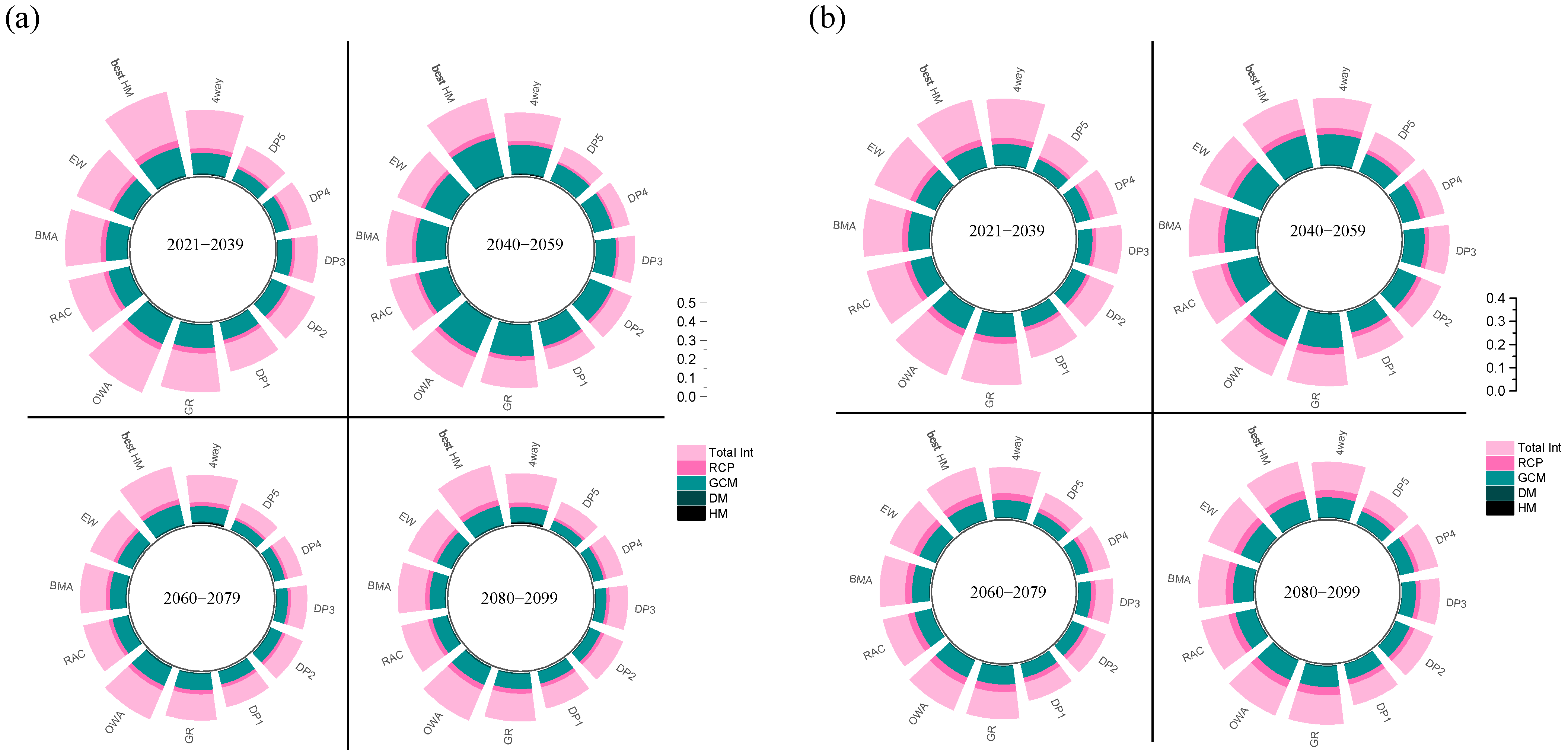
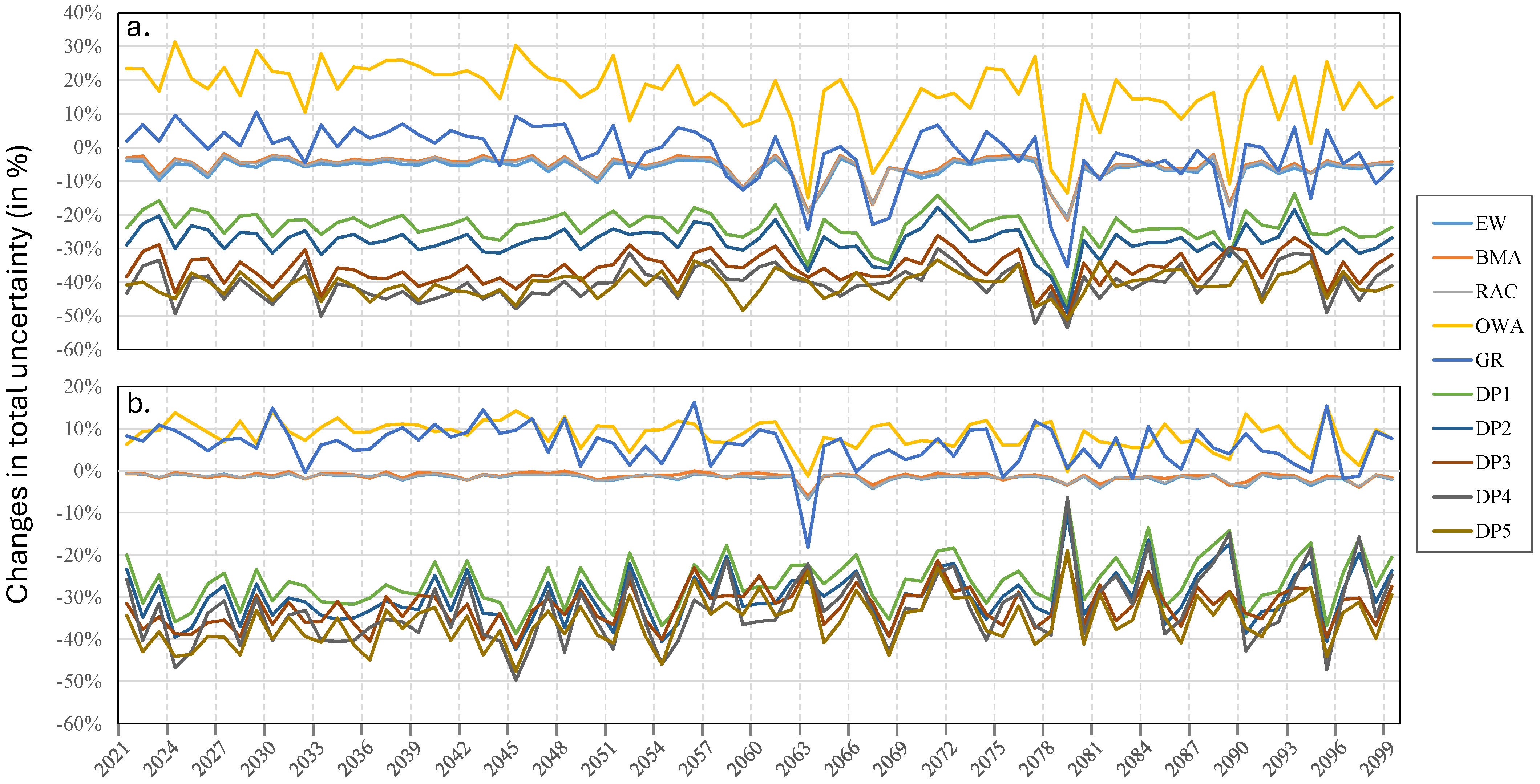
As shown in Figure 7, individual HMs that performed well overall (i.e., best HMs) exhibited apparent sensitivities to GCMs and GCM-RCP interactions, likely due to their internal structure, and thus, weighted combinations were expected to alleviate such variability. But there were particular variants where the decomposed variance patterns from static WMs differed significantly from one another. Although the variances derived from the full modelling chain involving seven HMs were lower than those of the best-performing HMs, the extent to which further uncertainty reductions could be made by HM weighting would be even more essential. Accordingly, the changes in uncertainty variances derived through the different WMs were evaluated with reference to the four-way ANOVA results. The changes in total variance associated with HM weighting are presented in Figure 8, while Figure 9 illustrates the corresponding changes for some of the key sources contributing most significantly to total variance, namely GCMs and their interactions with other main factors. However, since the ANOVA framework used does not separate stochastic year-to-year fluctuations from interaction effects, the variance attributed to interaction may partially reflect internal variability. While properly isolating such contributions is beyond the scope of this study, the primary focus has been on whether ‘overall’ uncertainty can be reduced by HM weighting.

In addition, it is immediately obvious from these figures that the similar distributions of weights assigned to HMs by the RAC, EW, and even BMA methods have led to similar contributions to uncertainty reduction, which remain marginal, regardless of temporal span, with decreases limited to 4–6%. Although some studies have stated that discarding low-performing HMs from the candidate multi-model ensemble prior to weighting may reduce projection uncertainty by preserving overall effectiveness [1,6,7], the results obtained through OWA, which to some extent resembles a strict weighting analysis, unexpectedly pointed to the opposite, with projection uncertainty during the 2021–2099 period increasing by nearly 20% in the Beydag watershed and 9% in the Tahtali watershed. Another important finding is that although GR allows for the assignment of negative weights to HMs—thus potentially capturing the covariance structure among simulation errors—this does not necessarily make it a more credible WM for impact assessment, since its contribution to uncertainty change in the Beydag watershed was neutral in the long term, whereas in the Tahtali watershed it even increased runoff projection uncertainty, almost to the extent observed with OWA (see Figure 8).

When simulation performance among HMs differs meaningfully, the change in runoff projection uncertainty has been shown to be influenced by the weighting scheme [2]. But, in our study, all HMs receive either good or very good ratings in terms of NSE, and hence, pursuing additional efforts to enhance simulation performance for the multi-model ensemble using standard WMs may not result in further reductions in projection uncertainty (Figure 7, Figure 8 and Figure 9). Moreover, as highlighted by Coron et al. [53], the HMs that perform well under current climate conditions cannot guarantee robust results under future climate scenarios; therefore, statically weighting such models based solely on their historical performance can still be subject to the same limitations. Perhaps understanding how the internal mechanisms of HMs (i.e., runoff generation components) contribute to total uncertainty in our case studies, rather than treating HMs as individual entities, could have offered a pathway for uncertainty management. However, since addressing this issue lies beyond the scope of this study for now, adopting an alternative weighting approach that aims to balance the variability in HMs’ responses to GCM-derived climate signals appears to provide a more straightforward framework.

4.3.2. Does the UO-MME Framework Effectively Reduce Projection Uncertainty?

Some HMs may lead to underestimated runoff projection uncertainty because of their inability to represent hydrological processes adequately for the sake of simplicity, as emphasized by Pastén-Zapata et al. [2]. Conversely, as observed in Figure 6 and Figure 7, HMs exhibiting high simulation performance under historical conditions may show larger responses to projected climate change signals, possibly due to structural limitations or some parameterization choices, thereby inflating projection variance. These situations appear to pose challenges to standard weighting methods when optimizing the influence of HMs on runoff projection uncertainty. In other words, their ability to achieve the dual goal of providing reasonable historical simulation accuracy while reducing projection uncertainty may be limited. It was precisely these observations that motivated the application of the UO-MME approach, and herein it was tested whether it could circumvent these limitations.

The NSGA-II algorithm, driving the UO-MME framework using a population size of 50, was observed to converge after 100 iterations, subsequently yielding the Pareto frontiers shown in Figure S4. From this figure, the trade-off between NSE-based simulation accuracy and long-term mean total projection uncertainty is obvious for both watersheds. Some points within this trade-off space offer steadily reduced projection uncertainty in return for accepting up to a 5% decrease in NSE for the calibration data compared to that of the best-performing HM. However, even amongst these, certain points still failed to provide sufficient LNSE values. Therefore, despite the analysis being structured as a bi-objective evaluation, decision point selection favoured solutions in which LNSE remained above given thresholds, specifically LNSE > 0.60 for the calibration data in the Beydag watershed and LNSE > 0.75 in the Tahtali watershed, thus forming a refined subset of Pareto-optimal solutions.

Ultimately, five decision points (DP1 to DP5) were identified as optimal candidates for each watershed, since they provided both robust historical simulation performance and a meaningful reduction in projection uncertainty. Accordingly, this dynamic framework operates as a post-processing refinement of hydrological projections, similar in spirit to methods that adjust uncertain model states in the presence of noisy forcing data (e.g., [43]). The weight estimates derived from the UO-MME approach, along with the associated NSE and LNSE performances of these decision points, are presented in Table 3. The corresponding levels of projection uncertainty and their changes relative to those of the four-way ANOVA are illustrated in Figure 7, Figure 8 and Figure 9.

As observed in Figure 8, while the magnitude of projection uncertainty reduction slightly intensifies from DP1 to DP5, both watersheds exhibit a comparable pattern in terms of the range of reductions, with average values between 25% and 40%. The patterns of uncertainty change obtained with UO-MME imply that the direction of change remains continually negative over 2021–2099 and confirm that a more systematic uncertainty management strategy could be established compared to WMs such as RAC, BMA, and EW, which result in close to zero or only marginal uncertainty reductions. Although the primary target of this study was not to select the best decision point, a comparative analysis of the five alternatives for each watershed suggests that DP3, which likely provides a better positive-negative weight balance, offers a well-balanced compromise between maintaining simulation capability and narrowing projection uncertainty. That is, the DP3 preserved ensemble simulation quality by assigning relatively higher weights to the best-performing HMs (i.e., w₃ and w₇ for the Beydag and Tahtali watersheds, respectively) and attempted to extract useful information from lower-performing HMs as well, in line with Darbandsari and Coulibaly [52] and Castaneda-Gonzalez et al. [3]. It even allocated more controlled negative weights to certain HMs when needed, thereby achieving a well-structured trade-off. As shown in Table 3, DP3 provided consistent simulation performance in the Beydag watershed, with an NSE of 0.79 and an LNSE close to 0.65 during both the calibration and validation periods. In addition, the results were even more robust for the Tahtali watershed, where all NSE and LNSE values exceeded 0.80, verifying credibility across all evaluation periods.

Another key finding from our study is that the change in total uncertainty is mostly governed by adjusting the variance from GCMs and their interactions with other sources (see Figure 9). It should be acknowledged, however, that the UO-MME framework does not directly reduce the structural uncertainty of GCMs themselves, as such uncertainty stems from inherent modelling differences in representing the physical processes of the climate system. Instead, it undertakes to balance the effects of climate signals produced by GCMs that are reflected in the projections through HMs. For instance, using DP3, the long-term average reduction in GCM uncertainty over the 2021–2099 period was nearly 28% for both watersheds, which was made possible by tempering the hydrological response of HMs to GCM-derived signals to some extent through controlled weighting. Moreover, it was noted that the intensity of GCM uncertainty reduction in the Tahtali watershed was slightly lower during the 2060–2099 period compared to earlier spans. All these imply the need for alternative schemes to those in previous studies (e.g., [5]), which base HM weighting solely on historical simulation skills to reduce projection uncertainty.

Pastén-Zapata et al. [2] revealed that a greater spread in model weights leads to a greater uncertainty reduction, and this seems generally valid for the UO-MME results. On the contrary, methods like OWA and GR—despite producing higher standard deviations among weights—often failed to reduce uncertainty and, in most cases, even amplified it. For example, during the 2080–2099 period, the adopted approach achieved average reductions in GCM-related uncertainty ranging between 20% and 34% for both watersheds, whereas the standard methods either produced neutral effects or led to undesirable increases in variance, as shown in Figure 9. According to Castaneda-Gonzalez et al. [3], the contrast between the mean climate of the calibration period used by HMs and that of the climate projections can vary depending on the GCM–RCP pairings. Hence, the contrasting conditions that are likely to have occurred with the GCMs used in our study may have also affected the way structural uncertainties in HMs respond over years, leading to different trajectories of GCM uncertainty propagation, irrespective of the weighting scheme used.

As similarly observed, under the UO-MME framework, inter-period differences in the magnitude of uncertainty change generally stayed within a ±5% range. An exception was detected for the Tahtali watershed, where nearly 10% less uncertainty reduction was obtained for the 2060–2079 period compared to the preceding twenty-year span. These patterns are likely because, in both UO-MME and other WMs, the weights assigned to HMs remain constant throughout the projection period, which may dampen the fluctuations in the temporal dynamics of uncertainty change. Although UO-MME does not implement temporal variation in weights (see Table 3), it may still be regarded as a dynamic weighting approach, since it considers each GCM–HM combination individually and partially suppresses the influence of certain HMs that contribute more to the projection uncertainty despite their high historical performance by allocating appropriate weights to the remaining ensemble members.

It is also seen in Figure 7 that not only the uncertainty variances associated with all WMs, but also those of the best-performing HMs, are relatively larger during the earlier windows (2021–2039 and 2040–2059). Even under reduced projection uncertainty achieved through the UO-MME approach, the variance attributed to GCMs during the 2021–2059 period remained markedly greater than that of the 2060–2099 period, by roughly 55–65% in the Beydag watershed and 18–30% in the Tahtali watershed, across different decision points of UO-MME. Although temperature projection uncertainty tends to be considerably higher in the late windows (2060–2079 and 2080–2099), the relatively lower runoff uncertainty during these periods is essentially driven by the imprint of the precipitation signal on runoff responses (Figure S2). That is, the greater total projected runoff uncertainty in the earlier windows compared to the late windows is likely not attributable to the employed weighting scheme but instead reflects the interannual variability in precipitation as simulated by the GCMs. Although such patterns are not always discussed in the literature, our results can be considered consistent with the findings of Taguela et al. [54]. This is likely because they pointed out that the influence of internal variability in projected precipitation diminishes as lead times increase and plays an important role mostly for the near-term periods. Additionally, streamflow projections also show non-monotonic patterns of uncertainty propagation over years, as noted by Najafi et al. [6]. As in our study and other ANOVA-based applications (e.g., [15,29,30]), interaction terms may have implicitly involved the effect of internal variability because interannual fluctuations were not explicitly decomposed by a time-series-based ANOVA technique. While Yip et al. [31] quantified the contribution of internal variability to total uncertainty in climate projections using different initial condition ensemble members for each model and scenario, we considered the GCM simulations with a single initial condition only (i.e., mostly r1i1p1f1). Therefore, we acknowledge this as a limitation and note that disentangling the stochastic and deterministic components of interaction terms remains a methodological challenge for future research.

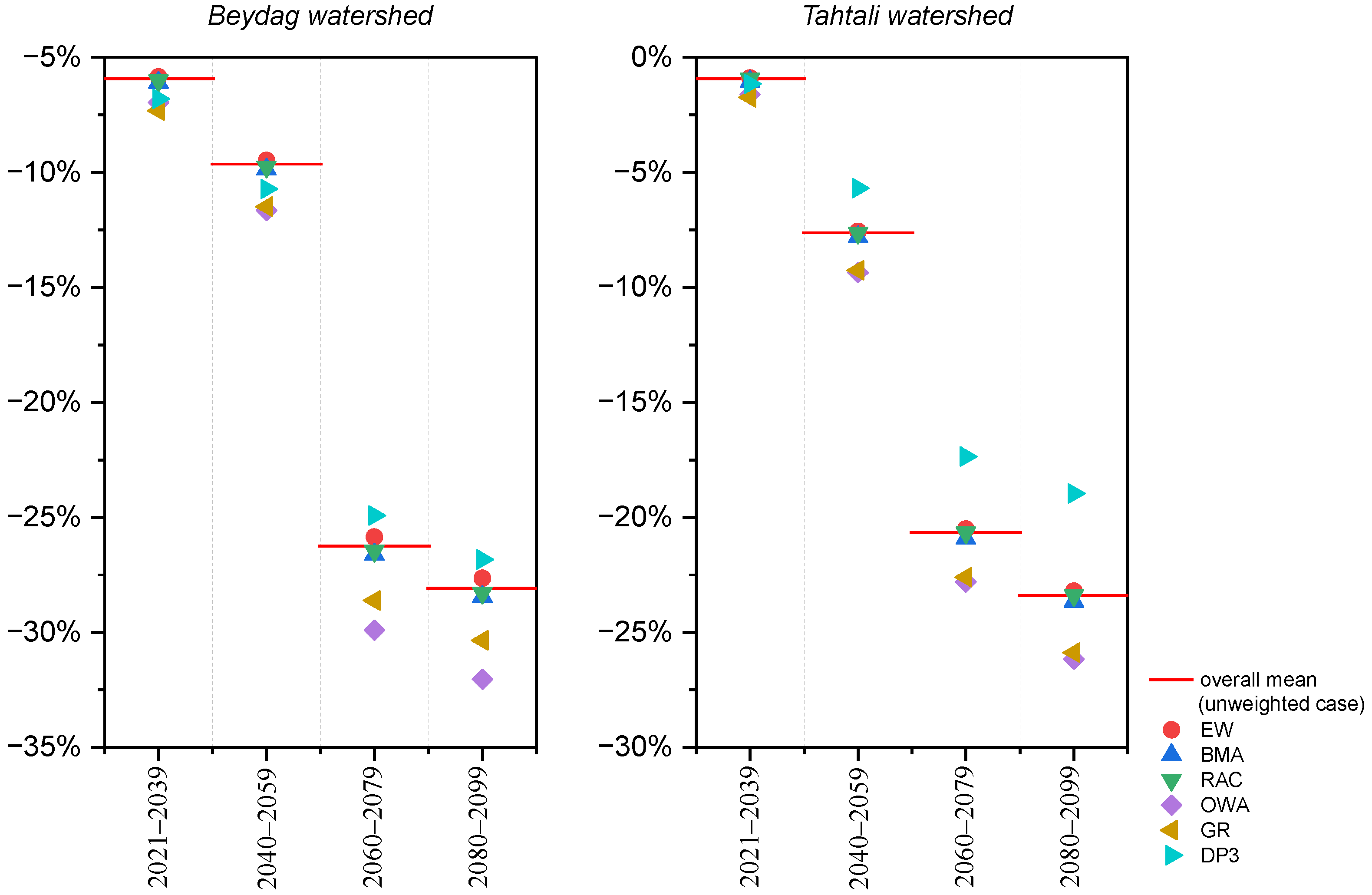
Moreover, the WMs employed are not only expected to change projection uncertainty but also inevitably influence the central tendency of hydrological change estimates. To illustrate this, ΔQ_m values for the related future spans were derived by averaging 140 ensemble members for the unweighted case and 20 ensemble members for each WM. Figure 10 verified that WMs jointly project a decrease in annual mean streamflow during all future periods for the Beydag watershed. These reductions rise over time, with changes around 6–12% in the earlier windows, reaching up to 32% in the late windows. In the Tahtali watershed, similar temporal patterns emerge, though with slightly lower magnitudes, and those decreases range from about 1–9% in the earlier windows to 17–26% in the late-century projections. In addition, GR and OWA, which increased projection uncertainty, produced the largest runoff decreases in both watersheds, especially in the late windows, while DP3, which avoids strict weighting over several well-performed HMs, produced slightly less runoff reduction. The trade-off inherent within UO-MME-based weighting that allows some compromise in simulation performance (i.e., NSE) to obtain greater reductions in projection uncertainty appears to have resulted in these relatively smaller runoff decreases.

The results mentioned in this section unequivocally show that the magnitude of projection uncertainty variance is sensitive to the choice of weighting scheme and can be mitigated by UO-MME, which does not solely consider the performance-dependent weighting. Nevertheless, the relative proportions of variance across time windows and the fractional contributions of different sources to overall uncertainty remained quite similar (see Figure S5). It was seen that, on average over the entire projection period, GCMs contributed roughly one-third to the overall runoff uncertainty, while almost half of the total variance was attributed to the possible interactions among all contributing factors, which is in line with other studies (e.g., [15,29,32]). Because bias correction alone can significantly reduce the uncertainty associated with GCM data (see also [51]), the contribution of HM weighting should be interpreted as a further step towards fortifying the credibility of runoff projections.

5. Conclusions

This study seeks to determine the extent to which different hydrological model weighting schemes contribute to narrowing the uncertainty in runoff projections. Just as HMs that are classified as good to very good under current climate conditions may not ensure robustness under future climate scenarios, statically weighting them based on historical skills alone may not always make a meaningful contribution to reducing projection uncertainty. The results show that using a more extensive set of HMs does not decrease ensemble predictive skill and that additional information can be extracted from lower-performing HMs with a view to tempering total uncertainty, unlike OWA, which behaves as a strict weighting approach. OWA and GR imposed more distinct weighting patterns, which slightly increased simulation skill during the observation period but, in some cases, noticeably inflated the amount of uncertainty. Despite being flexible, other standard methods, such as BMA and RAC, produced weight distributions quite similar to EW and delivered only marginal reductions in projection uncertainty (<5%). Motivated by these findings, the UO-MME framework optimizing model weights under a bi-objective structure was adopted. A decision point from the Pareto front achieved an average reduction of 36% (range [−51% to −26%]) in total projection uncertainty for the Beydag watershed and 32% (range [−42% to −20%]) for the Tahtali watershed over the 2021–2099 period, while maintaining NSE values above 0.75. This is mainly attributable to the fact that the framework balanced the effects of climate signals generated by GCMs that were reflected in the projections through HMs, thereby mitigating the amount of GCM-induced uncertainty within the modelling chain.

Although the study involves a broad scope, there are certain limitations and challenges. For example, lumped HMs and their weighted combinations might have more simulation difficulties when faced with conditions that are drier than those for which they were calibrated [3]. Therefore, some papers favour calibrating HMs under drier conditions (e.g., [13]). In this regard, Castaneda-Gonzalez et al. [3] noted that lumped HMs that possess more robust behaviour in contrasting precipitation conditions can narrow the projection uncertainty. Our study has already observed that HMs calibrated in drier conditions exhibited consistent performance during the simulation period (see Table S1 and Table 3) and that the UO-MME framework gave significant gains in uncertainty reduction. Nevertheless, our future work aims to integrate differential split sampling [14] and non-stationary hydrological model assumptions, in which parameters exhibit temporal variability [15], into the WMs to better address uncertainty under contrasting hydroclimatic conditions.

In addition, the fact that the natural flow records are relatively short is another limitation that may restrict the ability of the HMs and their weighted combinations to represent the hydroclimatic variability. While performance metrics obtained were within desirable ranges, and the length of data allocated for calibration still seems acceptable according to Xu and Vandewiele [48], further caution is needed about the data used. Given that reduced data length can also amplify uncertainty in hydrological modelling, as highlighted by Tong et al. [55], this limitation is particularly important for the present study, which focuses on two medium-sized watersheds with different hydrological responses (see Table S1). In such heterogeneous regions, the physically based HMs may be more applicable to capture spatial variability as well [56]. Therefore, future works should benefit from incorporating physically based HMs into the UO-MME framework by prioritizing longer flow records to cope with these limitations.

Considering that the selection of GCMs is also undoubtedly the major contributor to uncertainty in the projections of precipitation, which is the driving variable of HMs, working with GCM datasets that more realistically simulate the spatial distribution of precipitation and exhibit lower systematic biases can help obtain more reliable streamflow projections [32]. Although CMIP6 models still retain certain biases, they have demonstrated a slightly improved ability in simulating precipitation amplitude over dry regions compared to CMIP5 [57]. Therefore, our future research on model weighting intends to employ bias-corrected CMIP6 data and a greater number and more diverse HMs that incorporate nonstationary parameter assumptions, with the expectation of achieving more credible results.

It should also be underlined that this study does not claim that reducing uncertainty in runoff projections is more essential than achieving an adequate simulation performance. However, hydrological models can amplify the variances inherited from noisy GCM signals and the associated modelling chain, even when weighted through static schemes. Therefore, the aim of this study is not to eliminate ‘true’ uncertainty in isolation, but to optimize inflated variance while incorporating historical runoff modelling performance as a co-objective, ultimately providing more balanced hydrological projections for water resources planning. Nevertheless, increasing the number of ensemble members may reduce the practicality of the developed framework in decision-making. In this regard, the more intensive the experimental setup becomes, the greater the expertise needed to synthesize information from an extensive number of combinations.

References

1. Huang, S.; Shah, H.; Naz, B.S.; Shrestha, N.; Mishra, V.; Daggupati, P.; Ghimire, U.; Vetter, T. Impacts of hydrological model calibration on projected hydrological changes under climate change—A multi-model assessment in three large river basins. Clim. Change 2020, 163, 1143–1164. [Google Scholar] [CrossRef]
2. Pastén-Zapata, E.; Pimentel, R.; Royer-Gaspard, P.; Sonnenborg, T.O.; Aparicio-Ibañez, J.; Lemoine, A.; Pérez-Palazón, M.J.; Schneider, R.; Photiadou, C.; Thirel, G.; et al. The effect of weighting hydrological projections based on the robustness of hydrological models under a changing climate. J. Hydrol. Reg. Stud. 2022, 41, 101113. [Google Scholar] [CrossRef]
3. Castaneda-Gonzalez, M.; Poulin, A.; Romero-Lopez, R.; Turcotte, R. Hydrological models weighting for hydrological projections: The impacts on future peak flows. J. Hydrol. 2023, 625, 130098. [Google Scholar] [CrossRef]
4. Okkan, U.; Fistikoglu, O.; Ersoy, Z.B.; Noori, A.T. Investigating adaptive hedging policies for reservoir operation under climate change impacts. J. Hydrol. 2023, 619, 129286. [Google Scholar] [CrossRef]
5. Krysanova, V.; Donnelly, C.; Gelfan, A.; Gerten, D.; Arheimer, B.; Hattermann, F.; Kundzewicz, Z.W. How the performance of hydrological models relates to credibility of projections under climate change. Hydrol. Sci. J. 2018, 63, 696–720. [Google Scholar] [CrossRef]
6. Najafi, M.R.; Moradkhani, H.; Jung, I.W. Assessing the uncertainties of hydrologic model selection in climate change impact studies. Hydrol. Process. 2011, 25, 2814–2826. [Google Scholar] [CrossRef]
7. Krysanova, V.; Zaherpour, J.; Didovets, I.; Gosling, S.N.; Gerten, D.; Hanasaki, N.; Müller Schmied, H.; Pokhrel, Y.; Satoh, Y.; Tang, Q.; et al. How evaluation of global hydrological models can help to improve credibility of river discharge projections under climate change. Clim. Change 2020, 163, 1353–1377. [Google Scholar] [CrossRef]
8. Arsenault, R.; Gatien, P.; Renaud, B.; Brissette, F.; Martel, J.L. A comparative analysis of 9 multi-model averaging approaches in hydrological continuous streamflow simulation. J. Hydrol. 2015, 529, 754–767. [Google Scholar] [CrossRef]
9. Duan, K.; Wang, X.; Liu, B.; Zhao, T.; Chen, X. Comparing Bayesian model averaging and reliability ensemble averaging in post-processing runoff projections under climate change. Water 2021, 13, 2124. [Google Scholar] [CrossRef]
10. Duan, Q.; Ajami, N.K.; Gao, X.; Sorooshian, S. Multi-model ensemble hydrologic prediction using Bayesian model averaging. Adv. Water Resour. 2007, 30, 1371–1386. [Google Scholar] [CrossRef]
11. Diks, C.G.; Vrugt, J.A. Comparison of point forecast accuracy of model averaging methods in hydrologic applications. Stoch. Environ. Res. Risk Assess. 2010, 24, 809–820. [Google Scholar] [CrossRef]
12. Wan, Y.; Chen, J.; Xu, C.Y.; Xie, P.; Qi, W.; Li, D.; Zhang, S. Performance dependence of multi-model combination methods on hydrological model calibration strategy and ensemble size. J. Hydrol. 2021, 603, 127065. [Google Scholar] [CrossRef]
13. Seiller, G.; Hajji, I.; Anctil, F. Improving the temporal transposability of lumped hydrological models on twenty diversified US watersheds. J. Hydrol. Reg. Stud. 2015, 3, 379–399. [Google Scholar] [CrossRef]
14. Broderick, C.; Matthews, T.; Wilby, R.L.; Bastola, S.; Murphy, C. Transferability of hydrological models and ensemble averaging methods between contrasting climatic periods. Water Resour. Res. 2016, 52, 8343–8373. [Google Scholar] [CrossRef]
15. Chawla, I.; Mujumdar, P.P. Partitioning uncertainty in streamflow projections under nonstationary model conditions. Adv. Water Resour. 2018, 112, 266–282. [Google Scholar] [CrossRef]
16. Reifen, C.; Toumi, R. Climate projections: Past performance no guarantee of future skill? Geophys. Res. Lett. 2009, 36, L13704. [Google Scholar] [CrossRef]
17. Wang, H.M.; Chen, J.; Xu, C.Y.; Chen, H.; Guo, S.; Xie, P.; Li, X. Does the weighting of climate simulations result in a better quantification of hydrological impacts? Hydrol. Earth Syst. Sci. 2019, 23, 4033–4050. [Google Scholar] [CrossRef]
18. Weigel, A.P.; Knutti, R.; Liniger, M.A.; Appenzeller, C. Risks of model weighting in multimodel climate projections. J. Clim. 2010, 23, 4175–4191. [Google Scholar] [CrossRef]
19. Lehner, F.; Wood, A.W.; Vano, J.A.; Lawrence, D.M.; Clark, M.P.; Mankin, J.S. The potential to reduce uncertainty in regional runoff projections from climate models. Nat. Clim. Change 2019, 9, 926–933. [Google Scholar] [CrossRef]
20. Ersoy, Z.B.; Fistikoglu, O.; Okkan, U.; Derin, B. Convergence and final performances of optimization algorithms for rainfall–runoff model calibration based on the number of function calls. Earth Sci. Inform. 2025, 18, 382. [Google Scholar] [CrossRef]
21. Ekström, M.; Grose, M.R.; Whetton, P.H. An appraisal of downscaling methods used in climate change research. Wiley Interdiscip. Rev. Clim. Change 2015, 6, 301–319. [Google Scholar] [CrossRef]
22. Ozturk, T.; Turp, M.T.; Türkeş, M.; Kurnaz, M.L. Future projections of temperature and precipitation climatology for CORDEX-MENA domain using RegCM4.4. Atmos. Res. 2018, 206, 87–107. [Google Scholar] [CrossRef]
23. Mesta, B.; Kentel, E. Superensembles of raw and bias-adjusted regional climate models for Mediterranean region, Turkey. Int. J. Climatol. 2022, 42, 2566–2585. [Google Scholar] [CrossRef]
24. Cannon, A.J.; Sobie, S.R.; Murdock, T.Q. Bias Correction of GCM Precipitation by Quantile Mapping: How Well Do Methods Preserve Changes in Quantiles and Extremes? J. Clim. 2015, 28, 6938–6959. [Google Scholar] [CrossRef]
25. Dunnett, C.W. A multiple comparison procedure for comparing several treatments with a control. J. Am. Stat. Assoc. 1955, 50, 1096–1121. [Google Scholar] [CrossRef]
26. Ozturk, T.; Saygili-Araci, F.S.; Kurnaz, M.L. Projected changes in extreme temperature and precipitation indices over CORDEX-MENA domain. Atmosphere 2021, 12, 622. [Google Scholar] [CrossRef]
27. Hammami, D.; Lee, T.S.; Ouarda, T.B.; Lee, J. Predictor selection for downscaling GCM data with LASSO. J. Geophys. Res. Atmos. 2012, 117, D17116. [Google Scholar] [CrossRef]
28. García-Díez, M.; Fernández, J.; Vautard, R. An RCM multi-physics ensemble over Europe: Multi-variable evaluation to avoid error compensation. Clim. Dyn. 2015, 45, 3141–3156. [Google Scholar] [CrossRef]
29. Vetter, T.; Huang, S.; Aich, V.; Yang, T.; Wang, X.; Krysanova, V.; Hattermann, F. Multi-model climate impact assessment and intercomparison for three large-scale river basins on three continents. Earth Syst. Dynam. 2015, 6, 17–43. [Google Scholar] [CrossRef]
30. Feng, D.; Beighley, E. Identifying uncertainties in hydrologic fluxes and seasonality from hydrologic model components for climate change impact assessments. Hydrol. Earth Syst. Sci. 2020, 24, 2253–2267. [Google Scholar] [CrossRef]
31. Yip, S.; Ferro, C.A.; Stephenson, D.B.; Hawkins, E. A simple, coherent framework for partitioning uncertainty in climate predictions. J. Clim. 2011, 24, 4634–4643. [Google Scholar] [CrossRef]
32. Okkan, U.; Fistikoglu, O.; Ersoy, Z.B.; Noori, A.T. Analyzing the uncertainty of potential evapotranspiration models in drought projections derived for a semi-arid watershed. Theor. Appl. Climatol. 2024, 155, 2329–2346. [Google Scholar] [CrossRef]
33. Boughton, W. The Australian water balance model. Environ. Model. Softw. 2004, 19, 943–956. [Google Scholar] [CrossRef]
34. Zhang, L.; Potter, N.; Hickel, K.; Zhang, Y.; Shao, Q. Water balance modeling over variable time scales based on the Budyko framework—Model development and testing. J. Hydrol. 2008, 360, 117–131. [Google Scholar] [CrossRef]
35. Mouelhi, S.; Michel, C.; Perrin, C.; Andréassian, V. Stepwise development of a two-parameter monthly water balance model. J. Hydrol. 2006, 318, 200–214. [Google Scholar] [CrossRef]
36. Pérez-Sánchez, J.; Senent-Aparicio, J.; Segura-Méndez, F.; Pulido-Velazquez, D.; Srinivasan, R. Evaluating hydrological models for deriving water resources in peninsular Spain. Sustainability 2019, 11, 2872. [Google Scholar] [CrossRef]
37. Pérez-Sánchez, J.; Senent-Aparicio, J.; Jimeno-Sáez, P. The application of spreadsheets for teaching hydrological modeling and climate change impacts on streamflow. Comput. Appl. Eng. Educ. 2022, 30, 1510–1525. [Google Scholar] [CrossRef]
38. Elçi, A.; Karadaş, D.; Fıstıkoğlu, O. The combined use of MODFLOW and precipitation-runoff modeling to simulate groundwater flow in a diffuse-pollution prone watershed. Water Sci. Technol. 2010, 62, 180–188. [Google Scholar] [CrossRef]
39. Nash, J.E.; Sutcliffe, J.V. River flow forecasting through conceptual models part I—A discussion of principles. J. Hydrol. 1970, 10, 282–290. [Google Scholar] [CrossRef]
40. Maldonado, S.; Merigó, J.; Miranda, J. Redefining support vector machines with the ordered weighted average. Knowl.-Based Syst. 2018, 148, 41–46. [Google Scholar] [CrossRef]
41. Granger, C.W.; Ramanathan, R. Improved methods of combining forecasts. J. Forecast. 1984, 3, 197–204. [Google Scholar] [CrossRef]
42. Deb, K.; Pratap, A.; Agarwal, S.; Meyarivan, T.A.M.T. A fast and elitist multiobjective genetic algorithm: NSGA-II. IEEE Trans. Evol. Comput. 2002, 6, 182–197. [Google Scholar] [CrossRef]
43. Parrish, M.A.; Moradkhani, H.; DeChant, C.M. Toward reduction of model uncertainty: Integration of Bayesian model averaging and data assimilation. Water Resour. Res. 2012, 48, W03519. [Google Scholar] [CrossRef]
44. Vrac, M.; Allard, D.; Mariéthoz, G.; Thao, S.; Schmutz, L. Distribution-based pooling for combination and multi-model bias correction of climate simulations. Earth Syst. Dynam. 2024, 15, 735–762. [Google Scholar] [CrossRef]
45. Dutot, E.; Douville, H. Revisiting the potential to narrow model uncertainty in the projections of Arctic runoff. Geophys. Res. Lett. 2023, 50, e2023GL104039. [Google Scholar] [CrossRef]
46. Gholami, H.; Lotfirad, M.; Ashrafi, S.M.; Biazar, S.M.; Singh, V.P. Multi-GCM ensemble model for reduction of uncertainty in runoff projections. Stoch. Environ. Res. Risk Assess. 2023, 37, 953–964. [Google Scholar] [CrossRef]
47. Moriasi, D.N.; Arnold, J.G.; Van Liew, M.W.; Bingner, R.L.; Harmel, R.D.; Veith, T.L. Model evaluation guidelines for systematic quantification of accuracy in watershed simulations. Trans. ASABE 2007, 50, 885–900. [Google Scholar] [CrossRef]
48. Xu, C.Y.; Vandewiele, G.L. Sensitivity of monthly rainfall-runoff models to input errors and data length. Hydrol. Sci. J. 1994, 39, 157–176. [Google Scholar] [CrossRef]
49. Wang, H.M.; Chen, J.; Xu, C.Y.; Zhang, J.; Chen, H. A framework to quantify the uncertainty contribution of GCMs over multiple sources in hydrological impacts of climate change. Earth’s Future 2020, 8, e2020EF001602. [Google Scholar] [CrossRef]
50. Joseph, J.; Ghosh, S.; Pathak, A.; Sahai, A.K. Hydrologic impacts of climate change: Comparisons between hydrological parameter uncertainty and climate model uncertainty. J. Hydrol. 2018, 566, 1–22. [Google Scholar] [CrossRef]
51. Wu, Y.; Miao, C.; Fan, X.; Gou, J.; Zhang, Q.; Zheng, H. Quantifying the uncertainty sources of future climate projections and narrowing uncertainties with bias correction techniques. Earth’s Future 2022, 10, e2022EF002963. [Google Scholar] [CrossRef]
52. Darbandsari, P.; Coulibaly, P. Inter-comparison of different Bayesian model averaging modifications in streamflow simulation. Water 2019, 11, 1707. [Google Scholar] [CrossRef]
53. Coron, L.; Andréassian, V.; Perrin, C.; Bourqui, M.; Hendrickx, F. On the lack of robustness of hydrologic models regarding water balance simulation: A diagnostic approach applied to three models of increasing complexity on 20 mountainous catchments. Hydrol. Earth Syst. Sci. 2014, 18, 727–746. [Google Scholar] [CrossRef]
54. Taguela, T.N.; Akinsanola, A.A.; Adeliyi, T.E.; Rhoades, A.; Nazarian, R.H. Understanding drivers and uncertainty in projected African precipitation. npj Clim. Atmos. Sci. 2025, 8, 222. [Google Scholar] [CrossRef]
55. Tong, X.; Wang, D.; Singh, V.P.; Wu, J.C.; Chen, X.; Chen, Y.F. Impact of data length on the uncertainty of hydrological copula modeling. J. Hydrol. Eng. 2015, 20, 05014019. [Google Scholar] [CrossRef]
56. Tegegne, G.; Park, D.K.; Kim, Y.O. Comparison of hydrological models for the assessment of water resources in a data-scarce region, the Upper Blue Nile River Basin. J. Hydrol. Reg. Stud. 2017, 14, 49–66. [Google Scholar] [CrossRef]
57. Zhu, Y.Y.; Yang, S. Evaluation of CMIP6 for historical temperature and precipitation over the Tibetan Plateau and its comparison with CMIP5. Adv. Clim. Change Res. 2020, 11, 239–251. [Google Scholar] [CrossRef]
Figure 1. Location map of the Tahtali (left) and Beydag (right) watersheds, both of which are situated within the Kucuk Menderes River Basin in western Türkiye.
Water 17 02919 g001
Figure 2. Projected changes in annual mean precipitation (%) and mean temperature (°C) for (a) the Beydag and (b) the Tahtali watersheds over four future twenty-year periods (2021–2039, 2040–2059, 2060–2079, and 2080–2099) under RCP4.5 and RCP8.5 scenarios. Projections were generated by applying two statistical downscaling methods (CRX and SD) to five GCMs. Anomalies are expressed as ensemble means relative to the HIST simulations of each GCM.
Water 17 02919 g002
Figure 3. Schematic representation of the impact modelling chain adopted in this study, comprising four components: emission scenarios (RCPs), GCMs, downscaling methods (DMs), and hydrological models (HMs).
Water 17 02919 g003
Figure 4. Conceptual diagrams of the weighting strategies adopted in this study. (a) Static weighting approach, whereby weights are assigned based on historical performance metrics and directly applied to future runoff projections. (b) Dynamic weighting approach (UO-MME), which accounts for both historical performance and projection uncertainty, optimizing model weights using a multi-objective algorithm.
Water 17 02919 g004
Figure 5. Projected changes in annual mean runoff across four future horizons under different uncertainty sources for the Beydag watershed. Results are presented separately for seven conceptual HMs. In each HM-specific panel, 20 projections for a given time horizon are shown together with the corresponding ensemble mean.
Water 17 02919 g005
Figure 6. Projected annual mean runoff anomalies for the Beydag watershed, stratified by key uncertainty sources in the modelling chain. Each panel summarizes the projected change variability associated with a single factor: hydrological models (top-left), downscaling methods (top-right), GCMs (bottom-left), and emission scenarios (bottom-right). The upper and lower boundaries of each box correspond to the 75th and 25th percentiles, while the horizontal line inside the box indicates the median. Outliers are shown by * symbols.
Water 17 02919 g006
Figure 7. Decomposed uncertainty for projected runoff changes (%2, in variance terms) for (a) the Beydag and (b) the Tahtali watersheds across four future time periods. Each circular diagram shows the variance values ascribed to different sources of uncertainty under the applied weighting strategies, as well as for the four-way ANOVA of the full modelling chain (unweighted case) and the best-performing HM subsets (i.e., Dynwbm and Twbm for Beydag and Tahtali watersheds, respectively).
Water 17 02919 g007
Figure 8. Temporal evolution of total uncertainty changes (in %) for (a) the Beydag and (b) the Tahtali watersheds over the full projection period. The figure highlights year-to-year variability in uncertainty reductions (or increases) induced by different weighting strategies, compared to variances obtained from the unweighted four-way ANOVA.
Water 17 02919 g008
Figure 9. Changes in uncertainty variance (in %) for GCMs and their interaction terms (GCM*RCP and GCM*RCP*DM) across four future time spans (the symbol * denotes the interaction between sources).
Water 17 02919 g009
Figure 10. Projected runoff changes (ΔQm) derived from different weighting methods, averaged over 20 ensemble members for each, versus those obtained from the 140–member unweighted ensemble.
Water 17 02919 g010