
Optimizing Spatial Discretization According to Input Data in the Soil and Water Assessment Tool: A Case Study in a Coastal Mediterranean Watershed


Abstract
1. Introduction
2. Materials and Methods
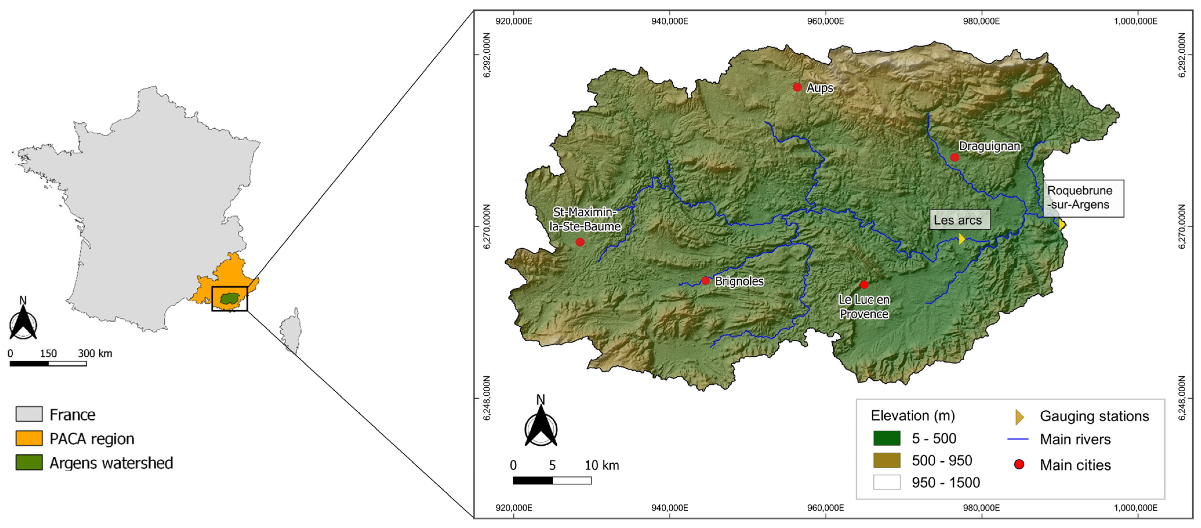
2.1. Study Area
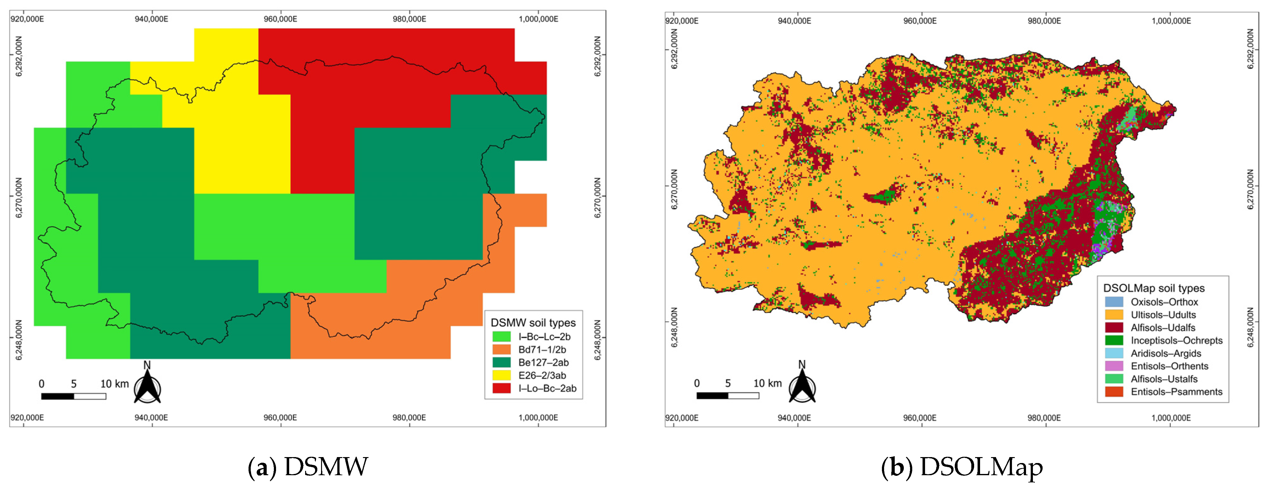
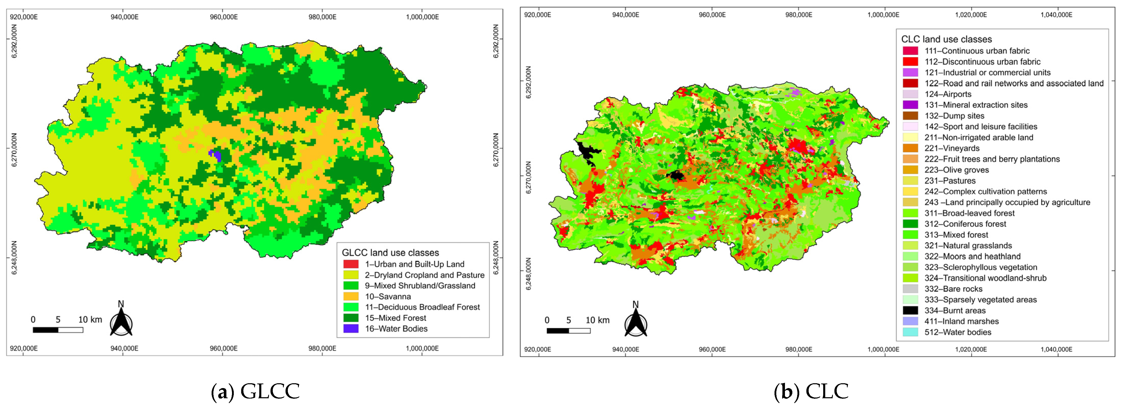
2.2. Input Datasets
2.3. SWAT Model
2.4. Soil and Land Use Datasets Translated into SWAT Hydrological Properties
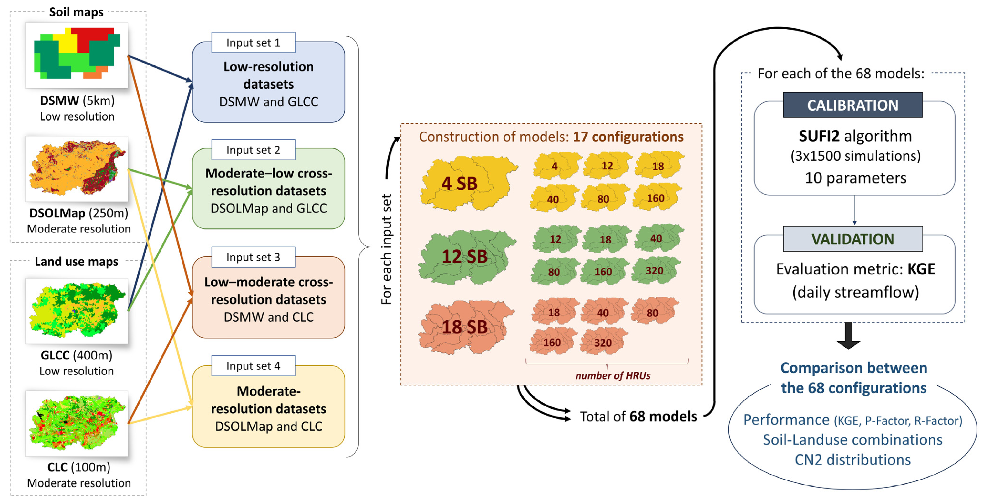
2.5. Model Experiments
2.6. Model Performance Evaluation
3. Results
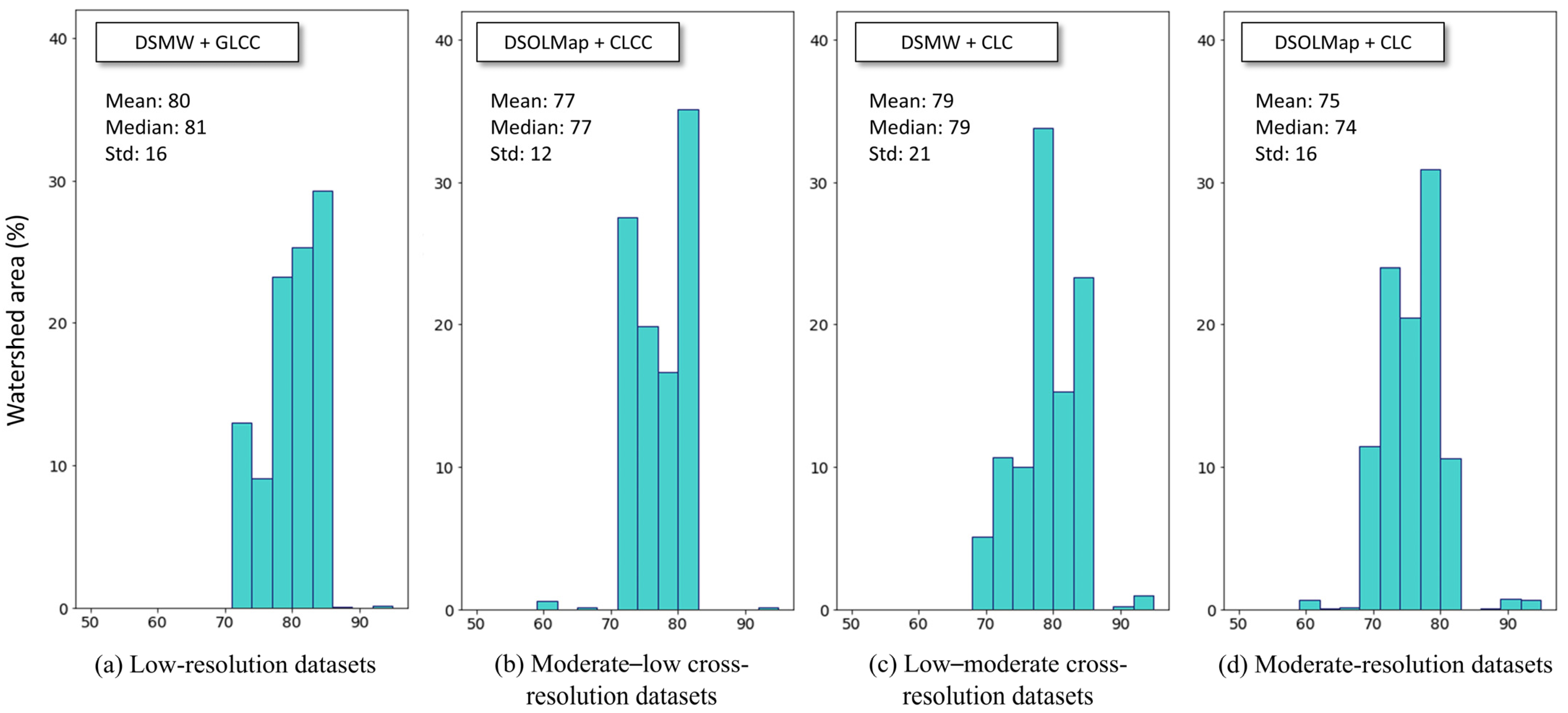
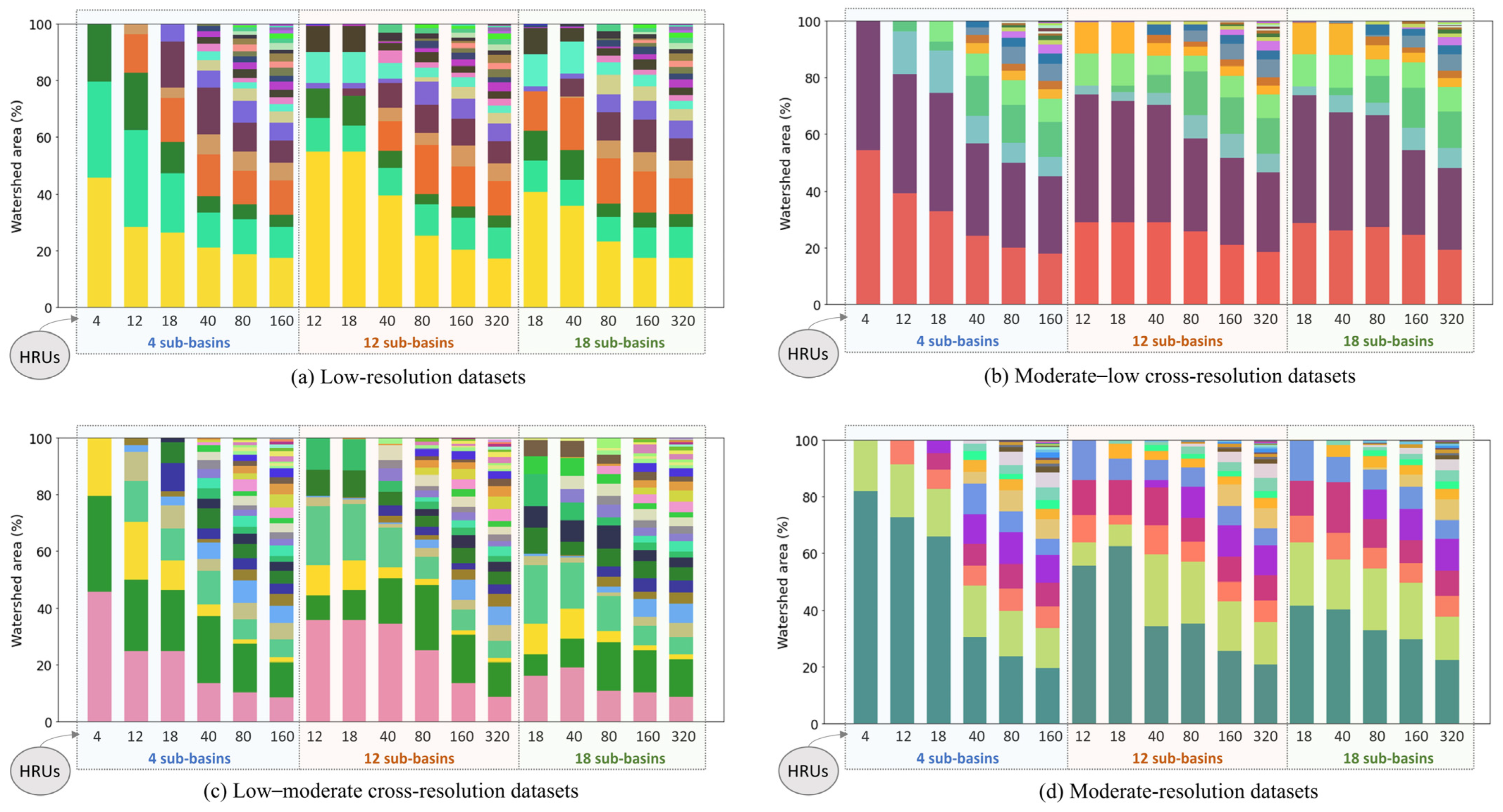
3.1. Comparison of Hydrological Properties from Soil and Land Use Datasets
3.2. Model Simulations
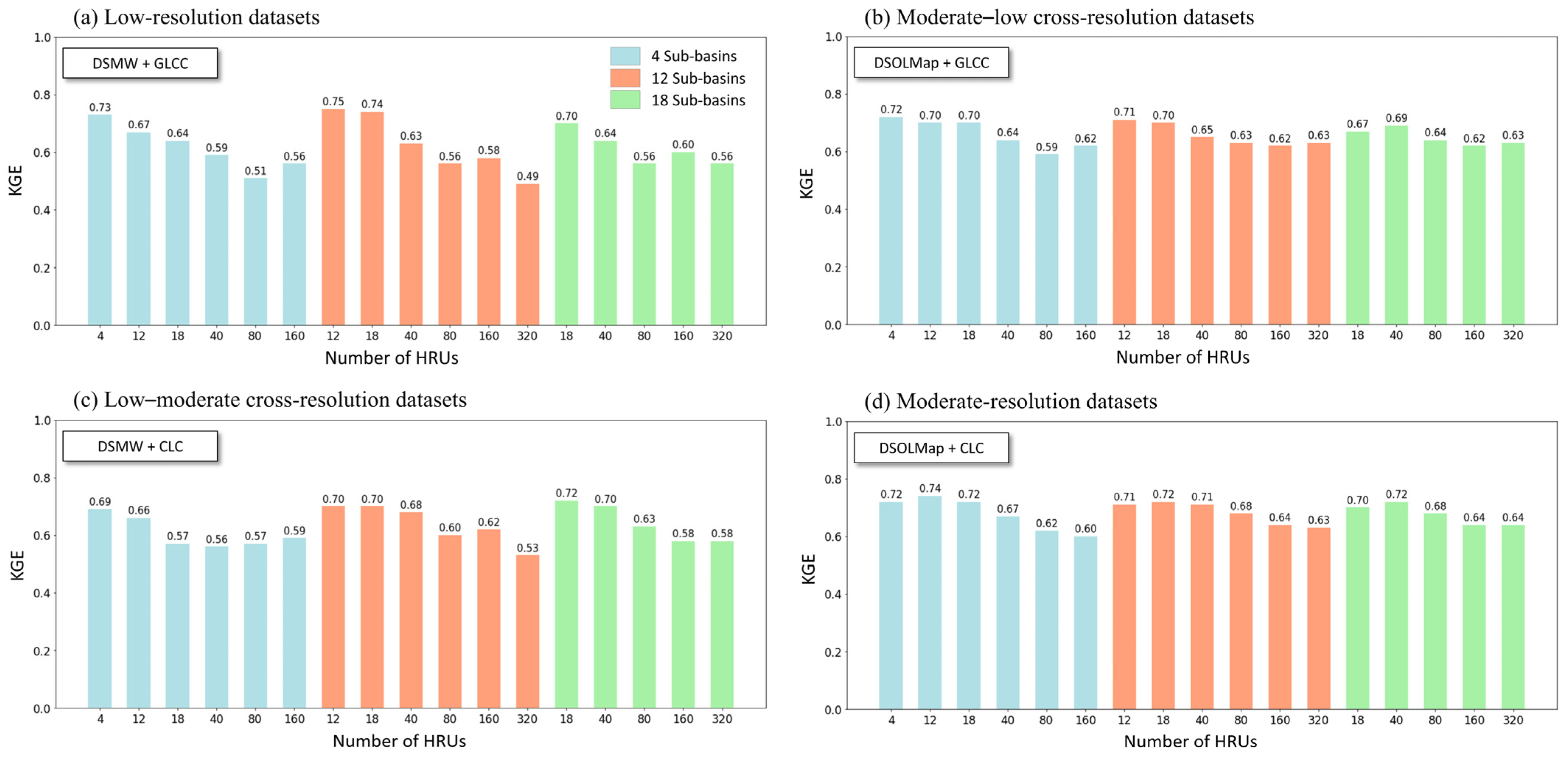
3.2.1. Performance Evolution with Increasing Discretization
3.2.2. Performance Evolution with Different Soil and Land Use Input Datasets
4. Discussion
4.1. Impact of Increasing Discretization on Model Performance
4.2. Impact of the Soil and Land Use Datasets on the Evolving Performance
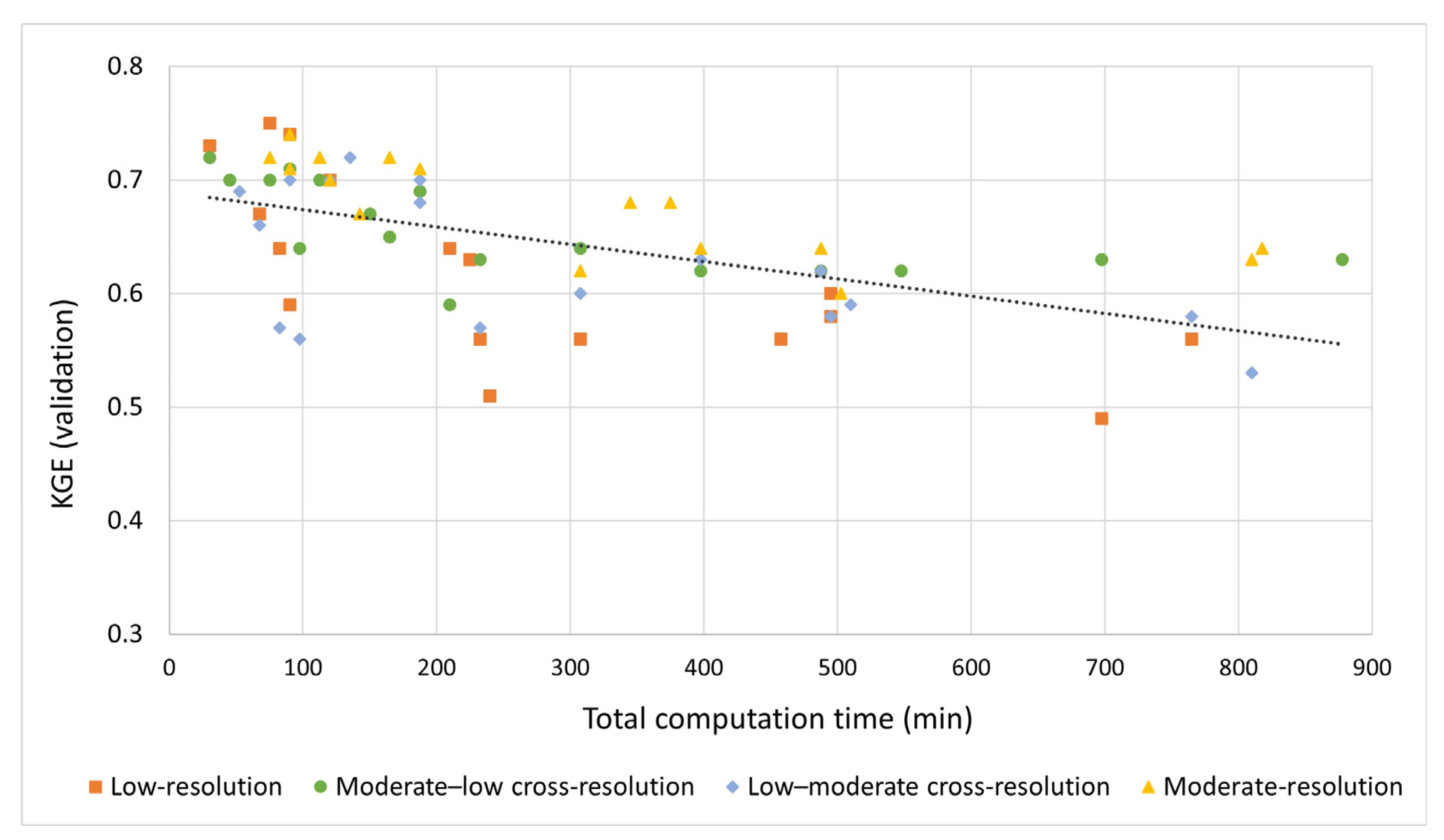
4.3. Optimal Discretization, Model Complexity, and Computation Time
4.4. Limitations and Future Work
5. Conclusions
- The performance of SWAT in simulating streamflow remains unaffected by the variation in the number of sub-basins. However, an increase in the number of HRUs results in a decrease in model performance, whatever the number of sub-basins or the input datasets.
- A higher sensitivity of the SWAT model to variations in the soil input is identified compared to changes in the land use dataset, with a faster decline in KGE performance with increasing discretization for the models based on the provided DSMW soil map than on the new DSOLMap. This sensitivity is attributed to the heterogeneity in soil types rather than to the spatial resolution of the inputs.
- Increasing discretization expands computation time and reduces model performance. It is therefore recommended to minimize the number of HRUs during watershed subdivision for optimal model accuracy of catchment-scale outputs.
Supplementary Materials
Author Contributions
Funding
Data Availability Statement
Conflicts of Interest
References
- Rajib, A.; Liu, Z.; Merwade, V.; Tavakoly, A.A.; Follum, M.L. Towards a Large-Scale Locally Relevant Flood Inundation Modeling Framework Using SWAT and LISFLOOD-FP. J. Hydrol. 2020, 581, 124406. [Google Scholar] [CrossRef]
- Kauffeldt, A.; Wetterhall, F.; Pappenberger, F.; Salamon, P.; Thielen, J. Technical Review of Large-Scale Hydrological Models for Implementation in Operational Flood Forecasting Schemes on Continental Level. Environ. Model. Softw. 2016, 75, 68–76. [Google Scholar] [CrossRef]
- Dash, S.S.; Sahoo, B.; Raghuwanshi, N.S. Improved Drought Monitoring in Teleconnection to the Climatic Escalations: A Hydrological Modeling Based Approach. Sci. Total Environ. 2023, 857, 159545. [Google Scholar] [CrossRef] [PubMed]
- Tran, T.-N.-D.; Tapas, M.R.; Do, S.K.; Etheridge, R.; Lakshmi, V. Investigating the Impacts of Climate Change on Hydroclimatic Extremes in the Tar-Pamlico River Basin, North Carolina. J. Environ. Manag. 2024, 363, 121375. [Google Scholar] [CrossRef]
- Hagemann, S.; Chen, C.; Clark, D.B.; Folwell, S.; Gosling, S.N.; Haddeland, I.; Hanasaki, N.; Heinke, J.; Ludwig, F.; Voss, F.; et al. Climate Change Impact on Available Water Resources Obtained Using Multiple Global Climate and Hydrology Models. Earth Syst. Dyn. 2013, 4, 129–144. [Google Scholar] [CrossRef]
- Tran, T.-N.-D.; Nguyen, B.Q.; Grodzka-Łukaszewska, M.; Sinicyn, G.; Lakshmi, V. The Role of Reservoirs under the Impacts of Climate Change on the Srepok River Basin, Central Highlands of Vietnam. Front. Environ. Sci. 2023, 11. [Google Scholar] [CrossRef]
- Jajarmizadeh, M.; Harun, S.; Salarpour, M. A Review on Theoretical Consideration and Types of Models in Hydrology. J. Environ. Sci. Technol. 2012, 5, 249–261. [Google Scholar] [CrossRef]
- Boyle, D.P.; Gupta, H.V.; Sorooshian, S. Toward Improved Calibration of Hydrologic Models: Combining the Strengths of Manual and Automatic Methods. Water Resour. Res. 2000, 36, 3663–3674. [Google Scholar] [CrossRef]
- Carpenter, T.M.; Georgakakos, K.P. Intercomparison of Lumped versus Distributed Hydrologic Model Ensemble Simulations on Operational Forecast Scales. J. Hydrol. 2006, 329, 174–185. [Google Scholar] [CrossRef]
- Refsgaard, J.C.; Knudsen, J. Operational Validation and Intercomparison of Different Types of Hydrological Models. Water Resour. Res. 1996, 32, 2189–2202. [Google Scholar] [CrossRef]
- Vilaseca, F.; Narbondo, S.; Chreties, C.; Castro, A.; Gorgoglione, A. A Comparison between Lumped and Distributed Hydrological Models for Daily Rainfall-Runoff Simulation. IOP Conf. Ser. Earth Environ. Sci. 2021, 958, 012016. [Google Scholar] [CrossRef]
- Savvidou, E.; Efstratiadis, A.; Koussis, A.D.; Koukouvinos, A.; Skarlatos, D. The Curve Number Concept as a Driver for Delineating Hydrological Response Units. Water 2018, 10, 194. [Google Scholar] [CrossRef]
- Arnold, J.G.; Srinivasan, R.; Muttiah, R.S.; Williams, J.R. Large Area Hydrologic Modeling and Assessment Part I: Model Development. J. Am. Water Resour. Assoc. 1998, 34, 73–89. [Google Scholar] [CrossRef]
- Neitsch, S.L.; Arnold, J.G.; Kiniry, J.R.; Williams, J.R. SWAT Theoretical Documentation—Version 2009; SWAT: College Station, TX, USA, 2011. [Google Scholar]
- Li, E.A.; Shanholtz, V.O.; Contractor, D.N.; Carr, J.C. Generating Rainfall Excess Based on Readily Determinable Soil and Landuse Characteristics. Trans. ASABE. 1977, 20, 1070–1078. [Google Scholar] [CrossRef]
- Zhong, K.; Chen, X.; Chen, Y.; Liu, M. Simulation of effects of topography and soil/land use spatial aggregation on sediment yield and runoff using AnnAGNPS. Trans. CSAE. 2016, 32, 127–135. [Google Scholar] [CrossRef]
- TAMU, (Texas A&M University) SWAT|Soil & Water Assessment Tool. 2024. Available online: https://swat.tamu.edu/ (accessed on 4 October 2023).
- FAO/UNESCO Digital Soil Map of the World. 2024. Available online: https://www.fao.org/soils-portal/soil-survey/soil-maps-and-databases/faounesco-soil-map-of-the-world/en/ (accessed on 31 July 2023).
- Dile, Y.; Srinivasan, R.; George, C. QGIS Interface for SWAT (QSWAT); SWAT: College Station, TX, USA, 2019. [Google Scholar]
- EROS Global Land Cover Characterization (GLCC). 2017. Available online: https://doi.org/10.5066/F7GB230D (accessed on 14 January 2025).
- Geza, M.; McCray, J.E. Effects of Soil Data Resolution on SWAT Model Stream Flow and Water Quality Predictions. J. Environ. Manage. 2008, 88, 393–406. [Google Scholar] [CrossRef]
- López-Ballesteros, A.; Nielsen, A.; Castellanos-Osorio, G.; Trolle, D.; Senent-Aparicio, J. DSOLMap, a Novel High-Resolution Global Digital Soil Property Map for the SWAT + Model: Development and Hydrological Evaluation. Catena. 2023, 231, 107339. [Google Scholar] [CrossRef]
- Rivas-Tabares, D.; de Miguel, Á.; Willaarts, B.; Tarquis, A.M. Self-Organizing Map of Soil Properties in the Context of Hydrological Modeling. Appl. Math. Model. 2020, 88, 175–189. [Google Scholar] [CrossRef]
- Zhao, A. Effect of Different Soil Data on Hydrological Process Modeling in Weihe River Basin of Northwest China. Arab. J. Geosci. 2016, 9, 664. [Google Scholar] [CrossRef]
- Escamilla-Rivera, V.; Cortina-Villar, S.; Vaca, R.A.; Golicher, D.; Arellano-Monterrosas, J.; Honey-Rosés, J. Effects of Finer Scale Soil Survey and Land-Use Classification on SWAT Hydrological Modelling Accuracy in Data-Poor Study Areas. J. Water Resour. Prot. 2022, 14, 100–125. [Google Scholar] [CrossRef]
- Jin, X.; Jin, Y.; Yuan, D.; Mao, X. Effects of Land-Use Data Resolution on Hydrologic Modelling, a Case Study in the Upper Reach of the Heihe River, Northwest China. Ecol. Model. 2019, 404, 61–68. [Google Scholar] [CrossRef]
- Romanowicz, A.A.; Vanclooster, M.; Rounsevell, M.; La Junesse, I. Sensitivity of the SWAT Model to the Soil and Land Use Data Parametrisation: A Case Study in the Thyle Catchment, Belgium. Ecol. Modell. 2005, 187, 27–39. [Google Scholar] [CrossRef]
- Al-Khafaji, M.; Saeed, F.H.; Al-Ansari, N. The Interactive Impact of Land Cover and DEM Resolution on the Accuracy of Computed Streamflow Using the SWAT Model. Water Air Soil Pollut. 2020, 231, 416. [Google Scholar] [CrossRef]
- Bouslihim, Y.; Rochdi, A.; El Amrani Paaza, N.; Liuzzo, L. Understanding the Effects of Soil Data Quality on SWAT Model Performance and Hydrological Processes in Tamedroust Watershed (Morocco). J. Afr. Earth Sci. 2019, 160, 103616. [Google Scholar] [CrossRef]
- Huang, J.; Zhou, P.; Zhou, Z.; Huang, Y. Assessing the Influence of Land Use and Land Cover Datasets with Different Points in Time and Levels of Detail on Watershed Modeling in the North River Watershed, China. Int. J. Environ. Res. Public Health 2013, 10, 144–157. [Google Scholar] [CrossRef] [PubMed]
- Ngeang, L.; Tantanee, S.; Anlauf, R. Comparison of FAO and SOILGRID Data Application on Streamflow and Sus-Pended Sediment Study Using SWAT Model: A Case Study of Upper Yom Basin, Thailand. GMSARN Int. J. 2019, 13, 104–111. [Google Scholar]
- Xiao, J.; Wang, Y.; Sun, J.; Xie, S.; Huang, Y.; Wan, Z.; Meng, L.; Li, X.; Zhong, K. Effect of Soil Spatial Aggregation Caused by the Calculation Unit Division on Runoff and Sediment Load Simulation in the SWAT Model. J. Hydrol. 2023, 626, 130345. [Google Scholar] [CrossRef]
- Vema, V.K.; Sudheer, K.P. Towards Quick Parameter Estimation of Hydrological Models with Large Number of Computational Units. J. Hydrol. 2020, 587, 124983. [Google Scholar] [CrossRef]
- Her, Y.; Frankenberger, J.; Chaubey, I.; Srinivasan, R. Threshold Effects in HRU Definition of the Soil and Water Assessment Tool. Trans. ASABE. 2015, 58, 367–378. [Google Scholar] [CrossRef]
- Arabi, M.; Govindaraju, R.S.; Hantush, M.M.; Engel, B.A. Role of Watershed Subdivision on Modeling the Effectiveness of Best Management Practices with Swat1. J. Am. Water Resour. Assoc. 2006, 42, 513–528. [Google Scholar] [CrossRef]
- Bingner, R.; Garbrecht, J.; Arnold, J.; Srinivasan, R. Effect of Watershed Subdivision on Simulation Runoff and Fine Sediment Yield. Trans. ASAE. 1997, 40, 1329–1335. [Google Scholar] [CrossRef]
- FitzHugh, T.W.; Mackay, D.S. Impacts of Input Parameter Spatial Aggregation on an Agricultural Nonpoint Source Pollution Model. J. Hydrol. 2000, 236, 35–53. [Google Scholar] [CrossRef]
- Kumar, S.; Merwade, V. Impact of Watershed Subdivision and Soil Data Resolution on SWAT Model Calibration and Parameter Uncertainty. J. Am. Water Resour. Assoc. 2009, 45, 1179–1196. [Google Scholar] [CrossRef]
- Jha, M.; Gassman, P.W.; Secchi, S.; Gu, R.; Arnold, J. Effect of Watershed Subdivision on Swat Flow, Sediment, and Nutrient Predictions. JAWRA J. Am. Water Resour. Assoc. 2004, 40, 811–825. [Google Scholar] [CrossRef]
- Alsilibe, F.; Bene, K. Watershed Subdivision and Weather Input Effect on Streamflow Simulation Using SWAT Model. Pollack Period. 2021, 17, 88–93. [Google Scholar] [CrossRef]
- Auda, O.; Bouisson, S.; Bourgeois, N.; Decuq, E.; Grimoin, V.; Jiguet, M.; Lantenois, J.M.; Metge, J.; Pelissier, J.; Thévenot, A.; et al. Livret historique sur les crues du Bassin de l’Argens 2015. Available online: https://var.fr/documents/20142/110788/PAPI+le+livret+sur+les+crues+historiques.pdf/b4c0f5d4-5e52-f6ca-fdc1-b9aabba83482 (accessed on 25 November 2024).
- SMA Le Territoire|Syndicat Mixte de l’Argens. 2017. Available online: http://syndicatargens.fr/le-sma/le-territoire/ (accessed on 11 December 2023).
- EauRMC Etude d’évaluation Des Volumes Prélevables Globaux—Bassin Versant de l’Argens (Phases 1, 2 et 3). 2013. Available online: https://www.rhone-mediterranee.eaufrance.fr/l-argens (accessed on 25 November 2024).
- NASA. Shuttle Radar Topography Mission (SRTM) Global; NASA: Washington, DC, USA, 2013.
- WateriTech WateriTech. Official Home Page. Available online: https://www.wateritech.com/resources (accessed on 22 November 2024).
- Büttner, G.; Kosztra, B.; Maucha, G.; Pataki, R.; Kleeschulte, S.; Hazeu, G.; Vittek, M.; Schröder, C.; Littkopf, A. Copernicus Land Monitoring Service Copernicus Land Monitoring Service—CORINE Land Cover User Manual; European Environment Agency: Copenhagen, Denmark, 2021. [Google Scholar]
- Muñoz-Sabater, J.; Dutra, E.; Agustí-Panareda, A.; Albergel, C.; Arduini, G.; Balsamo, G.; Boussetta, S.; Choulga, M.; Harrigan, S.; Hersbach, H.; et al. ERA5-Land: A State-of-the-Art Global Reanalysis Dataset for Land Applications. Earth Syst. Sci. Data. 2021, 13, 4349–4383. [Google Scholar] [CrossRef]
- SCHAPI, HydroPortail. Official Home Page. Available online: https://www.hydro.eaufrance.fr/ (accessed on 22 November 2024).
- Srinivasan, R.; Ramanarayanan, T.S.; Arnold, J.G.; Bednarz, S.T. Large Area Hydrologic Modeling and Assessment Part II: Model Application. J. Am. Water Resour. Assoc. 1998, 34, 91–101. [Google Scholar] [CrossRef]
- Haro-Monteagudo, D.; Palazón, L.; Beguería, S. Long-Term Sustainability of Large Water Resource Systems under Climate Change: A Cascade Modeling Approach. J. Hydrol. 2020, 582, 124546. [Google Scholar] [CrossRef]
- Krysanova, V.; White, M. Advances in Water Resources Assessment with SWAT—An Overview. Hydrol. Sci. J. 2015, 60, 771–783. [Google Scholar] [CrossRef]
- Moghadam, S.H.; Ashofteh, P.-S.; Singh, V.P. Sensitivity Analysis of Streamflow Parameters with SWAT Calibrated by NCEP CFSR and Future Runoff Assessment with Developed Monte Carlo Model. Theor Appl Clim. 2024, 155, 8797–8813. [Google Scholar] [CrossRef]
- Ougahi, J.H.; Karim, S.; Mahmood, S.A. Application of the SWAT Model to Assess Climate and Land Use/Cover Change Impacts on Water Balance Components of the Kabul River Basin, Afghanistan. J. Water Clim. Change 2022, 13, 3977–3999. [Google Scholar] [CrossRef]
- Moghadam, S.H.; Ashofteh, P.-S.; Loáiciga, H.A. Investigating the Performance of Data Mining, Lumped, and Distributed Models in Runoff Projected under Climate Change. J. Hydrol. 2023, 617, 128992. [Google Scholar] [CrossRef]
- Dwivedi, S.; Kothari, M.; Singh, P.K.; Chhipa, B.G.; Gupta, T. SWAT Model Applications in Hydrology: A Systematic Review. Int. J. Adv. Biochem. Res. 2024, 8, 603–607. [Google Scholar] [CrossRef]
- Darwiche-Criado, N.; Comín, F.A.; Masip, A.; García, M.; Eismann, S.G.; Sorando, R. Effects of Wetland Restoration on Nitrate Removal in an Irrigated Agricultural Area: The Role of in-Stream and off-Stream Wetlands. Ecol. Eng. 2017, 103, 426–435. [Google Scholar] [CrossRef]
- CARD SWAT Literature Database for Peer-Reviewed Journal Articles. 2023. Available online: https://www.card.iastate.edu/swat_articles/ (accessed on 1 October 2023).
- Tan, M.L.; Gassman, P.W.; Yang, X.; Haywood, J. A Review of SWAT Applications, Performance and Future Needs for Simulation of Hydro-Climatic Extremes. Adv. Water Resour. 2020, 143, 103662. [Google Scholar] [CrossRef]
- Nguyen, T.V.; Dietrich, J.; Dang, T.D.; Tran, D.A.; Van Doan, B.; Sarrazin, F.J.; Abbaspour, K.; Srinivasan, R. An Interactive Graphical Interface Tool for Parameter Calibration, Sensitivity Analysis, Uncertainty Analysis, and Visualization for the Soil and Water Assessment Tool. Environ. Modell. Software. 2022, 156, 105497. [Google Scholar] [CrossRef]
- Abbaspour, K.C.; Johnson, C.A.; van Genuchten, M.T. Estimating Uncertain Flow and Transport Parameters Using a Sequential Uncertainty Fitting Procedure. J. Hydrol. 2004, 3, 1340–1352. [Google Scholar] [CrossRef]
- Gupta, H.V.; Kling, H.; Yilmaz, K.K.; Martinez, G.F. Decomposition of the Mean Squared Error and NSE Performance Criteria: Implications for Improving Hydrological Modelling. J. Hydrol. 2009, 377, 80–91. [Google Scholar] [CrossRef]
- Moriasi, D.N. Hydrologic and Water Quality Models: Performance Measures and Evaluation Criteria. Trans. ASABE. 2015, 58, 1763–1785. [Google Scholar] [CrossRef]
- Knoben, W.J.M.; Freer, J.E.; Woods, R.A. Technical Note: Inherent Benchmark or Not? Comparing Nash–Sutcliffe and Kling–Gupta Efficiency Scores. Hydrol. Earth Syst. Sci. 2019, 23, 4323–4331. [Google Scholar] [CrossRef]
- Barbarosa, J.; Fernandes, A.; Lima, A.; Assis, L. The Influence of Spatial Discretization on HEC-HMS Modelling: A Case Study. J. Hydrol. 2019, 3, 442–449. [Google Scholar] [CrossRef]
- Githui, F.; Thayalakumaran, T. The Effect of Discretization of Hydrologic Response Units on the Performance of SWAT Model in Simulating Flow and Evapotranspiration. In Proceedings of the 19th International Congress on Modelling and Simulation—Sustaining Our Future: Understanding and Living with Uncertainty, Perth, Australia, 12–16 December 2011; pp. 3412–3418. [Google Scholar] [CrossRef]
- Gong, Y.; Shen, Z.; Liu, R.; Wang, X.; Chen, T. Effect of Watershed Subdivision on SWAT Modeling with Consideration of Parameter Uncertainty. J. Hydrol. Eng. 2010, 15, 1070–1074. [Google Scholar] [CrossRef]
- Zhou, S.; Wang, Y.; Guo, A.; Li, Z.; Chang, J.; Meng, D. Impacts of Changes in the Watershed Partitioning Level and Optimization Algorithm on Runoff Simulation: Decomposition of Uncertainties. Stoch. Environ. Res. Risk Assess. 2020, 34, 1909–1923. [Google Scholar] [CrossRef]
- Bhatta, B.; Shrestha, S.; Shrestha, P.K.; Talchabhadel, R. Evaluation and Application of a SWAT Model to Assess the Climate Change Impact on the Hydrology of the Himalayan River Basin. Catena. 2019, 181, 104082. [Google Scholar] [CrossRef]
- Tuo, Y.; Duan, Z.; Disse, M.; Chiogna, G. Evaluation of Precipitation Input for SWAT Modeling in Alpine Catchment: A Case Study in the Adige River Basin (Italy). Sci. Total Environ. 2016, 573, 66–82. [Google Scholar] [CrossRef]
- Veettil, A.V.; Mishra, A.K. Water Security Assessment Using Blue and Green Water Footprint Concepts. J. Hydrol. 2016, 542, 589–602. [Google Scholar] [CrossRef]
- Abbaspour, K.C.; Vaghefi, S.A.; Srinivasan, R. A Guideline for Successful Calibration and Uncertainty Analysis for Soil and Water Assessment: A Review of Papers from the 2016 International SWAT Conference. Water. 2018, 10, 6. [Google Scholar] [CrossRef]
- Whittaker, G.; Confesor, R., Jr.; Luzio, M.D.; Arnold, J.G. Detection of Overparameterization and Overfitting in an Automatic Calibration of SWAT. Trans. ASABE. 2010, 53, 1487–1499. [Google Scholar] [CrossRef]
- Abbaspour, K.C.; Rouholahnejad, E.; Vaghefi, S.; Srinivasan, R.; Yang, H.; Kløve, B. A Continental-Scale Hydrology and Water Quality Model for Europe: Calibration and Uncertainty of a High-Resolution Large-Scale SWAT Model. J. Hydrol. 2015, 524, 733–752. [Google Scholar] [CrossRef]
- Kamali, B.; Abbaspour, K.C.; Yang, H. Assessing the Uncertainty of Multiple Input Datasets in the Prediction of Water Resource Components. Water. 2017, 9, 709. [Google Scholar] [CrossRef]
- Busico, G.; Colombani, N.; Fronzi, D.; Pellegrini, M.; Tazioli, A.; Mastrocicco, M. Evaluating SWAT Model Performance, Considering Different Soils Data Input, to Quantify Actual and Future Runoff Susceptibility in a Highly Urbanized Basin. J. Environ. Manage. 2020, 266, 110625. [Google Scholar] [CrossRef]
- El-Sadek, A.; İRvem, A. Evaluating the Impact of Land Use Uncertainty on the Simulated Streamflow and Sediment Yield of the Seyhan River Basin Using the SWAT Model. Turk. J. Agric. For. 2014, 38, 515–530. [Google Scholar] [CrossRef]
- Wu, L.; Xu, Y.; Li, R. Effects of Input Data Accuracy, Catchment Threshold Areas and Calibration Algorithms on Model Uncertainty Reduction. Eur. J. Soil Sci. 2024, 75, e13519. [Google Scholar] [CrossRef]
- Tolson, B.A.; Shoemaker, C.A. Dynamically Dimensioned Search Algorithm for Computationally Efficient Watershed Model Calibration. Water Resour. Res. 2007, 43. [Google Scholar] [CrossRef]
- Zamani, M.; Shrestha, N.K.; Akhtar, T.; Boston, T.; Daggupati, P. Advancing Model Calibration and Uncertainty Analysis of SWAT Models Using Cloud Computing Infrastructure: LCC-SWAT. J. Hydroinf. 2020, 23, 1–15. [Google Scholar] [CrossRef]
- Abbaspour, K.C.; Yang, J.; Maximov, I.; Siber, R.; Bogner, K.; Mieleitner, J.; Zobrist, J.; Srinivasan, R. Modelling Hydrology and Water Quality in the Pre-Alpine/Alpine Thur Watershed Using SWAT. J. Hydrol. 2007, 333, 413–430. [Google Scholar] [CrossRef]
- Tapas, M.R.; Etheridge, R.; Tran, T.-N.-D.; Le, M.-H.; Hinckley, B.; Nguyen, V.T.; Lakshmi, V. Evaluating Combinations of Rainfall Datasets and Optimization Techniques for Improved Hydrological Predictions Using the SWAT+ model. J. Hydrol. Reg. Stud. 2025, 57, 102134. [Google Scholar] [CrossRef]


| Group | Parameter | Description | Default Value | Range | Change |
|---|---|---|---|---|---|
| Infiltration | CN2 | SCS curve number | Soil data | [−0.25, 0.25] | Relative |
| Soil | SOL_AWC | Available water capacity | Soil data | [−0.25, 0.25] | Relative |
| Evaporation | ESCO | Soil evaporation compensation factor | 0.95 | [0, 1] | Replace |
| Groundwater | GWQMN | Threshold water depth in the shallow aquifer for return flow to occur (m) | 0 | [0, 5000] | Replace |
| Groundwater | GW_REVAP | Groundwater revap coefficient | 0.02 | [0.02, 0.2] | Replace |
| Groundwater | REVAPMN | Threshold water depth in the shallow aquifer for revap or percolation to the deep aquifer to occur (mm) | 1 | [0, 750] | Replace |
| Groundwater | ALPHA_BF | Baseflow alpha factor | 0.048 | [0.01, 1] | Replace |
| Groundwater | GW_DELAY | Groundwater delay time (days) | 31 | [0, 500] | Replace |
| Groundwater | RCHRG_DP | Deep aquifer percolation fraction | 0.05 | [0.01, 0.99] | Replace |
| Soil | DEP_IMP | Depth to impervious layer in soil profile | 0.5 | [−0.25, 0.25] | Relative |
| Mean Clay (%) | Mean Silt (%) | Mean Sand (%) | |
|---|---|---|---|
| DSMW | 28 | 34 | 38 |
| DSOLMap | 23 | 32 | 45 |
| Difference | 5 | 2 | 7 |
| (a) From GLCC classes | ||||
| Area (%) | CN2C | CN2D | ||
| 35.2 | CRDY | Dryland, Cropland, and Pasture | 81 | 85.5 |
| 28.0 | FOMI | Mixed Forest | 73 | 79 |
| 16.7 | FODB | Deciduous Broadleaf Forest | 77 | 83 |
| 12.2 | SAVA | Savanna | 76.5 | 82 |
| 7.8 | MIGS | Mixed Shrubland/Grassland | 76.5 | 82 |
| Weighted average CN2 | ——— | 77 | 82.5 | |
| (b) From CLC classes | ||||
| Area (%) | CN2C | CN2D | ||
| 24.4 | FRST (FOMI) | Forest—Mixed (Mixed Forest) | 73 | 79 |
| 17.2 | FODB | Deciduous Broadleaf Forest | 77 | 83 |
| 13.9 | SHRB | Shrubland | 74 | 80 |
| 11.6 | GRAP | Vineyard | 77 | 83 |
| 11.4 | FRSE | Forest—Evergreen | 70 | 77 |
| 10.6 | CRGR | CropLand/GrassLand mosaic | 81 | 85.5 |
| 6.5 | URLD | Residential—Low Density | 72 | 79 |
| 0.8 | OLIV | Olives | 77 | 83 |
| 0.8 | BARR | Barren | 91 | 94 |
| 0.6 | GRAS | Grassland | 79 | 84 |
| 0.6 | UIDU | Industrial | 72 | 79 |
| 0.5 | BSVG | Baren or Sparsely vegetated | 74 | 80 |
| 0.5 | ORCD | Orchard | 77 | 83 |
| 0.3 | UTRN | Transportation | 72 | 79 |
| 0.3 | PAST | Pasture | 79 | 84 |
| Weighted average CN2 | ——— | 75 | 81 | |
Disclaimer/Publisher’s Note: The statements, opinions and data contained in all publications are solely those of the individual author(s) and contributor(s) and not of MDPI and/or the editor(s). MDPI and/or the editor(s) disclaim responsibility for any injury to people or property resulting from any ideas, methods, instructions or products referred to in the content. |
© 2025 by the authors. Licensee MDPI, Basel, Switzerland. This article is an open access article distributed under the terms and conditions of the Creative Commons Attribution (CC BY) license (https://creativecommons.org/licenses/by/4.0/).
Share and Cite
Puche, M.; Troin, M.; Fox, D.; Royer-Gaspard, P. Optimizing Spatial Discretization According to Input Data in the Soil and Water Assessment Tool: A Case Study in a Coastal Mediterranean Watershed. Water 2025, 17, 239. https://doi.org/10.3390/w17020239
Puche M, Troin M, Fox D, Royer-Gaspard P. Optimizing Spatial Discretization According to Input Data in the Soil and Water Assessment Tool: A Case Study in a Coastal Mediterranean Watershed. Water. 2025; 17(2):239. https://doi.org/10.3390/w17020239
Chicago/Turabian StylePuche, Mathilde, Magali Troin, Dennis Fox, and Paul Royer-Gaspard. 2025. "Optimizing Spatial Discretization According to Input Data in the Soil and Water Assessment Tool: A Case Study in a Coastal Mediterranean Watershed" Water 17, no. 2: 239. https://doi.org/10.3390/w17020239
APA StylePuche, M., Troin, M., Fox, D., & Royer-Gaspard, P. (2025). Optimizing Spatial Discretization According to Input Data in the Soil and Water Assessment Tool: A Case Study in a Coastal Mediterranean Watershed. Water, 17(2), 239. https://doi.org/10.3390/w17020239