Evaluate Water Yield and Soil Conservation and Their Environmental Gradient Effects in Fujian Province in South China Based on InVEST and Geodetector Models

Abstract

Fujian Province is an important soil and water conservation region in hilly South China. However, there has been limited attention paid to the assessment of water production and soil conservation at the provincial level, and the distribution patterns of ecosystem services under different environmental gradients in hilly regions have not been revealed. This study evaluated the spatiotemporal characteristics of water yield and soil conservation based on the InVEST model in 2000, 2010, and 2020, and explored their differences under six environmental gradients: elevation, slope, terrain position index, geomorphy, LULC, and NDVI. The results and statistics of the InVEST model showed significant spatial differentiation and temporal change in water yield; the distribution and changes in water yield and soil conservation both exhibited obvious clustering characteristics of cold and hot spots (low and high values); and the differences in distribution and change in water yield in different cities were higher than those in soil conservation. The distribution index and Geodetector showed that there were spatiotemporal differences in distribution and change characteristics of water yield and soil retention in different environmental gradients; the distribution and change differences in water yield were generally lower than those of soil conservation and the degree of distribution and change in water yield and soil conservation were generally more sensitive to the response of terrain factors (slope, TPI, and DEM). The high-value important regions of water yield and soil conservation were 1000 to 2160 m for DEM, 25° to 70.2° for slope, 0.81 to 1.42 for TPI, medium mountain for geomorphy, forest land for LULC, and 0.9 to 0.92 for NDVI, which indicates mountainous regions with high altitude, steep slopes, significant terrain changes, and high forest vegetation coverage. This study indicates that ecosystem services exhibit spatiotemporal differences in distributions across different environmental gradients, and attention should be paid to adapting to local conditions in ecological environment development.

1. Introduction

Ecosystem services (ESs) are the benefits that humans acquire from ecosystems, either directly or indirectly [1,2,3]. Land use and land cover (LULC) change are two of the key factors that drive changes in human activity and the natural environment [4,5,6,7]. Human activities have significantly affected ecosystem services, not only LULC change but also pollution, decreased biodiversity, and so on [8,9]. Therefore, evaluating ecosystem service functions is crucial for achieving sustainable development goals (SDGs), human well-being, and building a beautiful China.

According to the Millennium Ecosystem Assessment (MEA), there are four types of ecosystem services: provisioning services, supporting services, regulating services, and cultural services [10]. Among them, water yield and soil conservation are important ecosystem services, whether in arid or humid areas [11,12,13], as they provide one of the important foundations for maintaining ecosystem stability and biodiversity. There are multiple models available for quantitatively evaluating ecosystem services, including the Integrated Valuation of Ecosystem Services and Tradeoffs (InVEST) model [14,15], the Social Values for Ecosystem Services (SoLVES) model [16,17], and the Artificial Intelligence for Ecosystem Services (ARIES) model [18,19]. Of these, the application and development of the InVEST model have promoted the development of ecosystem services evaluation research towards quantification, spatialization, and visualization. This has made the application research of the InVEST model more in-depth and widespread around the world [20,21,22,23,24].

South China is mainly mountainous and hilly, with abundant monsoon precipitation, dense river networks, and widely distributed subtropical vegetation [25,26,27]. However, the spatiotemporal variation in water resources here is significant due to the unstable monsoon precipitation. A study from the Sancha River in southwestern China showed that the water yield in the basin increased from 1990 to 2010, and climate change contributed the majority of the water yield changes, far exceeding the LULC changes, indicating that the grain-for-green program of China had a negative impact on water yield [28]. In addition, during this period, the water yield in karst mountainous areas showed a fluctuating decreasing trend, but in the economic development scenario, the water yield in 2030 slightly increased compared to the actual water yield in 2010 [29]. Similarly, studies in different regions of South China, such as the Hunan and Jiangxi provinces, have shown that the impact of climate change on water yield was higher than that of LULC changes, especially with reference to evapotranspiration and parameter Z value of seasonal climate factors, and water yield will increase under climate change scenarios in the future [12,13,30,31,32]. However, the spatial pattern of watershed water yield services was also susceptible to LULC changes [31], and different forest types and landscape patterns can also affect the spatial pattern of water yield services [33,34]. Even research in Jiangxi Province has found that land use is the main driving factor for the spatial differentiation of water production services, and it has a negative impact [35]. At the same time, South China is also facing a wide range of soil conservation tasks, with the significant erosion of the surface by rainwater. Coupled with the long history of human development, damage to the surface environment has led to intensified soil erosion. As one of the eight major tributaries of the Yangtze River, soil erosion in the Ganjiang River Basin showed a trend of first decreasing and then increasing from 2000 to 2020; erosion intensity and sediment transport rate (SDR) decreased due to the influence of engineering measures such as reservoirs; and precipitation was found to be the main factor affecting soil erosion, inhibiting the mitigating effect of high vegetation coverage on soil erosion [36]. It has also been observed that there are spatial differences in soil erosion in the Liaohe River Basin of Jiangxi, with an increasing trend from flat and well-covered areas to sparsely vegetated mountainous areas [37]. In addition, using structural equation modeling, it was found that economic development was the main controlling factor for soil erosion in Jiangxi Province, and agricultural output was the main promoting factor for soil erosion [38]. In the northern part of Guangdong Province, there are also differences in rainfall erosivity caused by changes in precipitation, leading to changes in soil erosion, and it was found that the main factors for differences in soil retention space were land use type, altitude, and slope [39]. Chongqing, in southwestern China, has relatively obvious terrain undulations, and studies have shown that soil erosion was more severe in low mountain and hilly areas, with only slight erosion in areas with gentle slopes [40]. The study on the driving forces of soil erosion in the Huaihe River Basin also indicates that the changes in soil erosion and soil conservation were mainly influenced by slope and rainfall, and the steepness and length of slope were the biggest factors affecting soil erosion [41]. The InVEST model provides great convenience for quantifying ecosystem services, and these extensive related studies have enriched the exploration of ecosystem services at different temporal and spatial scales, especially in South China, which is also the focus of this study. Considering the differences in background conditions among different research areas, there may be spatial heterogeneity in the spatiotemporal distribution of ecosystem services. Therefore, it is necessary to consider the environmental gradient effect of ecosystem services. However, existing research has not considered this aspect, and this study fills this gap in the environmental gradient effects of ecosystem services.

Fujian Province is located in South China, and in the secondary regionalization south Yangtze River hilly subregion, based on the regionalization of soil and water conservation in China [42,43]. Changting County, located in the western Fujian Province, is a typical red soil erosion area in southern China. It has strong rainfall erosion, severe terrain undulations, porous soil, sparse vegetation, and excessive human activities, resulting in severe soil erosion and fragility on a large scale, so more than 50% of the area is susceptible to soil erosion [44]. Researchers and engineers have used various methods, such as simulation, sampling, and investigation, to analyze soil erosion and surface runoff under large-scale infrastructure construction conditions [45], the soil and water conservation effects of ecological restoration projects [46], flood runoff and sediment characteristics after treatment [47], the relationship between erosion intensity and soil erosion evolution [48], and the impact of agricultural land consolidation and farmer behavior on soil and water conservation services [49,50]. These measured and surveyed data are important supporting resources for soil and water conservation. However, there is relatively little research on ecosystem services evaluation at the provincial level in Fujian Province, especially focusing on analyzing water yield and soil conservation services, as well as ecosystem services evaluation without environmental gradients research. The aim of this study is to apply the InVEST model to evaluate important ecosystem services (water yield and soil conservation) in Fujian Province, and quantify their environmental gradient effects, including elevation, slope, terrain position index, geomorphy, LULC, and NDVI. This study will help supplement research on ecosystem service assessment and act as a reference material for the sustainable development of ecology and the optimization of land space in Fujian Province.

2. Materials and Methods

2.1. Study Area

Fujian Province (23°30′ N to 28°20′ N; 115°50′ E to 120°45′ E) is located on the southeast coast of China (Figure 1a), facing the Taiwan Strait to the east, with an area of about 12.4 × 10⁴ km². There are a total of 9 cities in Fujian Province, with Fuzhou being the provincial capital and Xiamen having a relatively high level of economic development (Figure 1b). Fujian Province has an altitude of about 0 m to 2160 m, mainly consisting of low mountains and hills, accounting for more than 80% of the province’s area. Fujian Province is located in the subtropical monsoon climate zone and is influenced by the East Asian summer monsoon and East Asian winter monsoon [51,52], and has a warm and humid climate. The average annual temperature in Fujian Province is about 17 °C to 20 °C, with the average temperature in the coldest month (Jan to Feb) being about 6 °C to 10 °C, and the average temperature in the hottest month (July to Aug) being about 33 °C to 37 °C. The average annual hours of sunshine are 1700 h to 2000 h, and the average annual precipitation in most areas is 1000 mm to 2000 mm. Benefitting from the hilly terrain and abundant hydrothermal conditions, Fujian Province has the best vegetation coverage in China, with only the eastern coastal areas having poor vegetation coverage. Also, due to the abundant monsoon precipitation and undulating terrain, this area faces severe water and soil conservation tasks. Related studies indicate that the increase in erosion associated with the replacement of native vegetation with bare ground or grasses due to large-scale infrastructure projects in Fujian from 1999 to 2004 amounted to an estimated loss of 1.76 × 10⁷ tonnes of top-soil and 3.04 × 10⁸ m³ of surface runoff from the province during the bare soil construction phase [45]. The degree of soil erosion vulnerability gradually decreased from 1999 to 2015 in the middle of the Zhuxi watershed in Fujian, and low levels of vulnerability were distributed from fragmentation to concentrated distribution, while high levels of vulnerability presented the opposite trend [53].

2.2. Research Framework and Data

There are three stages to achieving the evaluation objectives of ecosystem services in Fujian Province in this study (Figure 2): (1) evaluate water yield and soil conservation based on the InVEST model; (2) analyze the distribution characteristics of water yield and soil conservation at different levels of environmental gradients of elevation, slope, terrain position index, geomorphy, LULC, and NDVI; and (3) explore the driving factors of spatial differentiation and change in water yield and soil conservation based on the Geodetector model.

Three years of data (2000, 2010, and 2020) on land use/land cover (LULC) were obtained from the National Earth System Science Data Center (http://www.geodata.cn/). The LULC data consist of 6 primary classifications and 23 subcategories and are a part of the China Multi-Period Land Use and Land Cover Remote Sensing Monitoring Dataset (CNLUCC). The LULC data use Landsat remote sensing images from the United States as their main information source, and a national scale multi-period land use/land cover thematic database in China was constructed through manual visual interpretation [6,54,55]. Annual precipitation data were obtained from the China Meteorological Data Service Center (https://data.cma.cn/). Average annual potential evapotranspiration data were obtained from Global Aridity Index and Potential Evapotranspiration Climate (Global-AI_PET) Database v3 (https://csidotinfo.wordpress.com/) [56]. Soil attribute data were obtained from Harmonized World Soil Database v 1.2 (HWSD, https://www.fao.org/soils-portal/data-hub/soil-maps-and-databases/harmonized-world-soil-database-v12/en/ (accessed on 20 March 2024)). Available water capacity data were obtained from SoilGrids250m (https://data.isric.org/geonetwork/srv/eng/catalog.search#/metadata/e33e75c0-d9ab-46b5-a915-cb344345099c (accessed on 21 March 2024)) [57]. Elevation data were obtained from the Shuttle Radar Topography Mission (SRTM, https://earthdata.nasa.gov/). Geomorphic data were obtained from Spatial Distribution Data of 1 million Geomorphical Types in China from the Resource and Environmental Science Data Center of the Chinese Academy of Sciences (RESDC-CAS, https://www.resdc.cn/). The NDVI data are a part of the China Annual Normalized Difference Vegetation Index (CNDVI) Spatial Distribution Dataset from RESDC-CAS [58]. All data use a 1 km × 1 km spatial resolution.

2.3. Water Yield Evaluation Based on the InVEST Model

2.3.1. Evaluation Principles of Water Yield

The water yield (WY) evaluation in the InVEST model is based on the water balance method, and comprehensively considers the effects of soil texture, soil structure, precipitation characteristics, solar radiation evaporation, surface transpiration, land use types, topography, water resources confluence, etc., which are calculated by the following equations [12,59,60]:

$$Y_{xj}=\left(1-{\displaystyle \frac{{AET}_{xj}}{P_x}}\right)\times P_x$$

(1)

$${\displaystyle \frac{{AET}_{xj}}{P_x}}={\displaystyle \frac{1+{\omega }_x{R}_{xj}}{1+{\omega }_x{R}_{xj}+1/R_{xj}}}$$

(2)

$${\omega }_x=Z\times {\displaystyle \frac{{AWC}_x}{P_x}}+1.25$$

(3)

$$R_{xj}={\displaystyle \frac{{k\times ET}_0}{P_x}}$$

(4)

$${AWC}_x=Min\left({RLD}_x,{RD}_x\right)\times {PAWC}_x$$

(5)

$$\begin{gathered} {PAWC}_x=54.509-0.132\times Sand-0.03\times {Sand}^2-0.55\times Silt-0.006\times {Silt}^2-0.738\times Clay \\ +0.007\times {Clay}^2-2.688\times C+0.501\times C^2 \end{gathered}$$

(6)

In Equation (1), Y_xj is the average annual water yield (mm) of the jth land use in raster cell x; AET_xj is the actual annual evapo-transpiration (mm) of the jth land use; and P_x is average annual precipitation. AET_xj/P_x is based on the Budyko curve [61], calculated from Equation (2). ω_x is a non-physical parameter of natural climate–soil properties, calculated from Equation (3). Z (Zhang) is an empirical coefficient, which can represent the regional precipitation distribution and hydrogeological characteristics [61]. In this study, the default 5 were used, and referring to the land use and precipitation in 2010, the water yield (994.6 mm) is close to the annual water resources (about 1000 mm). AWC_x is the effective soil water content (mm), determined by soil texture and effective soil depth when the model requires the proportional parameter (plant available water fraction) and is calculated from Equation (5), while also referring to available water capacity from SoilGrids250m [57]. The ω_x base parameter is 1.25, which represents the ratio of annual water demand to annual precipitation for vegetation in bare ground (root depth of 0) [62]. In Equation (4), R_xj is the dryness index of the jth land use type, which is the ratio of evapotranspiration to precipitation; ET₀ is the potential evapotranspiration (mm/a); and k is the evapotranspiration coefficient, which is obtained from the vegetation leaf area index and can also be determined by the vegetation nature of LULC [63]. In Equation (5), RLD_x and RD_x are restricted layer depth and root depth, respectively. In Equation (6), PWAC_x is plant available water fraction; Sand, Silt, Clay, and C are the soil sand, silt, clay and organic carbon contents, respectively.

2.3.2. Input Data for Water Yield Evaluation

According to the annual water production module of the InVEST model, 8 parameters are required. (1) Precipitation data, i.e., the measured results of precipitation data for the years 2000, 2010, and 2020, are provided in this study (Figure 3a–c). (2) Potential evapotranspiration data refers to the amount of water that may dissipate through soil evaporation and plant evapotranspiration under sufficient water conditions. Average annual potential evapotranspiration data from 1970 to 2000 are provided in this study (Figure 3d). (3) Root restriction depth refers to the maximum depth at which plant roots can extend in soil due to the different physical and chemical characteristics of the environment. In this study, root restriction depth is quantified through different LULC subcategory types (

Table 1. Root restriction depth based on LULC types.

ID	Name	Root Restriction Depth (mm)	ID	Name	Root Restriction Depth (mm)
1	Cultivated land	2000	11	Paddy field	2200
			12	Dry land	1800
2	Forest land	3000	21	Closed forest land	3500
			22	Shrubs forest land	3000
			23	Sparse forest land	2500
			24	Other forest land	2000
3	Grassland	2500	31	High-coverage grassland	2700
			32	Medium-coverage grassland	2500
			33	Low-coverage grassland	2200
4	Water body	1	41	Rivers and canals	1
			42	Lake	1
			43	Reservoir pits and ponds	1
			44	Glacier and snow land	1
			45	Mudflat	1
			46	Beach land	1
5	Built-up land	1	51	Urban land	1
			52	Rural residential areas	1
			53	Other construction land	1
6	Unused land	10	61	Sand	10
			62	Gobi	1
			63	Saline alkali land	10
			64	Swamp land	100
			65	Bare land	10
			66	Bare rocky terrain	1

, Figure 3e). (4) Plant available water content (PAWC) refers to the proportion of water provided by soil layers for plant growth. This study uses soil attribute data to calculate the PAWC, also referring to available water capacity from SoilGrids250m [57] (Figure 3f). (5) For LULC, this study provides primary category data for the years 2000, 2010, and 2020 (Figure 3g–i). (6) Biophysical table represents the biophysical coefficient data corresponding to LULC, which mainly encompasses the attributes of each land use type rather than the grid unit attributes in the grid map [59]. This table needs to be adjusted according to the study area (

Table 2. Biophysical table of LULC for water yield and soil conservation evaluation.

Code	Description	Water Yield			Soil Conservation
		Vegetation	Root Depth (mm)	Kc	usle_c	usle_p
1	Cultivated land	1	2000	0.9	0.412	1
2	Forest land	1	3000	1	0.025	1
3	Grassland	1	2500	0.75	0.034	1
4	Water body	0	1	1.2	0	1
5	Built-up land	0	1	0.1	0.99	1
6	Unused land	0	10	0.15	1	1

). (7) The Z parameter, i.e., the seasonal constant Z, is a floating value defined based on the distribution of seasonal precipitation, sorted from 1 to 30. With reference to relevant research and debugging, this value was determined to be 5 in this study. (8) Watersheds encompassed the overall study area.

2.4. Soil Conservation Evaluation Based on the InVEST Model

2.4.1. Evaluation Principles of Soil Conservation

Soil conservation (SC) evaluation in the InVEST model is based on the universal soil loss equation (USLE) calculation method based on pixel scale and uses the sediment delivery ratio module to calculate the total or average soil conservation at the watershed scale [41,64,65]. The soil conservation of ecosystems includes two parts, namely erosion reduction and sediment retention, which are expressed as the difference between potential erosion and actual erosion, and the product of sediment inflow and sediment retention efficiency. The calculation method is as follows [41,64,65]:

$${SEDRET}_x=R_x\times K_x\times {LS}_x\times \left(1-C_x\times P_x\right)+{SEDR}_x$$

(7)

$${SEDR}_x={SE}_x\sum _{y=1}^{x-1}{USLE}_y\prod _{z=y+1}^{x-1}\left(1-{SE}_z\right)$$

(8)

$${USLE}_x=R_x\times K_x\times {LS}_x\times C_x\times P_x$$

(9)

$$R_x=\sum _{i=1}^{12}\left(-1.5527+0.1792P_i\right)\times 17.02$$

(10)

$$K_x=\begin{array}{c}\left[0.2+0.3e^{-0.0256S_a\left(1-{\displaystyle \frac{S_i}{100}}\right)}\right]\times {\left[{\displaystyle \frac{S_i}{\left(S_c+S_i\right)}}\right]}^{0.3}\times \left(1-{\displaystyle \frac{0.25C}{C+e^{3.72-2.95C}}}\right)\\ \times \left[1-0.7\left(1-{\displaystyle \frac{S_a}{100}}\right)\right]/\left[1-{\displaystyle \frac{S_a}{100}}+e^{-5.51+22.9\left(1-{\displaystyle \frac{S_a}{100}}\right)}\right]\times 0.1317\end{array}$$

(11)

In Equations (7)–(9), SEDRET_x and SEDR_x represent the soil retention and sediment retention of grid x, respectively; USLE_x and USLE_y represent the actual erosion of grid x and its uphill grid y; R_x, K_x, LS_x, C_x, and P_x represent the rainfall erosivity factor, soil erodibility factor, terrain factor, coverage management factor, and soil and water conservation measure factor of grid x, respectively; and SE_x represents the sediment retention efficiency of grid x. In Equation (10), P_i represents the rainfall in the i-th month, which is a calculation formula for the rainfall erosivity factor that is in line with the actual situation in Fujian Province [66]. In Equation (11), S_a represents the sand content; S_i represents the powder particle content; S_c represents the content of clay particles; and C represents the organic carbon content, and this formula is currently the most commonly used EPIC model for calculating soil erodibility factors. The calculation of LS adopts the default method of the InVEST model, and the value of LS is calculated in sections of gentle and steep slopes, and the default slope threshold is 25°; C_x and P_x refer to relevant research [41,64,65].

2.4.2. Input Data for Soil Conservation Evaluation

According to the sediment delivery ratio module of the InVEST model, 11 parameters are required. (1) Digital elevation model (DEM): a GIS raster dataset where each grid unit corresponds to an elevation value. The loaded DEM data should be filled with depressions, and flow analysis and correction should be carried out under the conditions of hydrogeological maps in the study area. To ensure the accuracy of the flow direction, the range of the DEM data should be larger than the study area. We cropped the range of Fujian Province in SRTM data and used it to fill in depressions for this study (Figure 3j). (2) Erosivity: this is the erosive factor of precipitation, which corresponds to a GIS grid dataset of rainfall erosivity R for each grid unit. This variable depends on the rainfall intensity and duration in the study area. The greater the intensity and duration of a single rainfall, the greater the erosive force of rainfall. This study calculated the erosivity using precipitation data from 2000, 2010, and 2020 (Figure 3k–m). (3) Soil erodibility: this corresponds to a GIS raster dataset of soil erodibility K values for each grid unit. The K value of soil erodibility represents an indicator that measures the sensitivity of soil particles to rainfall and runoff erosion and transport. This study used soil attribute data to calculate soil erodibility (Figure 3n). (4) LULC: this study provides primary category data for the years 2000, 2010, and 2020 (Figure 3g–i). (5) Biophysical table: this table needs to be adjusted according to the study area (Table 2). (6) Watersheds: these use the overall study area. (7) Threshold flow accumulation (number of pixels): this is based on the flow direction generated from DEM data; the upstream catchment area is calculated in accordance with each cell. Cells that are not lower than this threshold are marked as components of the water system. After comparison and debugging, a threshold of 1000 was adopted in this study [59]. (8) The Borselli K parameter: this is a calibration parameter that determines the spatial connectivity of hydrological processes in a watershed (the degree of spatial connectivity between specific plots and runoff). The value of 2 was adopted in this study. (9) Maximum SDR value: this is determined by the soil texture. A value of 0.8 was adopted in this study. (10) The Borselli IC₀ parameter: this is a calibration parameter used to determine the relationship between sediment transport ratio in a watershed (the ratio of sediment entering the valley to slope erosion). A value of 0.5 was adopted in this study. (11) For the maximum L value, a value of 122 was adopted in this study.

2.5. Environmental Gradients

2.5.1. Terrain Position Index

Terrain position index comprehensively describes the elevation and slope of a region, where elevation and slope represent the absolute height and the degree of steepness of the surface unit, respectively. The terrain position index can be used to quantitatively analyze the ecosystem services distribution and their changes at different environmental gradients. The calculation formula is as follows [67]:

$$TPI=\mathit{lg}\left[\left({\displaystyle \frac{E}{E_0}}+1\right)\times \left({\displaystyle \frac{S}{S_0}}+1\right)\right]$$

(12)

In Equation (12), TPI is the terrain position index; E and E₀ are the elevation of a point and the average elevation (m) of the study area, respectively; and S and S₀ are the slope of a point and the average slope (°) of the study area, respectively.

2.5.2. Gradient Distribution Index

The ecosystem services may be different due to environment gradient sections and different area scales. The gradient distribution index can effectively eliminate this impact. To describe the probability distribution of ecosystem services on each environment gradient, the following calculation formula is used [67]:

$$GDI=\left({\displaystyle \frac{{ES}_{ie}}{{ES}_i}}\right)/\left({\displaystyle \frac{S_e}{S}}\right)$$

(13)

In Equation (13), GDI is gradient distribution index; e is environment factor, i.e., elevation, slope, terrain position index, geomorphy, LULC, and NDVI; ES_ie is number of ecosystem services of type i under e environment factor at a certain level; ES_i is total amount of ecosystem services of type i; S_e is the area of e environment factor at a certain level; and S is the total area of the study area. A higher GDI value indicates a higher dominance.

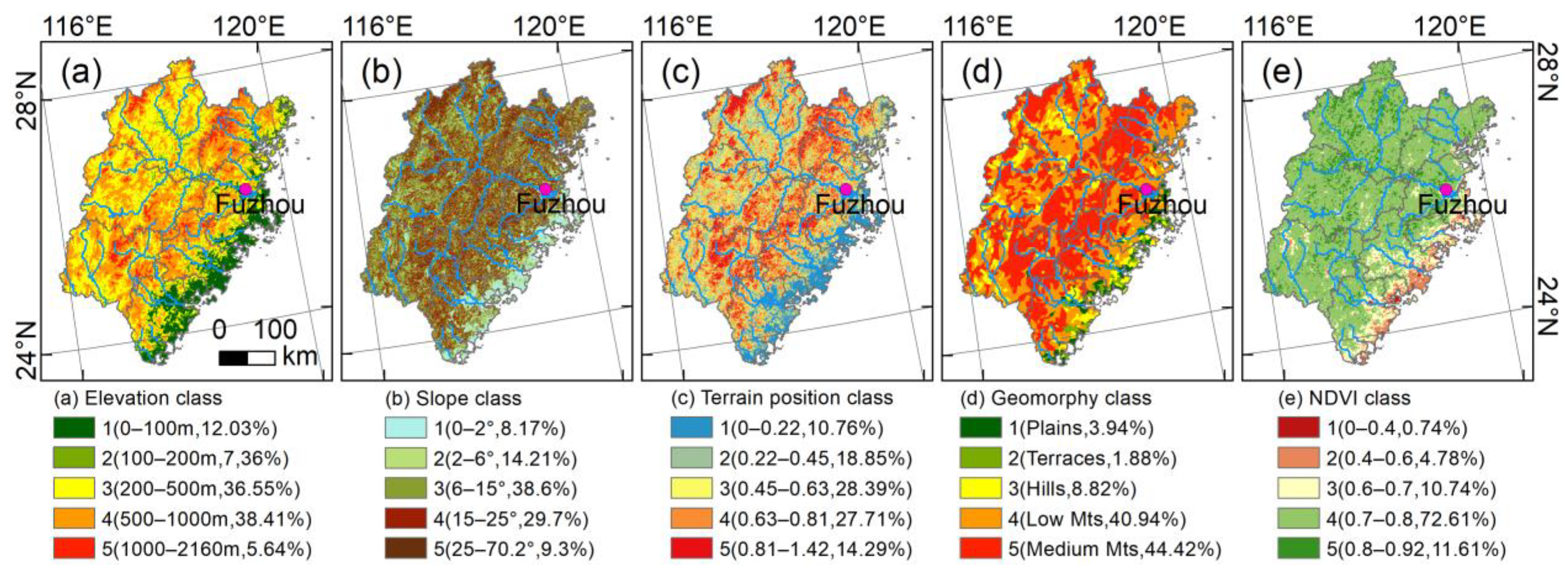
2.5.3. Environmental Factor Classification

The elevation, slope, terrain position index, and NDVI of the study area vary in the range of 0 to 2160 m, 0 to 70.2°, 0 to 1.42, and 0 to 0.92, respectively (Figure 4). Based on the commonly used grading standards of topographic and geomorphic features, the elevation is divided into five grades: 0 m to 100 m, 100 m to 200 m, 200 m to 500 m, 500 m to 1000 m, and 1000 m to 2160 m, respectively (Figure 4a). The slope is divided into five grades: 0° to 2°, 2° to 6°, 6° to 15°, 15° to 25°, and 25° to 70.2°, respectively (Figure 4b). Terrain position index is divided into 5 grades by the natural breaks (Jenks) method, which are 0 to 0.22, 0.22 to 0.45, 0.45 to 0.63, 0.63 to 0.81, and 0.81 to 1.42, respectively (Figure 4c). Geomorphy is divided into five types: plains, terraces, hills, low mountains, and medium mountains, respectively (Figure 4d). LULC is divided into six types: cultivated land, forest land, grassland, water body, built-up land, and unused land, respectively (Figure 3g–i). NDVI is divided into five grades: 0 to 0.4, 0.4 to 0.6, 0.6 to 0.7, 0.7 to 0.8, and 0.8 to 0.92, respectively (Figure 4e). This study analyzed the distribution characteristics of ecosystem services of water yield and soil conservation at different gradients levels of elevation, slope, terrain position index, geomorphy, LULC, and NDVI. Among them, LULC and NDVI gradients used corresponding annual data.

2.6. Geographical Detector

The geographical detector (Geodetector, http://geodetector.cn/) is used to explore the spatial differentiation characteristics of ecosystem services and reveal their driving factors, which is achieved through four detector modules [68,69,70,71].

(1) Factor detection is used to evaluate the spatial heterogeneity of the dependent variable Y (ecosystem services), as well as to determine to what extent the driving factor X explains the spatial heterogeneity of the dependent variable Y. (2) Interaction detection is used to identify the interaction between different driving factors Xs, that is, to evaluate whether the combined effect of driving factors X1 and X2 will increase or decrease the explanatory power of the dependent variable ecosystem services Y or whether the impact of these driving factors on ecosystem services Y is independent of each other. The relationship between two factors can be divided into 5 categories: non-linear weakening, single factor non-linear weakening, double factor enhancement, and independent and non-linear enhancement, respectively. (3) Ecological detection is used to compare whether there is a significant difference in the impact of two driving factors X1 and X2 on the spatial distribution of ecosystem services Y. (4) Risk detection is used to determine whether there is a significant difference in the mean values of attributes between two sub regions within the layer of ecosystem service Y caused by environmental gradient factors.

In order to further explore the distribution characteristics of ecosystem services under different environmental gradients and their combined effects, this study is based on the Geodetector analysis of the distribution and changes degree of water yield and soil conservation in each environmental gradient (factor detection), the differences in combining environmental gradients (interaction detection), the comparison of whether there are differences between different environmental gradients (ecological detection), and using the larger value in different environmental gradients as important region (risk detection). After comparing different grid sizes, the study area was divided into a 10 km × 10 km grid (Figure 1c), and ecosystem services and changes, as well as environmental gradient levels, were extracted into the grid for calculation.

3. Results

3.1. Water Yield Service

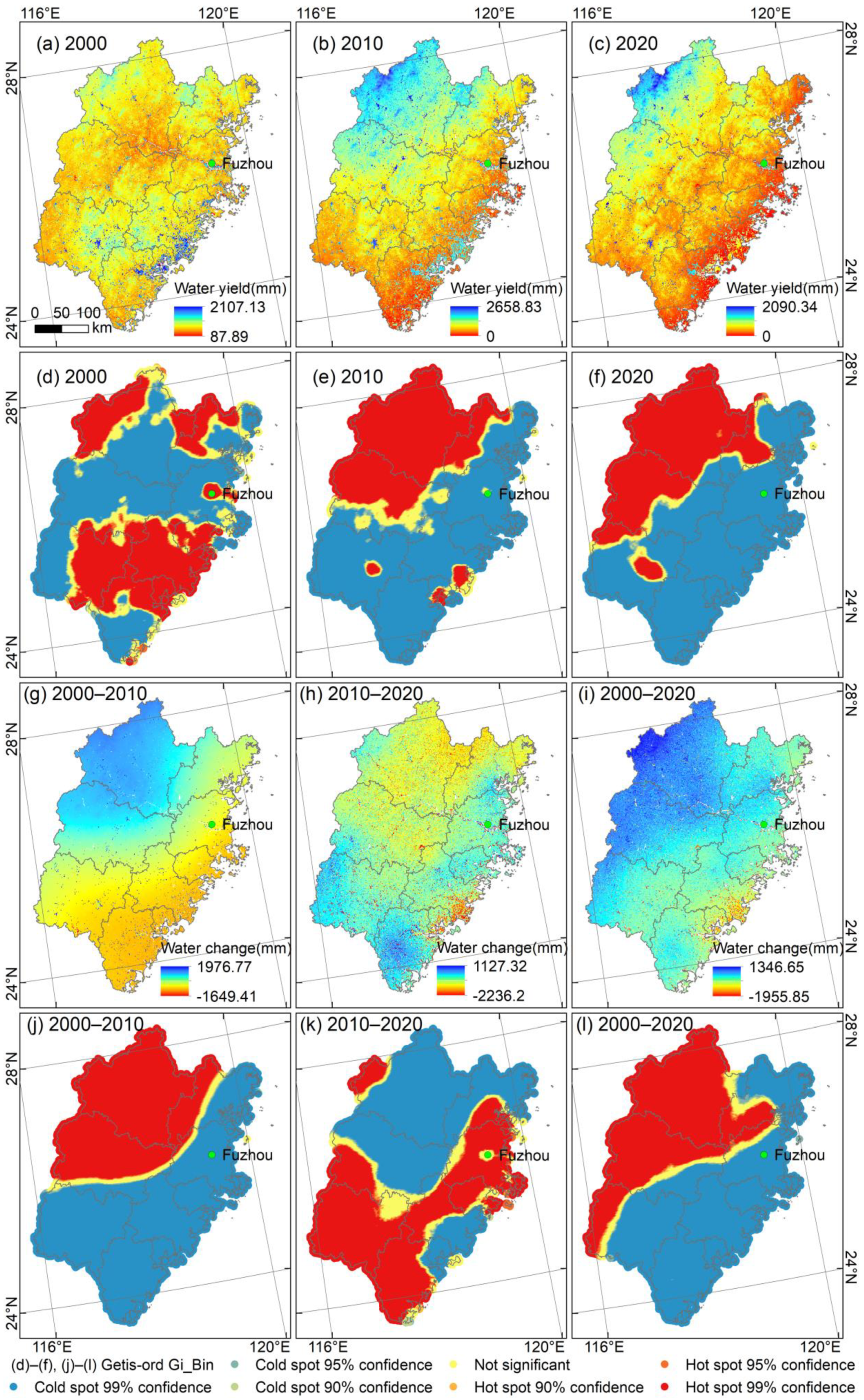
3.1.1. Spatial–Temporal Distribution of Water Yield

There were significant differences in water yield distribution of ecosystem in Fujian Province from 2000 to 2020 (Figure 5a–f), and the global Moran’s I and Z score also showed significant aggregation characteristics (

Table 3. Spatial correlation and clustering index of water yield in Fujian Province.

	2000	2010	2020	2000–2010	2010–2020	2000–2020
Global Moran’s I	0.239	0.557	0.498	0.857	0.277	0.558
Z score	1175.4	2737.6	3680.7	4210.2	1357.1	2727.9
p value	0.000	0.000	0.000	0.000	0.000	0.000

). In 2000, the water yield ranged from 87.89 mm to 2107 mm (mean 861.8 mm), with low values of water yield distributed in the southwest, extending towards the central and eastern parts, as well as the south, forming cold spot and clusters, while high values of water yield were distributed along the southeast coast, extending southwest, and locally in the north, forming hot spots and clusters (Figure 5a,d). In 2010 and 2020, the water yield ranged from 0 mm to 2658 mm (mean 994.6 mm) and 0 mm to 2090 mm (mean 460.7 mm), respectively. The low values of water yield were widely distributed in the southwest, south, and northeast, forming cold spots and clusters, while high value of water yield were distributed in the northwest, forming hot spots and clusters (Figure 5b,c,e,f).

3.1.2. Spatial–Temporal Changes in Water Yield

There were also significant differences in water yield changes in the ecosystem in Fujian Province from 2000 to 2020 (Figure 5g–l), and the Global Moran’s I and Z scores also showed significant aggregation characteristics (Table 3). The regions with decreased water yield from 2000 to 2010 were widely distributed in the southwest, south, and northeast, and formed cold spots and clusters, while the regions with increased yield were distributed in the northwest, and formed hot spots and clusters (Figure 5g,j). Unlike from 2000 to 2010, the regions with decreased water yield from 2010 to 2020 were mainly distributed in the central and northern regions, forming cold spots and clusters, while the regions with increased yields were distributed from southwest to northeast, forming hot spots and clusters (Figure 5h,k). The regions with decreased water yield over the entire study period from 2000 to 2020 were distributed in the northwest and slightly extended to the southwest, and formed cold spots and clusters, while the regions with increased yield were distributed in the east and south, forming hot spots and clusters (Figure 5i,l).

3.1.3. Water Yield Differences in Different Cities

There are significant differences in the water yield distribution and changes in the ecosystem in different cities in Fujian Province from 2000 to 2020 (Figure 6). The difference in water yield distribution range among different cities in 2000 was relatively small, and the average value showed that Xiamen and Quanzhou had relatively higher water production (Figure 6a). In 2010, there were significant differences in the water yield distribution range among different cities, and the average value showed that the water yield in the cities Nanping and Sanming were relatively high. The difference in water yield distribution range among different cities in 2020 was relatively small and low overall. The average value shows that the water production in Nanping and Sanming cities is relatively high, but lower than in 2000 and 2010.

The differences in water yield change between different cities from 2000 to 2010 are relatively small in range, and the average value shows increased water yields in Nanping and Sanming (Figure 6b). The differences in water yield change between different cities from 2010 to 2020 and from 2000 to 2020 were relatively large in range, with the average showing a decrease in water production in each city. The water yield fluctuations in Nanping and Sanming were more pronounced.

3.2. Soil Conservation Service

3.2.1. Spatial–Temporal Distribution of Soil Conservation

There were no significant differences in the soil conservation distribution of ecosystem in Fujian Province from 2000 to 2020 (Figure 7a–f), and the global Moran’s I and Z scores showed significant aggregation characteristics (

Table 4. Spatial correlation and clustering index of soil conservation in Fujian Province.

	2000	2010	2020	2000–2010	2010–2020	2000–2020
Global Moran’s I	0.218	0.258	0.197	0.574	0.119	0.2
Z score	683.6	810.1	1467.4	1803.2	588.2	989.7
p value	0.000	0.000	0.000	0.000	0.000	0.000

). The soil conservation amounts in 2000, 2010, and 2020 were 0 to 9432 t/km²·a (mean 1390.1 t/km²·a), 0 to 12,025 t/km²·a (mean 1491.8 t/km²·a), and 0 to 9992 t/km²·a (mean 1075.4 t/km²·a), respectively. The low values of soil conservation were distributed in the eastern coastal and southwestern regions and formed cold spots and clusters, while the high values were distributed in the northern and central regions, forming hot spots and clusters (Figure 7d–f). The hot spots and clusters were relatively fragmented in 2000 and 2010 (Figure 7d,e).

3.2.2. Spatial–Temporal Changes in Soil Conservation

There were significant differences in soil conservation changes in the ecosystem in Fujian Province from 2000 to 2020 (Figure 7g–l), and the global Moran’s I and Z scores also showed significant aggregation characteristics (Table 4). The regions with decreased soil conservation from 2000 to 2010 were widely distributed in the southwest, south, and northeast, forming cold spots and clusters, while the regions with increased conversation were distributed in the northwest, forming hot spots and clusters (Figure 7g,j). Unlike the period between the years 2000 and 2010, the regions with decreased soil conservation from 2010 to 2020 were distributed in the north and south, forming cold spots and clusters, while the regions with increased conservation were distributed in the southwest and southeast, forming hot spots and clusters (Figure 7h,k). The regions with decreased water yield over the entire study period, from 2000 to 2020, were distributed from the southwest to the northeast, forming cold spots and clusters, while the regions with increased water yield were distributed from the northwest to the southwest, as well as along the southeast coast, and formed hot spots and clusters (Figure 7i,l).

3.2.3. Soil Conservation Differences in Different Cities

There were significant differences in the soil conservation distribution and changes in ecosystem in different cities in Fujian Province from 2000 to 2020 (Figure 8). The average soil conservation values in different cities in 2000, 2010, and 2020 were similar, but the distribution range varied significantly, and the soil conservation distribution range was larger in Nanping and smaller in Xiamen (Figure 8a). The range of soil conservation changes was also relatively large in Nanping City but was small in Xiamen, and the average changes were relatively similar between 2000 and 2010, between 2010 and 2020, and between 2000 and 2020 (Figure 8b).

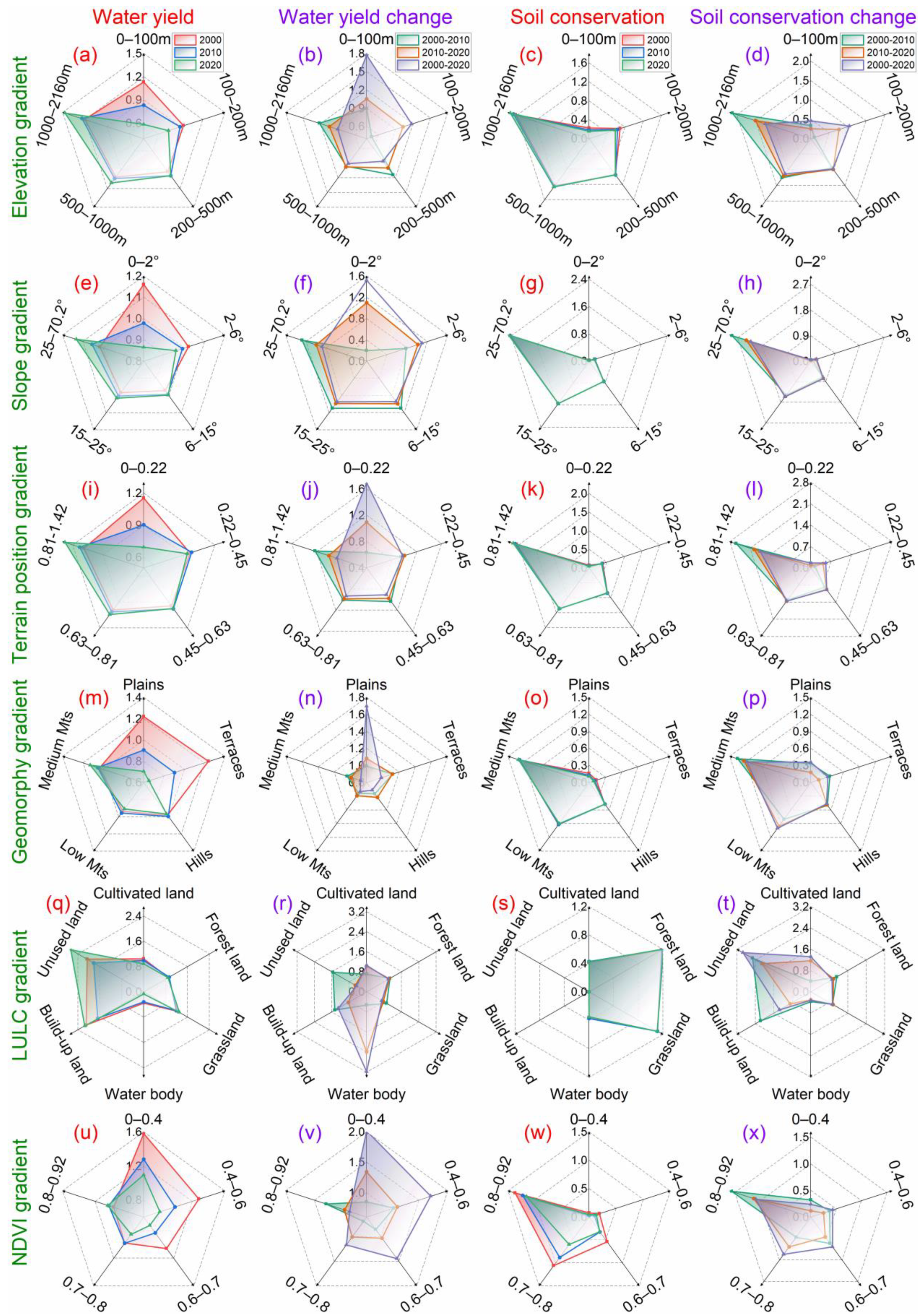
3.3. Gradient Distribution of Water Yield and Soil Conservation

3.3.1. Elevation Gradient Distribution

The elevation gradient distribution index of water yield distribution showed that the distribution indexes of water yield at low and high altitudes were relatively high, but there were interannual differences, and the differences in water yield distribution index at different elevations increased from 2000 to 2020 (Figure 9a). The decrease in the water yield distribution index was most significant at 0 m to 100 m, while the increase was most significant at 1000 m to 2160 m, and the water yield distribution index was basically stable at 200 m to 1000 m. The elevation gradient distribution index of water yield changes showed that the fluctuation of the distribution index of water yield changes at low altitudes was more significant, and while the difference in the distribution index of water yield changes at different elevations decreased, overall it was relatively large (Figure 9b). The distribution index of water yield change in 2000 to 2010 period was the lowest in a range of 100 to 200 m, with small differences in different elevation gradients from 2010 to 2020, and the differences across entire study period, from 2000 to 2020, were very high in a range 0 m to 100 m, but also reaching 100 m to 200 m.

The elevation gradient distribution index of soil conservation distribution showed that the higher the elevation, the higher the distribution index, and that the distribution indexes were very close across different years (Figure 9c). The distribution index of soil conservation at 1000 m to 2160 m was significantly higher than that of other ranges, followed by soil conservation at 500 m to 1000 m. The elevation gradient distribution index of soil conservation changes showed that the higher the elevation, the higher the distribution index, but the distribution index fluctuates significantly at different elevations (Figure 9d). The distribution index of soil conservation changes at 1000 m to 2160 m showed a significant decreasing trend, while at 100 m to 200 m showed an increasing trend.

3.3.2. Slope Gradient Distribution

The slope gradient distribution index of water yield distribution showed that the low slope and high slope had higher water yield distribution index, but there were interannual differences, and the differences in water yield distribution index among different slopes first decreased and then increased (Figure 9e). The decrease in water yield distribution index was most significant at 0° to 2°, while the increase was most significant at 25° to 70.2°, and the water yield distribution index was basically stable at 2° to 25°. The slope gradient of water yield changes showed that the fluctuation of the distribution index of water yield changes at low altitudes was more significant, and the distribution index of water yield changes at different slopes shows a decreasing trend, but overall, it was relatively large (Figure 9f). The distribution indexes of water production change from 2000 to 2010 were lowest at 0° to 2° and highest at 25° to 70.2°, there was little difference in different slope grades from 2010 to 2020, and the index for the entire research period from 2000 to 2020 was very high at 0° to 2°.

The slope gradient distribution index of soil conservation distribution and change showed that the higher the slope, the higher the distribution index, and the indexes were very similar in different years (Figure 9g,h). The distribution indexes of soil conservation and change at 25° to 70.2° were significantly higher than other ranges, followed by those at 15° to 25°. There was a slight decreasing trend in the distribution index of soil conservation changes at 25° to 70.2°.

3.3.3. Terrain Position Gradient Distribution

The terrain position gradient distribution index of water yield distribution showed that the water yield distribution indexes for low and high terrain positions were higher, but there were interannual differences, and the differences in water yield distribution indexes of different terrain positions first narrow and then increase (Figure 9i). The distribution index of water yield showed the highest and lowest values in 2000 and 2020 at 0 to 0.22 (level 1), respectively, with the most significant decrease. The distribution index of water yield showed the most significant increase at 0.81 to 1.42 (level 5), while the distribution index of water yield at 0.22 to 0.81 remained relatively stable. The terrain position gradient of water yield changes showed that the fluctuation of the distribution index of water yield changes in low terrain positions was more significant, followed by high terrain positions; the distribution index of water yield changes in different terrain positions shows a decreasing trend, but overall, it was relatively large (Figure 9j).

The terrain position gradient distribution index of soil conservation distribution and change showed that the higher the terrain position, the higher the distribution index, and the indexes were very similar across different years (Figure 9k,l). The distribution indexes of soil conservation and change at 0.81 to 1.42 (level 5) were significantly higher than other ranges, followed by that at 0.63 to 0.81. There was a slight decreasing trend in the distribution index of soil conservation changes at 0.81 to 1.42.

3.3.4. Geomorphic Gradient Distribution

The geomorphic gradient distribution index of water yield distribution showed that there was little difference in the distribution indexes of different geomorphic types, and the distribution index differences between terraces and plains showed a trend of first reducing and then increasing (Figure 9m). The water yield was highest in the terraces in 2000 and lowest in 2020, followed by the plains; the distribution index in hills, low mountains, and middle mountains were relatively similar. The geomorphic gradient of water yield changes shows that the distribution indexes of water yield at different stages (2000 to 2010 and 2010 to 2020) were relatively similar, while the differences across the entire research period from 2000 to 2020 were very obvious, and the distribution index of water yield changes on the plains was significantly higher than for other geomorphic types (Figure 9n).

The topographic gradient distribution index of soil conservation distribution and change showed that the distribution indexes for the plains and middle mountains were high, and the indexes were similar across different years (Figure 9o,p). The distribution index of soil conservation distribution and change was significantly higher for the middle mountains than for other topographic types, followed by the low mountains.

3.3.5. LULC Gradient Distribution

The LULC gradient distribution index of water yield distribution showed that the distribution indexes of different LULC types vary greatly (Figure 9q). The distribution index for built-up land and unused land were high, which indicates that the vast majority of precipitation is converted into runoff, while the distribution index for water bodies was low, and the distribution indexes for farmland, forest land, and grassland were similar. The LULC gradient distribution index of water yield changes showed that the fluctuations of the distribution index of water yield changes were more significant for different LULC types, especially for water bodies (Figure 9r). The distribution index difference was relatively small in the period from 2000 to 2010, while it was significantly larger from 2010 to 2020. The differences across the entire research period from 2000 to 2020 were more significant, with the largest difference observed for water bodies.

The LULC gradient distribution index of soil conservation distribution showed that the distribution indexes for different LULC types vary greatly (Figure 9s). The distribution indexes were significantly higher for forestland and grassland than for other LULC types, with a small level of distribution for cultivated land and water bodies, and almost none for built-up land and unused land. The LULC gradient distribution index of soil conservation changes also showed significant differences at different LULC types (Figure 9t). The distribution index showed little change at forestland, grassland, and water bodies, but were higher and fluctuates significantly at built-up land and unused land.

3.3.6. NDVI Gradient Distribution

The NDVI gradient distribution index of water yield distribution showed that as NDVI increased, the distribution index of water yield distribution decreased (Figure 9u). The distribution index was highest at 0 to 0.4 of NDVI, followed by 0.4 to 0.6, while the distribution index was lower but more stable and similar at 0.8 to 0.92. The NDVI gradient distribution index of water yield changes showed significant differences at the different stages and NDVI levels (Figure 9v). The distribution index of water yield changes was high at 0.8 and 0.92 from 2000 to 2010, relatively high at 0 to 0.4 from 2010 to 2020, and very high at 0 to 0.4 across the entire research period from 2000 to 2020, followed by 0.4 to 0.7.

The NDVI gradient distribution index of soil conservation distribution and change showed that as NDVI increased, the distribution index of soil conservation distribution was also increased, and there was a significant difference in the distribution index in different years (Figure 9w,x). The distribution index of soil conservation distribution and change was significantly higher at 0.8 to 0.92 than other NDVI levels, followed by 0.7 to 0.8. The distribution index of soil conservation slightly decreased at a level of 0.6 to 0.92, and the difference in distribution index of soil conservation changes showed a slight narrowing trend.

3.4. Spatial Differentiation of Distribution and Changes in Water Yield and Soil Conservation

3.4.1. Factor Detection

Factor detection q statistics showed that, in a single environmental gradient, the degree of water yield distribution and change (average 3.1% to 25.2%) was generally lower than that of soil conservation distribution and change (average 6.5% to 55.2%) (Figure 10, Table S1). The degree of distribution and change in water yield and soil conservation was generally more sensitive to terrain factors (slope, TPI, and DEM). The water yield distribution degree in 2000 was higher for the TPI (26.4%) and LULC gradients (21.8%); in 2010, it was relatively low overall, with relatively higher levels for the DEM (15%) and TPI gradients (14.8%); and in 2020, it was also higher for the DEM (24.5%) and TPI gradient (22.8%). There are differences in water yield change degree. From 2000 to 2010, there were higher levels in the DEM (21.6%), NDVI (21.6%), and TPI gradients (19.3%); from 2010 to 2020, the degree was relatively low overall, with slightly higher levels for the NDVI (6.9%) and LULC gradients (6.7%); and the entire research period from 2000 to 2020 showed high levels for the DEM (30.1%), NDVI (27.9%), and TPI (27.4%) gradients. The degree of water yield distribution and change were the lowest for the geomorphic gradient.

The highest degree of soil conservation distribution was observed in 2000, especially in terms of slope (73.4%), TPI (70.4%), and geomorphic gradient (57.6%); in 2010, the distribution was highest for slopes (68.3%) and the TPI gradient (65.9%); and in 2020, it was also relatively high for slope (65.3%) and the TPI gradient (64.8%). There were significant differences in the degree of soil conservation change. From 2000 to 2010, the soil conservation change was relatively low, with relatively higher levels for slopes (16.7%) and the NDVI gradient (16.5%); from 2010 to 2020, the change was relatively high in terms of slope (50.4%), TPI (44.6%), and geomorphic gradient (36.7%); and for the entire research period, from 2000 to 2020, the change degree was also relatively low, but was relatively higher in the slopes (12.8%) and the geomorphic gradient (9.3%). The degree of soil conservation distribution and change was the lowest for the LULC gradient.

3.4.2. Interaction Detection

The interaction detection of environmental gradients showed that there were two types of degree of water yield distribution and change: dual factor enhancement and non-linear enhancement (Figure 11, Table S2). In the interaction detection of different environmental gradients, the water yield distribution degree in 2000 was the highest, followed by the water yield change degree from 2000 to 2020, the water yield distribution degree in 2020, and the water yield change degree from 2000 to 2010. These are all dual factor enhancements, indicating that the degree of water yield distribution and change during these periods were higher than single factor detection results. The lowest was the water yield change degree from 2010 to 2020, but this factor exhibits significant non-linear enhancements, indicating that the water yield change degree during this period was more significant than the sum results of single factor detection.

The dominant effects of interaction detection vary in different periods of water yield. The water yield distribution degree in 2000 was higher for TPI∩LULC (38.3%), TPI∩NDVI (35.6%), DEM∩LULC (34.2%), geomorphy∩LULC (32.2%), and DEM∩NDVI (30.4%), while the interaction detection between slope and other environmental gradients was lower; in 2010 and 2020, the interaction detection between DEM and other environmental gradients was higher, while the interaction detection between slope and geomorphy with other environmental gradients was lower. The water yield change degree showed a higher interaction detection between NDVI and other environmental gradients from 2000 to 2010, while geomorphy had a lower interaction detection with other environmental gradients; from 2010 to 2020, the overall trend was relatively low, with a relatively high interaction detection between LULC and NDVI with other environmental gradients; and the interaction detection between DEM and other environmental gradients was relatively high throughout the entire research period from 2000 to 2020, while the interaction detection between slope and geomorphy with other environmental gradients was relatively low.

Environmental gradient interaction detection shows that the degree of soil conservation distribution and change was mainly achieved through dual factor enhancement, with only a small amount through non-linear enhancement (Figure 11, Table S2). In the interaction detection of different environmental gradients, the soil conservation distribution levels in 2000, 2010, and 2020 were all relatively high, significantly higher than the soil conservation change degree. The soil conservation distribution degree in 2000, 2010, and 2020, as well as the soil conservation change degree from 2000 to 2010 and from 2010 to 2020, all showed a dual factor enhancement, indicating that the degree of soil conservation distribution and change during these periods were higher than that of single factor detection results. The lowest was the soil conservation change degree across the entire research period from 2000 to 2020, but this exhibited non-linear enhancement, indicating that the degree of soil conservation change during this period was more significant than the sum results of single factor detection.

The dominant effects of interaction detection vary across different periods of soil conservation. The soil conservation distribution degree was found to be higher for the interaction detection between slope and other environmental gradients in 2000 and 2010, especially for slope∩TPI (82.3% in 2000), while the interaction detection between DEM and other environmental gradients was lower; in 2020, there were higher slope∩TPI (75.9%), DEM∩slope (74.5%), and slope∩geomorphy (70%) values, while the interaction detection between LULC and NDVI with other environmental gradients was lower. The soil conservation change degree was higher for NDVI interaction detection with other environmental gradients from 2000 to 2010 but was lower for the interaction detection of geomorphy and LULC with other environmental gradients; from 2010 to 2020 and throughout the entire research period from 2000 to 2020, the interaction detection between slope and other environmental gradients was high, while the interaction detection between LULC and NDVI with other environmental gradients was relatively low.

3.4.3. Ecological Detection

Ecological detection showed that there were significant differences in the degree of distribution and change in water yield and soil conservation for any two environmental gradients compared to each other; however, there were differences in results between different environmental gradients and between the same environmental gradients at different times (Figure 12, Table S3). The water yield distribution degree had greater differences in DEM, slope, geomorphy, LULC, and NDVI, when compared with other environmental gradients in sequence; the difference in TPI was greater compared to the DEM and slope. The water yield change degree was more significant for DEM, slope, TPI, geomorphy, LULC, and NDVI, when compared with other environmental gradients in sequence; the differences were inconsistent in comparison with geomorphy, LULC, and NDVI.

The soil conservation distribution degree showed greater differences in slope compared to DEM, in TPI compared to DEM, and in NDVI compared to LULC. The soil conservation change degree were greater differences in slope compared to DEM, and in geomorphy compared to DEM.

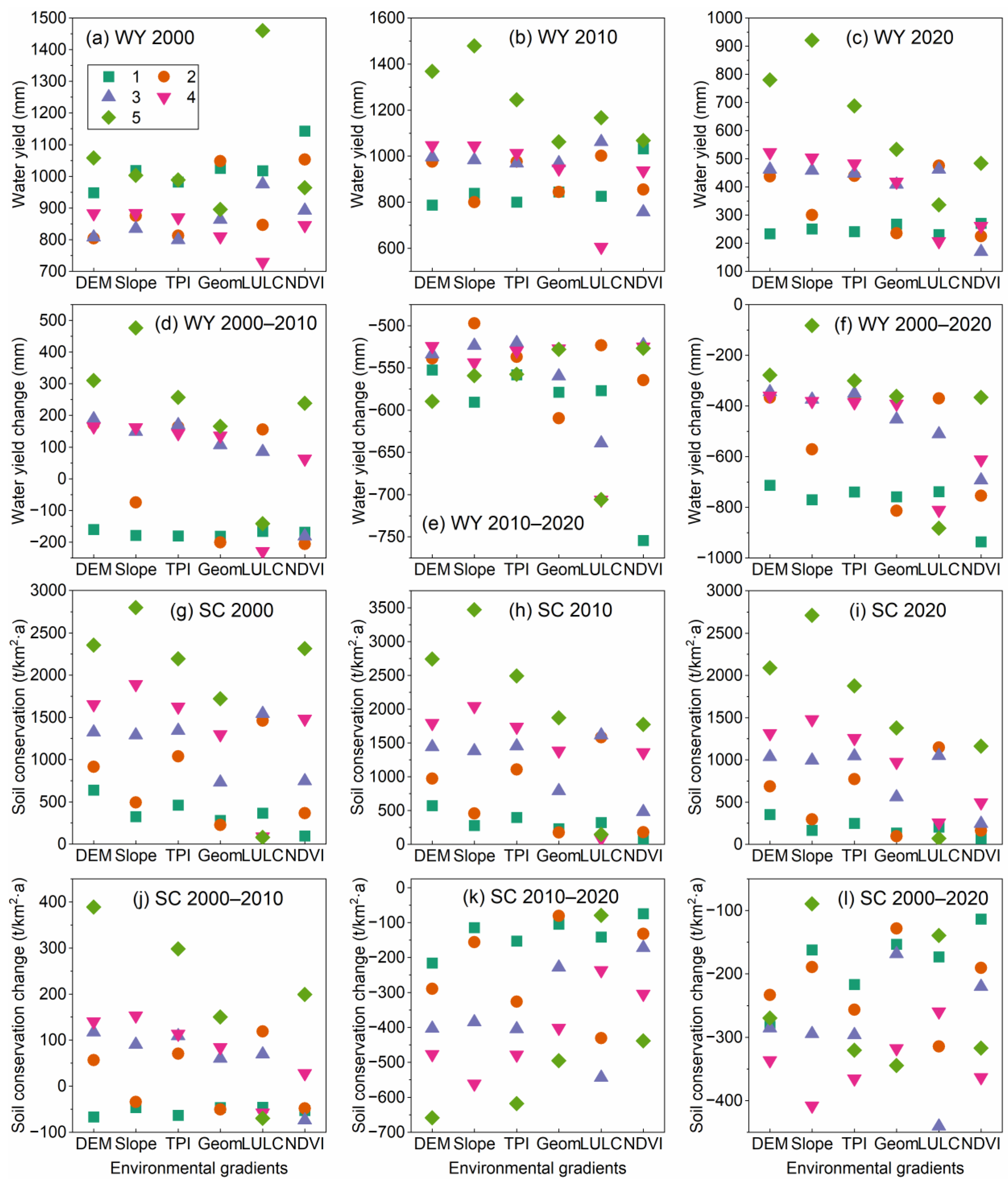
3.4.4. Risk Detection

The risk detection results showed that there were fluctuations in the high-value important regions of water yield and soil conservation in different environmental gradients (Figure 13, Table S4). The high-value important regions of water yield distribution were grade 5 in DEM, grades 1 and 5 in slope, grade 5 in TPI, categories 2 and 5 in geomorphy, categories 2 and 5 in LULC, and grades 1 and 5 in NDVI (

Table 5. High value important regions of distribution and change in water yield and soil conservation in Fujian Province based on risk detection.

	DEM	Slope	TPI	Geomorphy	LULC	NDVI
WY 2000	5	1	5	2	5	1
WY 2010	5	5	5	5	5	5
WY 2020	5	5	5	5	2	5
WY 2000–2010	5	5	5	5	2	5
WY 2010–2020	4	2	3	2	2	2
WY 2000–2020	5	5	5	5	2	5
WY overall	5 (1000–2160 m)	5 (25°–70.2°)	5 (0.81–1.42)	5 (medium mountain)	2 (forest land)	5 (0.9–0.92)
SC 2000	5	5	5	5	3	5
SC 2010	5	5	5	5	3	5
SC 2020	5	5	5	5	2	5
SC 2000–2010	5	4	5	5	2	5
SC 2010–2020	1	1	1	2	5	1
SC 2000–2020	2	5	1	2	5	1
SC overall	5 (1000–2160 m)	5 (25°–70.2°)	5 (0.81–1.42)	5 (medium mountain)	2 and 3 (forest land and grassland)	5 (0.9–0.92)

); the high-value important regions of water yield changes were grades 4 and 5 in DEM, grades 2 and 5 in slope, grades 3 and 5 in TPI, categories 2 and 5 in geomorphy, category 2 in LULC, and grades 2 and 5 in NDVI. Overall, the high-value important regions of water yield were 1000 to 2160 m (grade 5) in DEM, 25° to 70.2° (grade 5) in slope, 0.81 to 1.42 (grade 5) in TPI, medium mountain (category 5) in geomorphy, forest land (category 2) in LULC, and 0.9 to 0.92 (grade 5) in NDVI (Table 5, Figure 4).

The high-value important regions of soil conservation distribution were grade 5 in DEM, grade 5 in slope, grade 5 in TPI, category 5 in geomorphy, categories 2 and 3 in LULC, and grade 5 in NDVI (Table 5). The high-value important regions of soil conservation change were grades 1, 2, and 5 in DEM; grades 1, 4, and 5 in slope; grades 1 and 5 in TPI; categories 2 and 5 in geomorphy; categories 2 and 5 in LULC; and grades 1 and 5 in NDVI. Overall, the high-value important regions of soil conservation were 1000 to 2160 m (grade 5) in DEM, 25° to 70.2° (grade 5) in slope, 0.81 to 1.42 (grade 5) in TPI, medium mountain (category 5) in geomorphy, forest land and grassland (categories 2 and 3) in LULC, and 0.9 to 0.92 (grade 5) in NDVI (Table 5, Figure 4).

4. Discussion

4.1. Spatial–Temporal Characteristics of Water Yield and Soil Conservation

There was significant spatial heterogeneity in the water yield distribution in Fujian Province, and there were significant annual variations (Figure 5). Compared to the input materials of the InVEST model, there may be a relatively clear correlation with the high variability of precipitation data (Figure 3). In the Wuyi Mountain area in the west of Fujian Province, water yields also showed obvious spatial differences and temporal changes, and with the advancement of urbanization and economic development, water yield service capacity declined, and its flow to the human social system was weakened due to external interference [72]. Studies in Fujian and several neighboring provinces have shown significant differences in ecosystem services related to water yield in changes driven by precipitation factors [73]. In addition, soil conservation studies in other regions of South China have shown that climate change and LULC changes have a significant impact on water yield, especially with the most significant changes in precipitation [12,13,28,30,31].

There was also significant spatial heterogeneity in the soil conservation distribution in Fujian Province, but the annual variation was not significant (Figure 7). The spatial differences in soil erosion and soil conservation were also reflected in Guangdong and Jiangxi in South China [39,46]. Similarly, by comparing the input materials of the InVEST model, it can also be inferred that there was a connection to the precipitation erosivity changes caused by precipitation changes (Figure 3). Previous studies have shown that there are spatial differences in soil erosion vulnerability in Changting, Fujian [44]. The degree of soil erosion vulnerability gradually decreased from 1999 to 2015 [53], but it was still in a slightly fragile state and should tend to improve in the future [74]. Policy orientation affects the intensity of soil erosion, which in turn affects soil erosion [48]; in addition, terrain, meteorology, and economic and social variables are the main driving factors of ecological vulnerability [74]. Natural and human factors have a significant impact on the spatial variation in soil erosion, especially regarding land use and vegetation cover [75]. Research on soil conservation in other regions of South China has shown that natural environmental factors such as precipitation, slope, and terrain fluctuations [36,40,41], as well as economic development and agricultural yield, are important factors in soil erosion [9].

4.2. Gradient Effects of Water Yield and Soil Conservation

Previous studies have shown that altitude affects the supply and demand pattern of water yield, as well as the synergistic relationship with other ecosystem services [72,73]. The spatial differences in soil erosion and soil conservation displayed may be related to environmental backgrounds, such as vegetation cover, land use types, altitude, and slope [39,40,46]. Therefore, it is necessary to analyze the environmental gradient of ecosystem services.

The distribution index of environmental gradients showed that the distribution and change in water yield are very complex. The high values of water yield distribution were found mainly in higher levels (or categories) at elevation, slope, TPI, geomorphy, and LULC, except for the water production in 2010, which was at a low level for NDVI. The high values of water yield changes were distributed acro both low and high altitudes (Figure 9). The high values of soil conservation distribution and change were all at higher levels (or categories) for elevation, slope, TPI, geomorphy, and NDVI, while for LULC, soil conservation distribution was mainly high in forest and grassland, while soil conservation changes were higher in unused land (Figure 9). The distribution and changes in water yield and soil conservation were consistent with the risk detection results of Geodetector (Figure 13, Table 5). In addition, they all showed varying degrees of enhancement under the interaction of environmental gradients, and the distribution and changes in water yield and soil conservation were higher than those in a single environmental gradient (Figure 11). These results further indicate that ecosystem services exhibit spatiotemporal differences in distribution across different environmental gradients.

4.3. Research Inspiration and Prospects

This study explored the distribution and changes in water yield and soil conservation. Through comparison with other studies, it was found that natural environmental factors, such as precipitation, had a significant impact on water yield and soil conservation. Meanwhile, this study also analyzed the spatiotemporal patterns of distribution and changes for water yield and soil conservation in terms of six environmental gradients, which further supported the spatiotemporal differentiation of ecosystem services. Therefore, when conducting water yield and soil conservation assessments, simulations, and monitoring, control groups should be added for different environmental gradients to obtain more accurate research results. In addition, this study also suggests that when developing and utilizing the ecological environment, especially in mountainous and hilly areas where the ecological environment is fragile, humans should attempt to adapt to local conditions, carry out rational development, and have a long-term planning perspective.

However, this study focuses on water yield and soil conservation and fails to fully reflect the environmental gradient of ecosystem services. In addition, the complexity of ecosystem services and the diversity of driving factors pose significant challenges for the comprehensive assessment and understanding of ecosystem services. Therefore, in the future, it will be necessary to consider evaluating multiple ecosystem services, practicing in different research areas, conducting comparative studies using various methods, and analyzing driving forces to obtain a more complete and scientific understanding.

5. Conclusions

This study was based on the InVEST model to evaluate the water yield and soil conservation in Fujian Province in 2000, 2010, and 2020. The spatiotemporal distribution, changes, and urban differences in water yield and soil conservation were analyzed, and their differences were analyzed in regard to six environmental gradients: elevation, slope, terrain, topography, land use and land cover change, and normalized vegetation index.

(1)

There was a significant spatiotemporal distribution and variation difference in water yield from 2000 to 2010, and it revealed obvious clustering characteristics of cold and hot spots (low and high values). In 2010 and 2020, the water yield was higher in the north and lower in the south. From 2000 to 2020, the water yield increased in the north and decreased in the southeast. There were significant differences in the distribution and changes in water yield among different cities, with higher water yields and more significant changes in water yield in northern mountainous cities.

(2)

From 2000 to 2010, the soil conservation was high in the north and low in the south, without significant spatiotemporal changes, and also exhibited distinct clustering characteristics of cold and hot spots (low and high values). From 2000 to 2020, soil conservation changes slightly decreased in the north and slightly increased in the south. The distribution and change in soil conservation vary slightly among different cities, while soil conservation and change were relatively high in northern mountainous cities.

(3)

The distribution index of environmental gradients showed that the distribution and change in water yield were very complex. The high values of water yield distribution were mainly observed at higher levels (or categories) for elevation, slope, TPI, geomorphy, and LULC, except for the 2010 water geomorphy, which was at a low level at NDVI; the high values of water yield changes were distributed at both low and high altitudes. The high values of soil conservation distribution and change were all found at higher levels (or categories) for elevation, slope, TPI, topography, and NDVI. In LULC, soil conservation distribution was mainly higher in forest and grassland, while soil conservation changes were higher in unused land.

(4)

The factor detection of geographic detectors shows that at a single environmental gradient, the degrees of water yield distribution and change were generally lower than that of soil conservation, and the degrees of distribution and change in water yield and soil conservation were usually more sensitive to terrain factors (slope, TPI, and DEM). The interactive detection of environmental gradients indicates that there were two types of distribution and changes in water and soil conservation in different environments: dual factor enhancement and non-linear enhancement. Ecological detection showed that there were significant differences in the degrees of distribution and change in water yield and soil conservation in any two environmental gradients compared to each other; however, there were differences in results between different environmental gradients and between the same environmental gradients at different times. The risk detection results showed that there were fluctuations in the high-value important regions of water yield and soil conservation for different environmental gradients; the high-value important regions of water yield and soil conservation were 1000 to 2160 m (grade 5) for DEM, 25° to 70.2° (grade 5) for slope, 0.81 to 1.42 (grade 5) for TPI, medium mountain (category 5) for geomorphy, forest land (category 2) for LULC, and 0.9 to 0.92 (grade 5) for NDVI.

References

1. Gómez-Baggethun, E.; Barton, D.N. Classifying and valuing ecosystem services for urban planning. Ecol. Econ. 2013, 86, 235–245. [Google Scholar] [CrossRef]
2. Lee, H.; Lautenbach, S. A quantitative review of relationships between ecosystem services. Ecol. Indic. 2016, 66, 340–351. [Google Scholar] [CrossRef]
3. Tan, P.Y.; Zhang, J.; Masoudi, M.; Alemu, J.B.; Edwards, P.J.; Grêt-Regamey, A.; Richards, D.R.; Saunders, J.; Song, X.; Wong, L.W. A conceptual framework to untangle the concept of urban ecosystem services. Landsc. Urban Plan. 2020, 200, 103837. [Google Scholar] [CrossRef] [PubMed]
4. Liu, C.; Li, W.; Zhu, G.; Zhou, H.; Yan, H.; Xue, P. Land use/land cover changes and their driving factors in the Northeastern Tibetan Plateau based on Geographical Detectors and Google Earth Engine: A case study in Gannan Prefecture. Remote Sens. 2020, 12, 3139. [Google Scholar] [CrossRef]
5. Hasan, S.S.; Zhen, L.; Miah, M.G.; Ahamed, T.; Samie, A. Impact of land use change on ecosystem services: A review. Environ. Dev. 2020, 34, 100527. [Google Scholar] [CrossRef]
6. Wang, X.; Liu, G.; Xiang, A.; Qureshi, S.; Li, T.; Song, D.; Zhang, C. Quantifying the human disturbance intensity of ecosystems and its natural and socioeconomic driving factors in urban agglomeration in South China. Environ. Sci. Pollut. Res. 2022, 29, 11493–11509. [Google Scholar] [CrossRef]
7. Wang, X.; Liu, G.; Zhang, C.; Liao, Y. Spatial-temporal pattern and urban-rural gradient of comprehensive ecological security in urban agglomeration in South China from 2000 to 2020. Environ. Sci. Pollut. Res. 2023, 30, 102474–102489. [Google Scholar] [CrossRef]
8. Wang, X.; Zhong, W.; Wang, B.; Quan, M.; Li, T.; Lin, D.; Shang, S.; Zhu, C.; Zhang, C.; Liao, Y. Spatial–temporal variations and pollution risks of mercury in water and sediments of urban lakes in Guangzhou City, South China. Environ. Sci. Pollut. Res. 2022, 29, 80817–80830. [Google Scholar] [CrossRef]
9. Yu, Y.; Chen, X.; Malik, I.; Wistuba, M.; Cao, Y.; Hou, D.; Ta, Z.; He, J.; Zhang, L.; Yu, R.; et al. Spatiotemporal changes in water, land use, and ecosystem services in Central Asia considering climate changes and human activities. J. Arid Land 2021, 13, 881–890. [Google Scholar] [CrossRef]
10. Millennium Ecosystem Assessment (MEA). Ecosystems and Human Well-Being: Synthesis; Island Press: Washington, DC, USA, 2005. [Google Scholar]
11. Hu, Y.; Gao, M. Evaluations of water yield and soil erosion in the Shaanxi-Gansu Loess Plateau under different land use and climate change scenarios. Environ. Dev. 2020, 34, 100488. [Google Scholar] [CrossRef]
12. Wang, X.; Liu, G.; Lin, D.; Lin, Y.; Lu, Y.; Xiang, A.; Xiao, S. Water yield service influence by climate and land use change based on InVEST model in the monsoon hilly watershed in South China. Geomat. Nat. Hazards Risk 2022, 13, 2024–2048. [Google Scholar] [CrossRef]
13. Wang, Z.; Li, Q.; Liu, L.; Zhao, H.; Ru, H.; Wu, J.; Deng, Y. Spatiotemporal evolution and attribution analysis of water yield in the Xiangjiang River Basin (XRB) based on the InVEST model. Water 2023, 15, 514. [Google Scholar] [CrossRef]
14. Fang, Z.; Ding, T.; Chen, J.; Xue, S.; Zhou, Q.; Wang, Y.; Wang, Y.; Huang, Z.; Yang, S. Impacts of land use/land cover changes on eco-system services in ecologically fragile regions. Sci. Total Environ. 2022, 831, 154967. [Google Scholar] [CrossRef] [PubMed]
15. Ren, Q.; Liu, D.; Liu, Y. Spatio-temporal variation of ecosystem services and the response to urbanization: Evidence based on Shandong province of China. Ecol. Indic. 2023, 151, 110333. [Google Scholar] [CrossRef]
16. Sherrouse, B.C.; Semmens, D.J.; Clement, J.M. An application of Social Values for Ecosystem Services (SolVES) to three national forests in Colorado and Wyoming. Ecol. Indic. 2014, 36, 68–79. [Google Scholar] [CrossRef]
17. Sherrouse, B.C.; Semmens, D.J.; Ancona, Z.H. Social Values for Ecosystem Services (SolVES): Open-source spatial modeling of cultural services. Environ. Model. Softw. 2022, 148, 105259. [Google Scholar] [CrossRef]
18. Bagstad, K.J.; Villa, F.; Batker, D.; Harrison-Cox, J.; Voigt, B.; Johnson, G.W. From theoretical to actual ecosystem services: Mapping beneficiaries and spatial flows in ecosystem service assessments. Ecol. Soc. 2014, 19, 64. [Google Scholar] [CrossRef]
19. Capriolo, A.; Boschetto, R.G.; Mascolo, R.A.; Balbi, S.; Villa, F.J.E.S. Biophysical and economic assessment of four ecosystem services for natural capital accounting in Italy. Ecosyst. Serv. 2020, 46, 101207. [Google Scholar] [CrossRef]
20. Hu, Y.; Gong, J.; Li, X.; Song, L.; Zhang, Z.; Zhang, S.; Zhang, W.; Dong, J.; Dong, X. Ecological security assessment and ecological management zoning based on ecosystem services in the West Liao River Basin. Ecol. Eng. 2023, 192, 106973. [Google Scholar] [CrossRef]
21. He, Y.; Ma, J.; Zhang, C.; Yang, H. Spatio-temporal evolution and prediction of carbon storage in Guilin based on FLUS and InVEST models. Remote Sens. 2023, 15, 1445. [Google Scholar] [CrossRef]
22. Anley, M.A.; Minale, A.S. Modeling the impact of land use land cover change on the estimation of soil loss and sediment export using InVEST model at the Rib watershed of Upper Blue Nile Basin, Ethiopia. Remote Sens. Appl. Soc. Environ. 2024, 34, 101177. [Google Scholar] [CrossRef]
23. Jia, H.; Yang, S.; Liu, L.; Wang, R.; Li, Z.; Li, H.; Liu, J. Distinguishing the Multifactorial Impacts on Ecosystem Services under the Long-Term Ecological Restoration in the Gonghe Basin of China. Remote Sens. 2024, 16, 2460. [Google Scholar] [CrossRef]
24. Jia, H.; Yang, S.; Liu, L.; Li, H.; Li, Z.; Chen, Y.; Liu, J. Assessment and Prediction of Carbon Storage Based on Land Use/Land Cover Dynamics in the Gonghe Basin. Land 2024, 13, 2180. [Google Scholar] [CrossRef]
25. Li, T.; Zhong, W.; Quan, M.; Wang, X.; Yu, J. A 47.0-kyr record of mercury deposition in lake sediments from Dahu swamp in the East Nanling Mountains, southern China: Implications for paleoclimatic and environmental changes. J. Quat. Sci. 2025, 40, 9–21. [Google Scholar] [CrossRef]
26. Lin, D.; Zhong, W.; Wang, X.; Quan, M.; Li, T.; Zhang, E. Spatiotemporal characteristics and forcing mechanism of precipitation changes in the Nanling Mountains and surrounding regions in South China over the past 60 years. Theor. Appl. Climatol. 2025, 156, 57. [Google Scholar] [CrossRef]
27. Liu, G.; Xiang, A.; Wan, Z.; Zhang, L.; Wu, J.; Xie, Z. Quantitative characterization, spatiotemporal evolution, and analysis of driving factors of daily dry-wet abrupt alternation: A case study of the Ganjiang River Basin. J. Hydrol. Reg. Stud. 2024, 56, 102030. [Google Scholar] [CrossRef]
28. Lang, Y.; Song, W.; Zhang, Y. Responses of the water-yield ecosystem service to climate and land use change in Sancha River Basin, China. Phys. Chem. Earth 2017, 101, 102–111. [Google Scholar] [CrossRef]
29. Lang, Y.; Song, W.; Deng, X. Projected land use changes impacts on water yields in the karst mountain areas of China. Phys. Chem. Earth 2018, 104, 66–75. [Google Scholar] [CrossRef]
30. Yang, D.; Liu, W.; Tang, L.; Chen, L.; Li, X.; Xu, X. Estimation of water provision service for monsoon catchments of South China: Applicability of the InVEST model. Landsc. Urban Plan. 2019, 182, 133–143. [Google Scholar] [CrossRef]
31. Mo, W.; Zhao, Y.; Yang, N.; Xu, Z.; Zhao, W.; Li, F. Effects of climate and land use/land cover changes on water yield services in the Dongjiang Lake Basin. ISPRS Int. J. Geo-Inf. 2021, 10, 466. [Google Scholar] [CrossRef]
32. Yang, D.; Liu, W.; Xu, C.; Tao, L.; Xu, X. Integrating the InVEST and SDSM model for estimating water provision services in response to future climate change in monsoon basins of South China. Water 2020, 12, 3199. [Google Scholar] [CrossRef]
33. Wang, J.F.; Zhang, T.L.; Fu, B.J. A measure of spatial stratified heterogeneity. Ecol. Indic. 2016, 67, 250–256. [Google Scholar] [CrossRef]
34. Hu, W.; Li, G.; Gao, Z.; Jia, G.; Wang, Z.; Li, Y. Assessment of the impact of the Poplar Ecological Retreat Project on water conservation in the Dongting Lake wetland region using the InVEST model. Sci. Total Environ. 2020, 733, 139423. [Google Scholar] [CrossRef] [PubMed]
35. Gu, K.; Ma, L.; Xu, J.; Yu, H.; Zhang, X. Spatiotemporal Evolution Characteristics and Driving Factors of Water Conservation Service in Jiangxi Province from 2001 to 2020. Sustainability 2023, 15, 11941. [Google Scholar] [CrossRef]
36. He, X.; Miao, Z.; Wang, Y.; Yang, L.; Zhang, Z. Response of soil erosion to climate change and vegetation restoration in the Ganjiang River Basin, China. Ecol. Indic. 2024, 158, 111429. [Google Scholar] [CrossRef]
37. Li, H.; Chen, X.; Lim, K.J.; Cai, X.; Sagong, M. Assessment of soil erosion and sediment yield in Liao watershed, Jiangxi Province, China, Using USLE, GIS, and RS. J. Earth Sci. 2010, 21, 941–953. [Google Scholar] [CrossRef]
38. Yu, S.; Wang, L.; Zhao, J.; Shi, Z. Using structural equation modelling to identify regional socio-economic driving forces of soil erosion: A case study of Jiangxi Province, southern China. J. Environ. Manag. 2021, 279, 111616. [Google Scholar] [CrossRef]
39. Wang, X.; Liu, X.; Long, Y.; Liang, W.; Zhou, J.; Zhang, Y. Analysis of Soil retention service function in the North Area of Guangdong based on the InVEST model. IOP Conf. Ser. Earth Environ. Sci. 2020, 510, 032011. [Google Scholar] [CrossRef]
40. Li, H.; Shi, D. Spatio-temporal variation in soil erosion on sloping farmland based on the integrated valuation of ecosystem services and trade-offs model: A case study of Chongqing, southwest China. Catena 2024, 236, 107693. [Google Scholar] [CrossRef]
41. Guo, Z.; Yan, Z.; PaErHaTi, M.; He, R.; Yang, H.; Wang, R.; Ci, H. Assessment of soil erosion and its driving factors in the Huaihe region using the InVEST-SDR model. Geocarto Int. 2023, 38, 2213208. [Google Scholar] [CrossRef]
42. Dang, X.; Sui, B.; Gao, S.; Liu, G.; Wang, T.; Wang, B.; Ning, D.; Bi, W. Regions and their typical paradigms for soil and water conservation in China. Chin. Geogr. Sci. 2020, 30, 643–664. [Google Scholar] [CrossRef]
43. Hu, X.; Li, Z.; Nie, X.; Wang, D.; Huang, J.; Deng, C.; Shi, L.; Wang, L.; Ning, K. Regionalization of soil and water conservation aimed at ecosystem services improvement. Sci. Rep. 2020, 10, 3469. [Google Scholar] [CrossRef]
44. Chen, S.; Zha, X. Evaluation of soil erosion vulnerability in the Zhuxi watershed, Fujian Province, China. Nat. Hazards 2016, 82, 1589–1607. [Google Scholar] [CrossRef]
45. Wang, G.; Innes, J.; Yang, Y.; Chen, S.; Krzyzanowski, J.; Xie, J.; Lin, W. Extent of soil erosion and surface runoff associated with large-scale infrastructure development in Fujian Province, China. Catena 2012, 89, 22–30. [Google Scholar] [CrossRef]
46. Li, Z.; Ning, K.; Chen, J.; Liu, C.; Wang, D.; Nie, X.; Hu, X.; Wang, L.; Wang, T. Soil and water conservation effects driven by the implementation of ecological restoration projects: Evidence from the red soil hilly region of China in the last three decades. J. Clean. Prod. 2020, 260, 121109. [Google Scholar] [CrossRef]
47. Wang, H.; Chen, W.; Zhou, M.; Zhuo, Z.; Zhang, Y.; Jiang, F.; Huang, Y.; Lin, J. Runoff and sediment characteristics of a typical watershed after continuous soil erosion control in the red soil region of Southern China. Catena 2023, 233, 107484. [Google Scholar] [CrossRef]
48. Lin, C.; Zhou, S.L.; Wu, S.H.; Liao, F.Q. Relationships between intensity grada-tion and evolution of soil erosion: A case study of Changting in Fujian Province, China. Pedosphere 2012, 22, 243–253. [Google Scholar] [CrossRef]
49. Zhong, L.; Wang, J.; Zhang, X.; Ying, L.; Zhu, C. Effects of agricultural land consolidation on soil conservation service in the Hilly Region of Southeast China–Implications for land management. Land Use Policy 2020, 95, 104637. [Google Scholar] [CrossRef]
50. Chen, S.; Bai, Y.; Li, H.; Liu, W. Impact of farmers’ livelihood behavior on soil erosion in hilly areas—A comparison between erosion controlled and uncontrolled areas of southern China. Arab. J. Geosci. 2021, 14, 674. [Google Scholar] [CrossRef]
51. Wang, X.; Zhong, W.; Li, T.; Quan, M.; Wang, B.; Wei, Z. A 16.2-kyr lacustrine sediment record of mercury deposition in Dahu Swamp, eastern Nanling Mountains, southern China: Analysis of implications for climatic changes. Quat. Int. 2021, 592, 12–21. [Google Scholar] [CrossRef]
52. Wang, X.; Zhong, W.; Quan, M.; Li, T.; Lin, D.; Zhang, C. Asynchronous variations of mercury accumulation since the last deglaciation in the eastern and western Nanling mountains in South China. Quat. Sci. Rev. 2024, 325, 108490. [Google Scholar] [CrossRef]
53. Chen, S.; Zha, X.; Bai, Y.; Wang, L. Evaluation of soil erosion vulnerability on the basis of exposure, sensitivity, and adaptive capacity: A case study in the Zhuxi watershed, Changting, Fujian Province, Southern China. Catena 2019, 177, 57–69. [Google Scholar] [CrossRef]
54. Xu, X.; Liu, J.; Zhang, S.; Li, R.; Yan, C.; Wu, S. China Multi Period Land Use/Land Cover Remote Sensing Monitoring Dataset (CNLUCC); Data Registration and Publishing System of the Resource and Environmental Science Data Center of the Chinese Academy of Sciences: Beijing, China, 2018; (In Chinese). [Google Scholar] [CrossRef]
55. Li, S.; Su, S.; Liu, Y.; Zhou, X.; Luo, Q.; Paudel, B. Effectiveness of the Qilian Mountain nature reserve of China in reducing human impacts. Land 2022, 11, 1071. [Google Scholar] [CrossRef]
56. Trabucco, A.; Zomer, R. Global Aridity Index and Potential Evapotranspiration (ET0) Climate Database v3. Figshare. Dataset 2022. [Google Scholar] [CrossRef]
57. Hengl, T.; Mendes de Jesus, J.; Heuvelink, G.B.; Ruiperez Gonzalez, M.; Kilibarda, M.; Blagotić, A.; Shangguan, W.; Wright, M.N.; Geng, X.; Bauer-Marschallinger, B.; et al. SoilGrids250m: Global gridded soil information based on machine learning. PLoS ONE 2017, 12, e0169748. [Google Scholar] [CrossRef]
58. Xu, X. China Annual Normalized Difference Vegetation Index (NDVI) Spatial Distribution Dataset; Data Registration and Publishing System of the Resource and Environmental Science Data Center of the Chinese Academy of Sciences: Beijing, China, 2018; Available online: https://www.resdc.cn/DOI/doi.aspx?DOIid=49 (accessed on 20 March 2024). (In Chinese)
59. Sharp, R.; Douglass, J.; Wolny, S.; Arkema, K.; Bernhardt, J.; Bierbower, W.; InVEST 3.10.2 User’s Guide. The Natural Capital Project, Stanford University, University of Minnesota, The Nature Conservancy, and World Wildlife Fund. 2020. Available online: https://naturalcapitalproject.stanford.edu/software/invest (accessed on 10 January 2022).
60. Liu, M.; Dong, X.; Zhang, Y.; Wang, X.C.; Wei, H.; Zhang, P.; Zhang, Y. Spatiotemporal changes in future water yield and the driving factors under the carbon neutrality target in Qinghai. Ecol. Indic. 2024, 158, 111310. [Google Scholar] [CrossRef]
61. Zhang, L.; Hickel, K.; Dawes, W.R.; Chiew, F.H.; Western, A.W.; Briggs, P.R. A rational function approach for estimating mean annual evapotranspiration. Water Resour. Res. 2004, 40, W02502. [Google Scholar] [CrossRef]
62. Donohue, R.J.; Roderick, M.L.; McVicar, T.R. Roots, storms and soil pores: Incorporating key ecohydrological processes into Budyko’s hydrological model. J. Hydrol. 2012, 436, 35–50. [Google Scholar] [CrossRef]
63. Allen, R.G.; Pereira, L.S.; Raes, D.; Smith, M. Crop evapotranspiration-Guidelines for computing crop water requirements-FAO Irrigation and drainage paper 56. Fao Rome 1998, 300, D05109. [Google Scholar]
64. Qiao, X.; Li, Z.; Lin, J.; Wang, H.; Zheng, S.; Yang, S. Assessing current and future soil erosion under changing land use based on InVEST and FLUS models in the Yihe River Basin, North China. Int. Soil Water Conserv. Res. 2024, 12, 298–312. [Google Scholar] [CrossRef]
65. Chen, J.; Chen, Y.; Wang, K.; Zhang, H.; Tian, H.; Cao, J. Impacts of land use, rainfall, and temperature on soil con-servation in the Loess Plateau of China. Catena 2024, 239, 107883. [Google Scholar] [CrossRef]
66. Zhou, F.; Huang, Y. The R value of rainfall erosivity index in Fujian Province in China. J. Soil Water Conserv. 1995, 9, 13–18. Available online: http://stbcxb.alljournal.com.cn/stbcxb/article/abstract/19950103 (accessed on 20 March 2024). (In Chinese).
67. Wang, X.; Liu, G.; Xiang, A.; Xiao, S.; Lin, D.; Lin, Y.; Lu, Y. Terrain gradient response of landscape ecological envi-ronment to land use and land cover change in the hilly watershed in South China. Ecol. Indic. 2023, 146, 109797. [Google Scholar] [CrossRef]
68. Wang, J.F.; Li, X.H.; Christakos, G.; Liao, Y.L.; Zhang, T.; Gu, X.; Zheng, X.Y. Geographical detectors-based health risk assessment and its application in the neural tube defects study of the Heshun Region, China. Int. J. Geogr. Inf. Sci. 2010, 24, 107–127. [Google Scholar] [CrossRef]
69. Wang, X.; Dai, E.; Zhu, J. Spatial patterns of forest ecosystem services and influencing factors in the Ganjiang River Basin. J. Resour. Ecol. 2016, 7, 439–452. [Google Scholar] [CrossRef]
70. Wang, J.; Haining, R.; Zhang, T.; Xu, C.; Hu, M.; Yin, Q.; Li, L.; Zhou, C.; Li, G.; Chen, H. Statistical modeling of spatially stratified heterogeneous data. Ann. Am. Assoc. Geogr. 2024, 114, 499–519. [Google Scholar] [CrossRef]
71. Wang, J.F.; Xu, C.D. Geodetector: Principle and prospective. Acta Geogr. Sin. 2017, 72, 116–134. (In Chinese) [Google Scholar] [CrossRef]
72. Chen, X.; Lin, S.; Tian, J.; Wang, Y.; Ye, Y.; Dong, S.; Gong, X.; Lin, Q.; Zhu, L. Simulation study on water yield service flow based on the InVEST-Geoda-Gephi network: A case study on Wuyi Mountains, China. Ecol. Indic. 2024, 159, 111694. [Google Scholar] [CrossRef]
73. Liao, Q.; Li, T.; Liu, D. Evolutionary patterns and influencing factors of relationships among ecosystem services in the hilly red soil region of Southern China. Environ. Monit. Assess. 2024, 196, 360. [Google Scholar] [CrossRef]
74. Wu, X.; Zhu, C.; Yu, J.; Zhai, L.; Zhang, H.; Yang, K.; Hou, X. Ecological vulnerability in the red soil erosion area of Changting under continuous ecological restoration: Spatiotemporal dynamic evolution and prediction. Forests 2022, 13, 2136. [Google Scholar] [CrossRef]
75. Gao, J.; Shi, C.; Yang, J.; Yue, H.; Liu, Y.; Chen, B. Analysis of spatiotemporal heterogeneity and influencing factors of soil erosion in a typical erosion zone of the southern red soil region, China. Ecol. Indic. 2023, 154, 110590. [Google Scholar] [CrossRef]
Figure 1. Study area. (a) Location of Fujian Province in China; SASM, EASM, and EAWM represent South Asian Summer Monsoon, East Asian Summer Monsoon, and East Asian Winter Monsoon, respectively [51,52]. (b) City distribution in Fujian Province. (c) A 10 km × 10 km grid of Fujian Province.
Water 17 00230 g001
Figure 2. Research framework.
Water 17 00230 g002
Figure 3. Input data for water yield and soil conservation evaluation in Fujian Province. (ac) Annual precipitation from 2000 to 2020; (d) average annual potential evapotranspiration from 1970 to 2000; (e) root restriction depth; (f) plant available water content (PAWC); (gi) LULC from 2000 to 2020. CL, FL, GL, WB, BL, and UL represent cultivated land, forest land, grassland, water body, built-up land, and unused land, respectively; (j) DEM; (km) rainfall erosivity; (n) soil erodibility.
Water 17 00230 g003
Figure 4. Classification of environmental gradient index in Fujian Province. (a) Elevation; (b) slope; (c) terrain position index; (d) geomorphy; (e) NDVI in 2000. LULC data are shown in Figure 3g–i.
Water 17 00230 g004
Figure 5. Spatial–temporal distribution of water yield in Fujian Province from 2000 to 2020. (ac) Water yield distribution. (df) Cold and hot spot clustering analysis of water yield distribution. (gi) Water yield change. (jl) Cold and hot spot clustering analysis of water yield change.
Water 17 00230 g005
Figure 6. Range and mean of water yield in different cities in Fujian Province. (a) Water yield from 2000 to 2020 in different cities. (b) Water yield change from 2000 to 2020 in different cities.
Water 17 00230 g006
Figure 7. Spatial–temporal distribution of soil conservation in Fujian Province from 2000 to 2020. (ac) Soil conservation distribution. (df) Cold and hot spot clustering analysis of soil conservation distribution. (gi) Soil conservation change. (jl) Cold and hot spot clustering analysis of soil conservation change.
Water 17 00230 g007
Figure 8. Range and mean of soil conservation in different cities in Fujian Province. (a) Soil conservation from 2000 to 2020 in different cities. (b) Soil conservation change from 2000 to 2020 in different cities.
Water 17 00230 g008
Figure 9. Gradient distribution index of ecosystem services in Fujian Province from 2000 to 2020. (ad) Elevation gradient of water yield, water yield change, soil conservation, and soil conservation change. (eh) Slope gradient of water yield, water yield change, soil conservation, and soil conservation change. (il) Terrain position gradient of water yield, water yield change, soil conservation, and soil conservation change. (mp) Geomorphic gradient of water yield, water yield change, soil conservation, and soil conservation change. (qt) LULC gradient of water yield, water yield change, soil conservation, and soil conservation change. (ux) NDVI gradient of water yield, water yield change, soil conservation, and soil conservation change.
Water 17 00230 g009
Figure 10. Factor detection of spatial differentiation of distribution and changes in water yield and soil conservation in Fujian Province (the data are shown in Table S1).
Water 17 00230 g010
Figure 11. Interaction detection of spatial differentiation of distribution and changes in water yield and soil conservation in Fujian Province (the data are given in Table S2).
Water 17 00230 g011
Figure 12. Ecological detection of spatial differentiation of distribution and changes in water yield and soil conservation in Fujian Province (the data are shown in Table S3). Y indicates that the degree of distribution and changes in water yield and soil conservation are greater on the left than on the right, while N demonstrates the opposite.
Water 17 00230 g012
Figure 13. Risk detection of spatial differentiation of distribution and changes in water yield and soil conservation in Fujian Province (the data are given in Table S4).
Water 17 00230 g013