Abstract
Winter precipitation (P) in East Asia (EA) is characterized by a wetter south and a drier north. Most of the existing research has concentrated on elucidating the mechanisms of winter P in southern EA, with relatively less attention given to northern East Asia (NEA). Our analysis showed that the correlation coefficient (c.c.) of average winter precipitation anomaly percentage (PAP) between southern EA and NEA is 0.24 for the period 1950–2023, indicating substantial regional difference. An empirical orthogonal function (EOF) analysis was conducted on the winter PAP in NEA. The first and second mode (EOF1 and EOF2) account for 45.5% and 17.9% of the total variance, respectively. EOF1 is characterized by a region-wide uniform spatial pattern whereas EOF2 exhibits a north–south dipole pattern. Further analysis indicated that the two EOF modes are related to distinct atmospheric circulation and external forcings. Specifically, EOF1 is linked to a wave train from Central Siberia toward Japan, while EOF2 is connected with an anomaly similar to the Western Pacific pattern. Variations in mid–high latitude sea surface temperatures, sea ice, and snow are potential factors influencing EOF1. EOF2 exhibits a close relationship with tropical SST anomalies.
1. Introduction
In recent decades, East Asian winter precipitation (P) has been increasing, a trend that may be linked to global warming [1,2,3]. This winter P frequently causes severe freezing rain- and snow-related disasters [4,5,6]. For example, in November 2023, a snowstorm significantly damaged power supply infrastructure and disrupted transportation in northeastern China; most notably, a subway accident in Beijing caused injuries to 102 individuals. Similarly, in November 2021, snowstorms swept through Northeast China, leading to the collapse of trees, agricultural sheds, livestock sheds, industrial facilities, and buildings. This event resulted in seven deaths and direct economic losses amounting to CNY 6.94 billion (https://www.mem.gov.cn/xw/yjglbgzdt/202201/t20220123_407199.shtml, accessed on 1 January 2024). To mitigate the impacts of such disasters, it is crucial to deepen our knowledge of winter P patterns.
Influenced by the East Asian winter monsoon (EAWM), winter P in East Asia (EA) exhibits a spatially inhomogeneity distribution, featuring a wetter south and a drier north [7,8]. Due to the relatively larger amount of rainfall in southern EA compared to northern EA, most existing research has concentrated on the southern region. For example, in the 2010s, researchers revealed two major modes of winter P in China. The first one, accounting for 49.6% of the overall variability, reflects the intensity of winter P over southern China. The second one, representing 17.3% of the total variance, shows a dipole pattern between south and north China, but with much less variation in the north [9,10]. Winter rainfall in EA is significantly affected by the strength of the EAWM. A stronger EAWM, characterized by intensified northerly winds, allows the southward penetration of dry Arctic air into EA [3]. Concurrently, it diminishes the northward flow of moist air from the Pacific, thereby reducing P [8,11]. Another significant external forcing influencing winter P in EA is the El Niño–Southern Oscillation (ENSO) [12,13,14]. The underlying physical mechanisms are associated with an anomalous anticyclone near the Philippines Sea [13,15,16,17]. Recent studies by Qian and Jia (2023) using machine learning models have highlighted the critical role of western Pacific sea surface temperature (SST) in the seasonal prediction of winter rainfall in China. Additionally, September–October changes in the Antarctic ozone hole were suggested to influence the EA rainfall, with a contribution of about 10% [18].
Previous studies have identified two sub-modes of the EAWM: the north and south sub-modes [19,20]. The north sub-mode is linked to mid–high-latitude anomalies, such as the Siberian High (SH) and the Aleutian Low (AL). On the other hand, the south sub-mode is connected to tropical anomalies, particularly ENSO [21]. The variations in the two sub-modes are distinct. This prompted us to explore whether winter P in southern and northern EA are coherent or distinct from one another. More importantly, most of the existing research regarding winter P in EA has predominantly focused on the southern region, leaving the northern EA region comparatively underexplored. Therefore, this study aims to identify the atmospheric circulations that facilitate winter P in northern EA and to examine the possible factors driving changes in these winter P patterns.
The organization of this article is outlined below: Section 2 describes the data and methodologies employed in this study. The main findings are provided in Section 3, with several subsections: Section 3.1 demonstrates the distinct difference in winter P between southern and northern EA; Section 3.2 identifies the leading modes of winter P in north EA; Section 3.3 presents the atmospheric circulations associated with these leading modes; and Section 3.4 explores possible external forcings affecting northern EA winter P. Section 4 concludes and discusses the findings.
2. Data and Methods
The datasets used in this study are listed in Table 1, and the links to access them are listed in the Data Availability section. To evaluate winter rainfall variations, we utilized the PREC/L product (Row 1 in Table 1). To explore changes in the atmospheric circulation, we employed the ECMWF ERA5 reanalysis (Row 2 in Table 1), with variables including meridional and zonal winds, vertical velocity, geopotential height, sea level pressure (SLP), and surface air temperature at 2 m (T2M). Additionally, we used the NOAA Extended Reconstructed SST (Row 3 in Table 1), the Hadley Centre’s sea ice concentration (SIC, Row 4 in Table 1), and the ERA5-land snow (Row 5 in Table 1) datasets to investigate possible external forcings influencing the winter P in NEA.
The analysis covers the period from 1950 to 2023, during which all the above-mentioned data were available. The winter months are defined as November, December, January, and February. In this study, we focused on winter P in the region (37–50° N, 110–130° E), which is located in the northern EA and will be abbreviated as NEA hereafter. Additionally, we employed a covariance-matrix-based empirical orthogonal function (EOF) to identify the primary modes of winter P in NEA. North’s criteria [22] are used to evaluate the statistical significance of the eigenvalues obtained from EOF. North’s criteria help determine whether the separation between successive eigenvalues is statistically significant, ensuring that the corresponding EOFs are distinguishable. An 11-year high-pass Butterworth filter was applied on the EOF-based principle components (PCs). This high-pass filter eliminates variations with periods longer than 11 years, allowing us to focus on the interannual variation components. The Butterworth filter has been widely utilized in previous studies to isolate interannual variations, e.g., [23,24].

Table 1.
Datasets used in this study.
Table 1.
Datasets used in this study.
| Variable | Dataset | Spatial Resolution | Time Available | Reference |
|---|---|---|---|---|
| Precipitation | NOAA 1 precipitation reconstruction over land (PREC/L) | 0.5° × 0.5° | 1948–present | Chen et al., 2002 [25] |
| Atmospheric Variables 3 | ECMWF 2 Reanalysis v5 (ERA5) | 2.5° × 2.5° | 1940–present | Hersbach et al., 2020 [26] |
| Sea Surface Temperature (SST) | NOAA 1 Extended Reconstructed SST V5 (ERSST_V5) | 2.0° × 2.0° | 1854–present | Huang et al., 2017 [27] |
| Sea Ice Concentration (SIC) | Met Office Hadley Centre’s sea ice (HadISST1) | 1.0° × 1.0° | 1870–present | Rayner et al., 2003 [28] |
| Snow Depth Water Equivalent (SDWE) | ECMWF ERA5-land | 0.5° × 0.5° | 1950–present | Muñoz Sabater, 2019 [29] |
Notes: 1 NOAA = National Oceanic and Atmospheric Administration. 2 ECMWF = European Centre for Medium-Range Weather Forecasts. 3 Atmospheric variables include SLP, T2M, wind, and geopotential height.
Precipitation anomaly percentage (PAP) is utilized to monitor variations in winter P. PAP is defined as the percentage of P anomaly in each grid point relative to the corresponding climatological mean, as shown in Equation (1). In this study, both the anomaly and the climatological mean of P are averaged during the winter months, from November to February.
Here, i and j represent the indexes for latitude and longitude at each grid point, respectively. PAP is particularly effective in tracking P changes across regions where P levels are unevenly distributed, offering an advantage over the raw P anomaly.
This study’s flowchart consists of three main steps (Figure 1): (1) For each variable listed in Table 1, we derive the three-dimensional anomaly field by calculating the winter mean and subsequently removing the corresponding climatological mean during 1950–2023. (2) PAP is calculated (Equation (1)) and used as input for the EOF analysis. This analysis is conducted using the Python package eofs (version 1.1.0) [30], from which we obtain the leading EOF patterns and corresponding PCs. To assess the robustness of these spatial patterns, we employ a Rotated EOF (REOF) analysis using the NCAR Command Language (NCL version 6.6.2, [31]). (3) The PCs are used as indexes for the regression analysis. We assess the local vertical motions and water vapor transport associated with the PCs. Subsequently, we calculate the large-scale atmospheric circulation anomalies to find key circulation systems. Wave activity flux (Equation (38) in [32], denoted as TNflux) is used to trace the propagation of Rossby wave trains. Furthermore, to identify possible external factors and key regions, regression analyses on SST, SIC and snow cover are conducted.
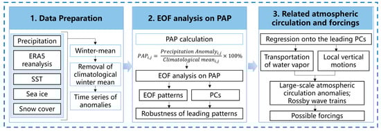
Figure 1.
Flowchart of data and methods used in this study.
3. Results
3.1. Distinct Variations in Winter P in Southern EA and NEA
Figure 2a shows the climatological mean of winter P in EA, characterized by a wetter south and a drier north [10]. Specifically, the wetter areas mainly include southern China, the southern Korean Peninsula, and southern Japan, while the drier areas are mainly found in NEA. Despite less winter P, NEA has a higher chance to experience frozen and freezing rain, since the winter average temperature is likely to fall below zero in this region. It is vital to gain an in-depth understanding of the characteristics and drivers of winter P variability in NEA.
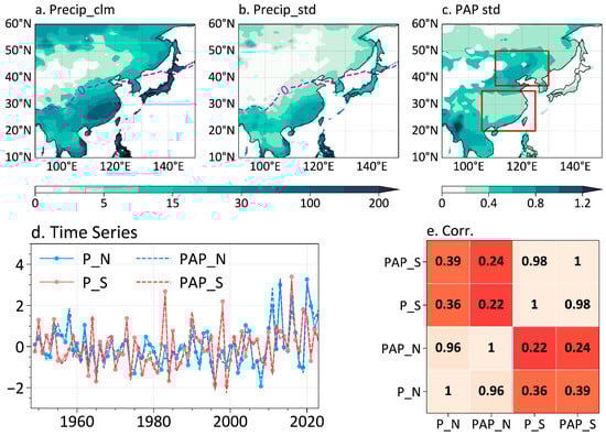
Figure 2.
(a) Winter mean P (mm/month) in EA during 1950–2023; (b) standard deviation of winter P in EA; (c) same as (b), but for PAP; (d) time series of area-mean winter P/PAP (solid/dashed lines) in NEA (in blue) and southern EA (in red); (e) heatmap of c.c. between the four time series in (d), with long-term trends removed. The upper and lower boxes in (c) represent the NEA (37–50° N, 110–130° E) and the southern EA (20–35° N, 115–125° E) regions, respectively. The purple contours in (a,b) indicate the isoline of zero surface air temperature. All the time series in (d) were normalized by their respective standard deviations to ensure comparability.
Figure 2b,c present the standard deviation of winter P and PAP, respectively. The pattern in Figure 2b closely resembles the climatological mean, suggesting that larger variations are associated with higher total precipitation levels. In contrast, Figure 2c shows greater variability in NEA, indicating sharp year-to-year fluctuations in local winter P. In other words, NEA experiences more pronounced fluctuations in winter P compared to the southern regions.
The next question is whether the variations in winter P between NEA and southern EA are coherent or distinct. Figure 2d displays the time series of area-mean P and PAP for both regions (red boxes in Figure 2c). As expected, PAP and P within each region are highly consistent, with a correlation coefficient (c.c.) of 0.96 and 0.98, respectively. However, winter P variations between NEA and southern EA differ notably, as indicated by a low c.c. of 0.24 for PAP. This analysis indicates that winter P in NEA varies differently from that in southern EA, underscoring the necessity for a more in-depth exploration of the former.
Zooming into the NEA region, the evolution of winter temperature and P are displayed in Figure 3. In this region, temperatures drop below zero starting in November and gradually rise again by March. During the winter months (November through February), November experiences the highest precipitation, whereas January sees the lowest (Figure 3g).
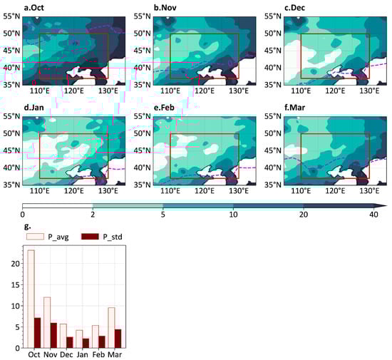
Figure 3.
(a–f) Climatological mean winter P in NEA from October to March, respectively. (g) The area-averaged winter P in NEA (light red bars) along with its standard deviation (dark red bars) for the same period. Red boxes in (a–f) indicate the NEA region. The purple contours in (a–f) indicate the isoline of zero surface air temperature.
3.2. Dominant Modes of Interannual Variability of Winter P in NEA
An EOF analysis was conducted to detect the principle patterns of winter PAP in NEA, as shown in Figure 4. The first EOF mode (EOF1) features a uniform spatial pattern in the NEA region (Figure 4a). The second EOF mode (EOF2) displays a north–south dipole pattern (Figure 4b) while the third EOF mode (EOF3) has a west–east contrasting spatial pattern (Figure 4c). These three EOF modes explain approximately 45.5%, 17.9%, and 7.3% of the overall variability, respectively. Given the EOF1 and EOF2 account for the majority of the variance and meet North’s criteria, we will focus on these two modes in the subsequent analysis. Moreover, this study concentrates on the interannual variability of the corresponding PCs (PC1, PC2, and PC3), although they show low-frequency decadal variations.
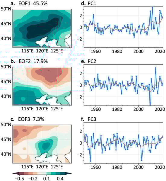
Figure 4.
Results of the EOF analysis on winter PAP in NEA. (a–c) Spatial distributions of the three EOF modes; (d–f) the corresponding PC time series (blue lines) and its decadal component (red dashed lines).
3.3. Atmospheric Circulations Associated with These Dominant Modes
Precipitation anomalies are primarily driven by two key factors: vertical air lifting and the transport of water vapor. These physical variables are analyzed to investigate the direct circulation causes of variations in the first two PCs (Figure 5). PC1 is linked to region-wide vertical ascending motions (Figure 5a). These ascending motions extended from the near surface up to the higher tropospheric layer (Figure 5c). Despite the anomalous southerly transportation of moisture to NEA, the magnitude is relatively small and insignificant (Figure 5e). In contrast, PC2 is connected to ascending and descending in the northern and southern parts of NEA, respectively. This ascent is connected to a notable weakening of the local Hadley cell over East Asia. Overall, this analysis indicates that variations in winter P in NEA are associated with water vapor phase change due to vertical lifting, whereas horizontal water vapor transport may play a less important role.
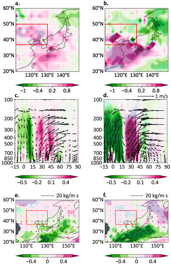
Figure 5.
Atmospheric circulation anomalies regressed onto PC1 (a,c,e) and PC2 (b,d,f). (a,b) 500 hPa vertical velocity (−102 Pa s−1). (c,d) Local Hadley cell averaged along 110–130° E. The black vectors indicate meridional wind (m s−1) and vertical velocity (amplified by a factor of 102, Pa s−1); the legend for these vectors is shown at the top right of (e). (e,f) Water vapor transportation flux (1000–300 hPa, vectors, kg m−1s−1) and its divergence (color, 10−5 kg m−2s−1). Areas with dotting indicate where p-values are ≤0.1, highlighting statistically significant regions. Red boxes in (a, b, e, and f) represent the NEA region (37–50° N, 110–130° E).
Following the identification of in situ atmospheric circulation anomalies, we further explore the large-scale circulation variations associated with the two EOFs, as illustrated in Figure 6 and Figure 7.
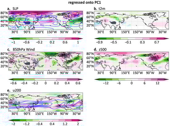
Figure 6.
Regression patterns onto PC1: (a) SLP (color, hPa), (b) T2M (degrees Celsius), (c) horizontal winds at 850 hPa (black vectors, m s−1), with meridional wind colored, (d) 500 hPa geopotential height (Z500, m), and (e) 200 hPa zonal wind (color, m s−1). Areas with dotting indicate where p-values are ≤0.1, highlighting statistically significant regions. In panel (a), the contours represent the climatological mean of winter sea level pressure (SLP), ranging from 1000 hPa to 1030 hPa, with intervals of 5 hPa. In panel (e), the blue contours depict the winter mean of the zonal wind at 200 hPa, with contour levels at 20, 30, 40, 50, and 60 m/s.
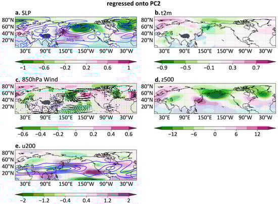
Figure 6 highlights the key atmospheric circulation related to PC1. Both the southeastern edge of the SH and the western edge of the AL are weakened. This reduces the SLP gradient between the SH and AL, resulting in southerly wind anomalies over NEA, that is, a weakened north sub-mode of the EAWM. These southerly wind anomalies facilitate enhanced moisture transport to NEA. A Rossby wave train propagates from Central Siberia towards Japan, leading to a weakened East Asian trough (EAT) [33]. The subtropical westerly jet stream shifts towards the equator [34]. This equatorward shift in the jet stream is linked to anomalous ascending motions around 30° N [35,36], facilitating precipitation. Overall, PC1 is linked to a weakened SH, a weakened western edge of the AL, a diminished northern EAWM, a shallower EAT, and an equatorward-shifted westerly jet.
Figure 7 is the same as Figure 6, but regressed onto PC2. We observe a northeastern-shifted AL, with anomalous high pressure near Japan. Concurrently, anticyclonic flows appear over the EA–Northwest Pacific (NWP) region, facilitating the northward movement of warm, moisture air from the tropical oceans. In the middle of the troposphere, a Western Pacific-like pattern appears [37], linking to the variations in SLP and near surface temperatures. Specifically, the northern cyclonic flow induces cold anomalies near the Okhotsk Sea, while the southern anticyclone flow contributes to warm anomalies over southern China–southern Japan. The core of the EA jet stream weakens, but westerly acceleration occurs to the north of the jet. These jet variations are associate with changes in local meridional circulation (Figure 5d), including a weakened local Hadley cell and weakened Ferry cell [35]. In summary, variations in PC2 are closely linked to a northwestern-shifted AL, a weakened EAWM in both its northern and southern modes, a Western Pacific-like pattern, a diminished westerly jet core, and accelerated westerlies to the north of the jet.
To investigate the Rossby waves that may contribute to variations in PC1 and PC2, we examine the TN wave activity fluxes, as shown in Figure 8. For PC1 (Figure 8a), a Rossby wave train propagates from Central Siberia towards Japan. The cyclonic flow extends over NEA, facilitating the uplift of local air messes. Meanwhile, the anticyclonic flow over Japan weakens the EAT, causing anomalous rising upstream [33]. Thus, the Rossby wave train over northern Eurasia is crucial in influencing PC1. For PC2 (Figure 8b), a stationary Rossby wave train is observed propagating poleward from Japan toward the Bering Sea. This wave train manifests as a Western Pacific-like pattern, which, as illustrated in Figure 7d, was pivotal in shaping PC2. Overall, PC1 and PC2 are related to distinct Rossby wave activities: PC1 is linked to a wave train propagating over northern Eurasia, whereas PC2 is connected to a wave train along the NWP rim.
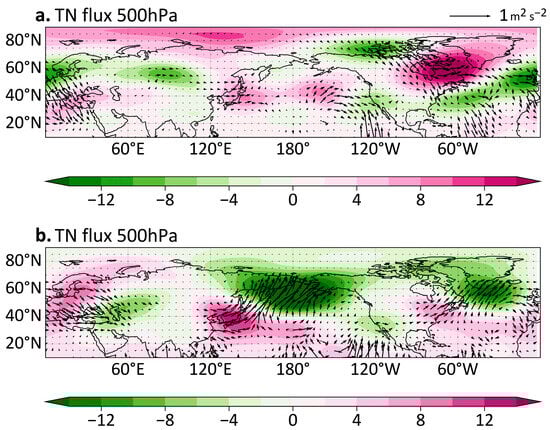
Figure 8.
Regression patterns of 500 hPa TN flux (black vectors, m2 s−2) and geopotential height (color, m) onto (a) PC1 and (b) PC2.
3.4. Possible External Factors Influencing Winter P
Following the identification of atmospheric circulation anomalies, we now examine possible external factors contributing to variations in PC1 and PC2, focusing on anomalies in SST, SIC, and snow depth water equivalent (SDWE).
Figure 9 displays SST anomalies from autumn to winter in relation to the two PCs. For PC1, anomalous cold SSTs appear in the subtropical NWP (Figure 9a). These cold SSTs induce anomalous anticyclonic flows to its northwest (Figure 6c), resulting in anomalous southerly winds over NEA. These cold SST anomalies, established in the previous autumn (Figure 9d), serve as potential indicators for seasonal forecasting.
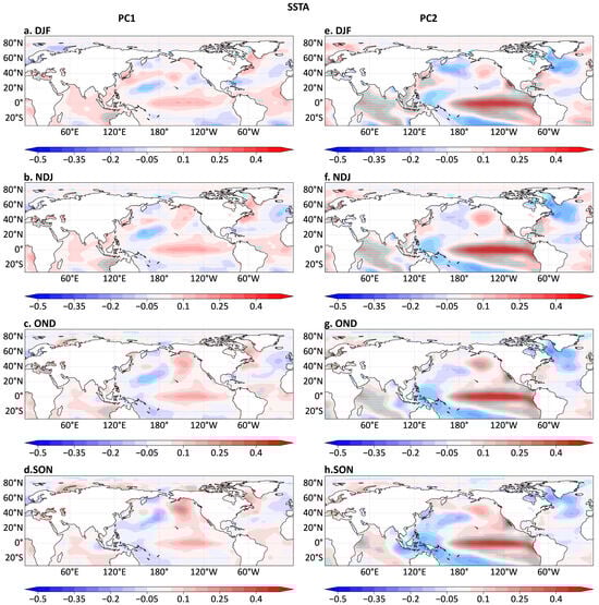
Figure 9.
(a–d) SST anomalies regressed onto PC1 (left column) from the contemporaneous winter (DJF) to the previous autumn (SON). (e–h) as (a–d) but for PC2. Areas with dotting indicate where p-values are ≤0.1, highlighting statistically significant regions.
In the case of PC2, SST anomalies are observed in the tropical Indo-Pacific Ocean. An El Niño-like pattern emerges in autumn and develops during winter. Concurrently, the tropical Indian Ocean exhibits an Indian Ocean Dipple (IOD) mode in autumn, transitioning to an Indian Ocean Basin Warming (IOBW) mode in winter (Figure 9e–h). The combination of warm ENSO and IOBW enhances the anomalous anticyclone over NWP, leading to increased rainfall in southern EA [12,17,38,39]. Notably, cold SST in the tropical western Pacific weakens the local Hadley cell, causing anomalous divergence over subtropical EA in the upper tropospheric level. This divergence acts as Rossby wave sources which act on the jet stream, generating a wave train propagating poleward. Additionally, an upstream wave train, originating from the North Atlantic and propagating along the 21st-century Maritime Silk Road, contributes to the NWP anomalies.
The SIC variations associated with PC1 and PC2 are illustrated in Figure 10. Our analysis focused on early winter (November–December mean) since SIC variations are minimal in late winter months. For PC1, we observe a reduction in SIC in the Barents–Kara Seas (BKS), correlating with warm conditions during autumn (Figure 9d). This reduction in BKS SIC contributes to a warmer Arctic and colder northeastern Eurasia (Figure 6b) [40,41]. Conversely, for PC2, there is an increase in SIC near Baffin Bay.
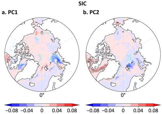
Figure 10.
Regression patterns of Arctic SIC anomalies averaged in November–December on (a) PC1 and (b) PC2. Areas with dotting indicate where p-values are ≤0.1, highlighting statistically significant regions.
Figure 11 illustrates anomalies in SDWE associated with variations in the two leading PCs. PC1 is linked to increased SDWE over central to eastern Eurasia (40–60° N, 80–120° E). This increase tends to lower near surface temperature via heat exchange processes, such as sensible, latent heat fluxes and increased albedo. The resulting local temperature decrease, in turn, helps to maintain the wave train towards Japan. Changes in snow in central Eurasia may serve as potential external factors influencing PC1. In the case of PC2, a decrease in SDWE is observed over Europe. This reduction correlates with the anticyclonic flows over northern Europe (Figure 7d) and tends to amplify warmer temperatures via positive air–land feedback processes. The warm air contributes to the wave train along the 21st-century Maritime Silk Road (Figure 8b).
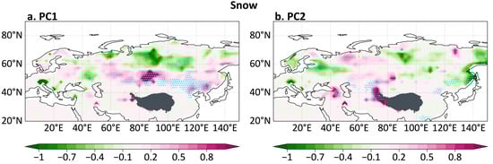
Figure 11.
Regression of snow depth water equivalent anomalies onto (a) PC1 and (b) PC2. Areas with dotting indicate where p-values are ≤0.1, highlighting statistically significant regions.
Chen et al. (2023) [42] explored the mechanism by which autumn snow cover in Central Asia influences winter P in NEA. They found that a reduction in snow warms the atmosphere, leading to the formation of an anomalous anticyclone over Central Asia. This anticyclone, in conjunction with a Rossby wave train originating from the North Atlantic, propagates eastward. This wave train forces an anomalous cyclone over NEA and an anomalous anticyclone over the western North Pacific. The southerly anomalies between them enhance the transport of moist air from the Pacific to the continent, thereby increasing precipitation in NEA.
4. Conclusions and Discussion
This study investigated the interannual variability of winter rainfall in the NEA region (37–50° N, 110–130° E). A comparison analysis showed that winter P variations are distinct between southern EA and NEA regions. Specifically, the c.c. of PAP between these two regions only reaches 0.24 during the analysis period of 1950–2023.
An EOF analysis was performed to detect the NEA PAP variation characteristics. EOF1 and EOF2 explained approximately 63.4% of the total variance. EOF1 has a region-wide uniform pattern of PAP. EOF2 has a north–south opposite PAP pattern. Diagnostic analysis suggested that, for both modes, vertical motion anomalies primarily contributed to the PAP variations, and the water vapor transport played a secondary role.
The two leading modes are linked to different large-scale atmospheric circulation anomalies and possible external forcings.
EOF1 is linked to a Rossby wave train propagating from Central Siberia towards Japan. This wave train weakened the EAT and thus induced an anomalous rising upstream of the trough in the NEA region. Simultaneously, this wave train reduced the pressure gradient between the SH and AL, causing southerly wind anomalies over NEA. The co-occurrence of uplifting and southerly wind anomalies contributed to increased rainfall in the NEA. Further analysis suggested that this wave train may be related to decreased SIC in BKS and increased SDWE over Central Siberia.
The second mode exhibits a strong correlation with SST in the tropical Indo-Pacific Ocean. Cooling in the tropical western Pacific weakens the local EA Hadley circulation, leading to anomalous divergence in the upper layers of subtropical EA. These divergences act as sources of Rossby waves and generate a wave train that manifests as a Western Pacific-like pattern. This anomaly contributes to contrasting PAP in the north and south parts of NEA. Additionally, a Rossby wave train along the 21st-century Maritime Silk Road may also contribute to the Western Pacific-like anomaly.
This study has several limitations. First, the mechanisms by which SST, SIC, and snow influence NEA winter P warrant further investigation using numerical models. Second, the relative contributions of these factors should be quantified in further research. Despite these limitations, this study highlights that winter P in NEA exhibits distinct characteristics compared to southern EA regions. Notably, the first mode is correlated with SST, SIC and snow in the mid-high latitudes while the second mode shows a close relationship with tropical SST.
We conducted a comparative analysis of winter P in NEA and the EAWM. Specifically, Figure 12 presents the c.c. between the area-mean winter P in NEA and seven EAWM indexes defined in previous studies. These indexes capture different aspects of the EAWM system: the Chen2000 [43] and Yang2002 [34] indexes represent variations in the lower-layer meridional wind over EA; the Jhun2024 [44] index reflects zonal wind shear along the westerly jet; the Gong2001 [45] index is based on the strength of the SH; the Chen2014N and Chen2014S [20] indexes indicate 1000 hPa meridional wind variations in northern and southern EA, respectively; and the Sun1997 [46] index measures the intensity of the EAT. Notably, the area-mean winter P in NEA shows significant correlations with all EAWM indexes except Gong2001 [45]. Among these, Yang2002 [34] and Sun1997 [46] exhibit the strongest correlations (both 0.43), suggesting that a weakened EAWM and a shallower-than-normal EAT likely contribute to increased winter P in NEA. Moreover, although the EAWM indexes exhibit significant correlations with winter P, these c.c. values are moderate (less than 0.43), indicating that EAWM is not the sole dominant impact factor.
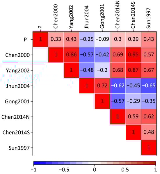
Figure 12.
Correlation between the area-mean winter P in NEA and various EAWM indexes. c.c. values with absolute magnitudes ≥ 0.20 (0.23) exceed the significance thresholds of α = 0.1 (0.05), respectively. The definitions of the indexes are as follows: P: precipitation averaged in the region of NEA (37–50° N, 110–130° E); Chen2000: v-wind at 10 m averaged over the regions of (10–25° N, 110–130° E and 25–40° N, 120–140° E) [43]; Yang2002: v-wind at 850 hPa averaged over the region of (20–40° N, 100–140° E) [34]; Jhun2004: difference in area-mean u-wind at 300 hPa between (27.5–37.5° N, 110–170° E) and (50–60° N, 80–140° E) [44]; Gong2001: sea level pressure averaged over (40–60° N, 70–120° E) [45]; Chen2014N and Chen2014S: v-wind at 1000 hPa averaged over (35–55° N, 110–125° E) and (10–25° N, 105–135° E), respectively [20]; Sun1997: geopotential height at 500 hPa averaged over (30–45° N, 125–145° E) [46].
To assess the sensitivity of the EOF analysis, we expanded the EOF analysis region from NEA (37–50° N, 110–130° E) to a slightly larger area of (32–55° N, 105–135° E). As shown in Figure 13a,b, the spatial patterns of the two leading EOF modes are nearly identical to those in Figure 4a,b, with the c.c. between PCs exceeding 0.99. These results indicate that the EOF result is relatively robust to variations in the analysis region.
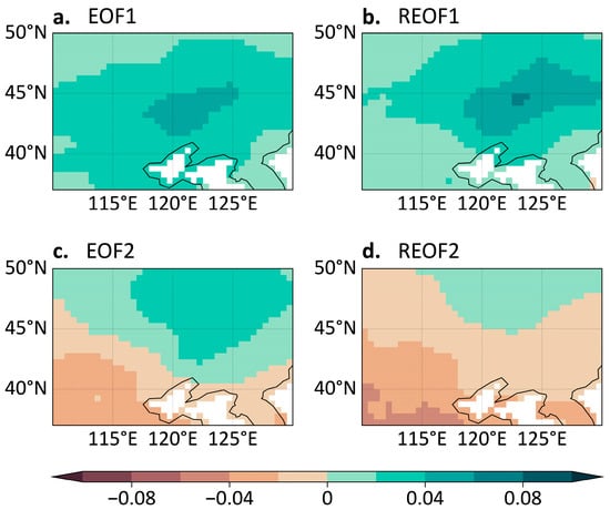
Figure 13.
(a,c) Spatial patterns of the two leading modes of EOF analysis on winter PAP in the area of (32–55° N, 105–135° E); (b,d) the same as (a,c), but with REOF analysis.
We also conducted a rotated EOF (REOF) [47] to evaluate the robustness of the leading patterns derived from the traditional EOF approach [48]. As illustrated in Figure 13a,b, the spatial patterns of the first EOF and the REOF modes closely resemble each other. The c.c. of their respective PC1s is 0.95. For the second mode, both EOF and REOF analysis reveal a north–south dipole pattern, although the dividing line in REOF shifts slightly northward compared to EOF. The c.c. between their PC2s is 0.73. The analysis indicates that the first mode is robust across both EOF and REOF methods, while the second mode exhibits slight differences in spatial patterning. In addition, we compared the EOF results derived from the covariance matrix and the correlation matrix. The spatial patterns of the first two modes and their corresponding PCs are found to be nearly identical, with c.c. values exceeding 0.99.
Additionally, a regression analysis using the EOF-based PCs and an area-mean PAP index was performed for comparison (Figure S1). The PAP index is defined as the area-mean PAP within the NEA region. As illustrated in Figure S1a,b, the regressed spatial patterns based on the PAP index and PC1 are nearly identical. Further calculation reveals a spatial c.c. of 0.99 between the two patterns, conforming a strong similarity. Moreover, as shown in Figure S1a–c, the majority of the regressed coefficients surpass the 0.1 significance threshold. These analyses indicate that the spatial patterns are robust and statistically reliable.
It is noteworthy that winter P in NEA has shown an increasing trend over the past two decades. To access this trend, two additional precipitation datasets were utilized: the Global Precipitation Climatology Project (GPCP) [49] and the Climatic Research Unit (CRU) [50]. The results indicate that both of these datasets consistently present an increasing trend from 2000 to the present. The underlying mechanism driving this trend warrants further research. This rise in precipitation, combined with consistently sub-zero temperatures, may lead to more frequent extreme snowstorms and freezing rain events. Hence, it is crucial to reduce the uncertainty in future projections of winter P in NEA. To address this issue, we need to assess the extent to which variations in winter P are due to anthropogenic external forcings versus natural climate variability. This study contributes to our understanding of winter P associated with internal climate variability.
Supplementary Materials
The following supporting information can be downloaded at: https://www.mdpi.com/article/10.3390/w17020219/s1, Figure S1. Regression patterns of precipitation anomaly percentage (PAP) onto three indexes.
Author Contributions
Conceptualization, T.M. and W.C.; methodology, T.M.; writing—original draft preparation, Y.Z. and T.M.; writing—review and editing, T.M., Y.L. and W.C.; supervision, W.C.; funding acquisition, T.M. and W.C. All authors have read and agreed to the published version of the manuscript.
Funding
This research was funded by the National Natural Science Foundation of China (award number 42475043), the Yunnan Southwest United Graduate School Science and Technology Special Project (award number 202302AP370003), and the Yunnan International Joint Laboratory of Monsoon and Extreme Climate Disasters (award number 202403AP140009).
Data Availability Statement
All data used in this study can be accessed at the following websites: NOAA’s PREC/L: https://psl.noaa.gov/data/gridded/data.precl.html (accessed on 1 January 2024); ECMWF’s ERA5: https://www.ecmwf.int/en/forecasts/dataset/ecmwf-reanalysis-v5 (accessed on 1 January 2024); NOAA ERSST_V5: https://psl.noaa.gov/data/gridded/data.noaa.ersst.v5.html (accessed on 1 January 2024); Met Office Hadley Centre SIC: https://www.metoffice.gov.uk/hadobs/hadisst/ (accessed on 1 January 2024); and ERA5-land SDWE: https://cds.climate.copernicus.eu/datasets/reanalysis-era5-land-monthly-means (accessed on 1 January 2024). Codes used to generate all the figures in this paper can be obtained by contacting the corresponding author.
Acknowledgments
We sincerely thank the editors and anonymous reviewers for their constructive comments and valuable suggestions.
Conflicts of Interest
The authors declare no conflicts of interest.
References
- Sun, C.H.; Yang, S. Persistent Severe Drought in Southern China during Winter-Spring 2011: Large-Scale Circulation Patterns and Possible Impacting Factors. J. Geophys. Res.-Atmos. 2012, 117, D10112. [Google Scholar] [CrossRef]
- You, Q.; Jiang, Z.; Yue, X.; Guo, W.; Liu, Y.; Cao, J.; Li, W.; Wu, F.; Cai, Z.; Zhu, H.; et al. Recent Frontiers of Climate Changes in East Asia at Global Warming of 1.5 °C and 2 °C. Npj Clim. Atmos. Sci. 2022, 5, 1–17. [Google Scholar] [CrossRef]
- Chen, W.; Zhang, R.; Wu, R.; Wen, Z.; Zhou, L.; Wang, L.; Hu, P.; Ma, T.; Piao, J.; Song, L.; et al. Recent Advances in Understanding Multi-Scale Climate Variability of the Asian Monsoon. Adv. Atmos. Sci. 2023, 40, 1429–1456. [Google Scholar] [CrossRef]
- Tao, S.; Wei, J. Severe Snow and Freezing-Rain in January 2008 in the Southern China. Clim. Environ. Res. 2008, 13, 337–350. [Google Scholar]
- Zong, H.F.; Bueh, C.; Peng, J.B. Combined Disaster Events of Extensive and Persistent Low Temperatures, Rain/Snow, and Freezing in Southern China: Objective Identification and Key Features. Chin. J. Atmos. Sci. Chin. 2022, 46, 1055–1070. [Google Scholar] [CrossRef]
- Zhou, B.; Gu, L.; Ding, Y.; Shao, L.; Wu, Z.; Yang, X.; Li, C.; Li, Z.; Wang, X.; Cao, Y.; et al. The Great 2008 Chinese Ice Storm: Its Socioeconomic–Ecological Impact and Sustainability Lessons Learned. Bull. Am. Meteorol. Soc. 2011, 92, 47–60. [Google Scholar] [CrossRef]
- Zhou, L.-T.; Wu, R. Respective Impacts of the East Asian Winter Monsoon and ENSO on Winter Rainfall in China. J. Geophys. Res. Atmos. 2010, 115, D02107. [Google Scholar] [CrossRef]
- Ma, T.; Chen, W.; Feng, J.; Wu, R. Modulation Effects of the East Asian Winter Monsoon on El Nino-Related Rainfall Anomalies in Southeastern China. Sci. Rep. 2018, 8, 14107. [Google Scholar] [CrossRef]
- Zhou, L.T. Impact of East Asian Winter Monsoon on Rainfall over Southeastern China and Its Dynamical Process. Int. J. Clim. 2011, 31, 677–686. [Google Scholar] [CrossRef]
- Wang, L.; Feng, J. Two Major Modes of the Wintertime Precipitation over China. Chin. J. Atmos. Sci. 2011, 35, 1105–1116. (In Chinese) [Google Scholar]
- Qian, Q.; Jia, X. Seasonal Forecast of Winter Precipitation over China Using Machine Learning Models. Atmos. Res. 2023, 294, 106961. [Google Scholar] [CrossRef]
- Zhang, R.; Sumi, A.; Kimoto, M. Impact of El Nino on the East Asian Monsoon: A Diagnostic Study of the ’86/87 and ’91/92 Events. J. Meteorol. Soc. Jpn. 1996, 74, 49–62. [Google Scholar] [CrossRef]
- Zhang, R.; Min, Q.; Su, J. Impact of El Niño on Atmospheric Circulations over East Asia and Rainfall in China: Role of the Anomalous Western North Pacific Anticyclone. Sci. China Earth Sci. 2017, 60, 1124–1132. [Google Scholar] [CrossRef]
- Jia, X.; Ge, J.; Wang, S. Diverse Impacts of ENSO on Wintertime Rainfall over the Maritime Continent. Int. J. Climatol. 2016, 36, 3384–3397. [Google Scholar] [CrossRef]
- Wang, B.; Wu, R.G.; Fu, X.H. Pacific-East Asian Teleconnection: How Does ENSO Affect East Asian Climate? J. Clim. 2000, 13, 1517–1536. [Google Scholar] [CrossRef]
- Wu, R.G.; Hu, Z.Z.; Kirtman, B.P. Evolution of ENSO-Related Rainfall Anomalies in East Asia. J. Clim. 2003, 16, 3742–3758. [Google Scholar] [CrossRef]
- Ashok, K.; Guan, Z.Y.; Saji, N.H.; Yamagata, T. Individual and Combined Influences of ENSO and the Indian Ocean Dipole on the Indian Summer Monsoon. J. Clim. 2004, 17, 3141–3155. [Google Scholar] [CrossRef]
- Zhu, L.; Wu, Z. Climatic Influence of the Antarctic Ozone Hole on the East Asian Winter Precipitation. Npj Clim. Atmos. Sci. 2024, 7, 184. [Google Scholar] [CrossRef]
- Wang, B.; Wu, Z.W.; Chang, C.P.; Liu, J.; Li, J.P.; Zhou, T.J. Another Look at Interannual-to-Interdecadal Variations of the East Asian Winter Monsoon: The Northern and Southern Temperature Modes. J. Clim. 2010, 23, 1495–1512. [Google Scholar] [CrossRef]
- Chen, Z.; Wu, R.; Chen, W. Distinguishing Interannual Variations of the Northern and Southern Modes of the East Asian Winter Monsoon. J. Clim. 2014, 27, 835–851. [Google Scholar] [CrossRef]
- Chen, Z.; Wu, R.; Chen, W. Impacts of Autumn Arctic Sea Ice Concentration Changes on the East Asian Winter Monsoon Variability. J. Clim. 2014, 27, 5433–5450. [Google Scholar] [CrossRef]
- North, G.R.; Bell, T.L.; Cahalan, R.F.; Moeng, F.J. Sampling Errors in the Estimation of Empirical Orthogonal Functions. Mon. Weather Rev. 1982, 110, 699–706. [Google Scholar] [CrossRef]
- Nie, Y.; Sun, J. Causes of Interannual Variability of Summer Precipitation Intraseasonal Oscillation Intensity over Southwest China. J. Clim. 2022, 35, 3705–3723. [Google Scholar] [CrossRef]
- Goswami, B.N.; Mohan, R.S.A. Intraseasonal Oscillations and Interannual Variability of the Indian Summer Monsoon. J. Clim. 2001, 14, 1180–1198. [Google Scholar] [CrossRef]
- Chen, M.Y.; Xie, P.P.; Janowiak, J.E.; Arkin, P.A. Global Land Precipitation: A 50-Yr Monthly Analysis Based on Gauge Observations. J. Hydrometeorol. 2002, 3, 249–266. [Google Scholar] [CrossRef]
- Hersbach, H.; Bell, B.; Berrisford, P.; Hirahara, S.; Horányi, A.; Muñoz-Sabater, J.; Nicolas, J.; Peubey, C.; Radu, R.; Schepers, D.; et al. The ERA5 Global Reanalysis. Q. J. R. Meteorol. Soc. 2020, 146, 1999–2049. [Google Scholar] [CrossRef]
- Huang, B.; Thorne, P.W.; Banzon, V.F.; Boyer, T.; Chepurin, G.; Lawrimore, J.H.; Menne, M.J.; Smith, T.M.; Vose, R.S.; Zhang, H.-M. Extended Reconstructed Sea Surface Temperature, Version 5 (ERSSTv5): Upgrades, Validations, and Intercomparisons. J. Clim. 2017, 30, 8179–8205. [Google Scholar] [CrossRef]
- Rayner, N.A.; Parker, D.E.; Horton, E.B.; Folland, C.K.; Alexander, L.V.; Rowell, D.P.; Kent, E.C.; Kaplan, A. Global Analyses of Sea Surface Temperature, Sea Ice, and Night Marine Air Temperature since the Late Nineteenth Century. J. Geophys. Res.-Atmos. 2003, 108, 4407. [Google Scholar] [CrossRef]
- Muñoz Sabater, J. ERA5-Land Monthly Averaged Data from 1950 to Present 2019. Available online: https://cds.climate.copernicus.eu/datasets/reanalysis-era5-land-monthly-means?tab=download (accessed on 1 January 2024).
- Dawson, A. Eofs: Version 1.1.0. 2016. Available online: https://zenodo.org/records/46871 (accessed on 1 January 2024).
- Brown, D.; Brownrigg, R.; Haley, M.; Huang, W. NCAR Command Language (NCL) Version: 6.6.2. 2012. Available online: https://www.ncl.ucar.edu/ (accessed on 1 January 2024).
- Takaya, K.; Nakamura, H. A Formulation of a Phase-Independent Wave-Activity Flux for Stationary and Migratory Quasigeostrophic Eddies on a Zonally Varying Basic Flow. J. Atmos. Sci. 2001, 58, 608–627. [Google Scholar] [CrossRef]
- Song, L.; Wang, L.; Chen, W.; Zhang, Y. Intraseasonal Variation of the Strength of the East Asian Trough and Its Climatic Impacts in Boreal Winter. J. Clim. 2016, 29, 2557–2577. [Google Scholar] [CrossRef]
- Yang, S.; Lau, K.M.; Kim, K.M. Variations of the East Asian Jet Stream and Asian-Pacific-American Winter Climate Anomalies. J. Clim. 2002, 15, 306–325. [Google Scholar] [CrossRef]
- Chan, D.; Zhang, Y.; Wu, Q.; Dai, X. Quantifying the Dynamics of the Interannual Variabilities of the Wintertime East Asian Jet Core. Clim. Dyn. 2020, 54, 2447–2463. [Google Scholar] [CrossRef]
- Wei, W.; Ren, Q.; Lu, M.; Yang, S. Zonal Extension of the Middle East Jet Stream and Its Influence on the Asian Monsoon. J. Clim. 2022, 35, 4741–4751. [Google Scholar] [CrossRef]
- Aru, H.; Chen, S.; Chen, W. Comparisons of the Different Definitions of the Western Pacific Pattern and Associated Winter Climate Anomalies in Eurasia and North America. Int. J. Climatol. 2021, 41, 2840–2859. [Google Scholar] [CrossRef]
- Watanabe, M.; Jin, F.F. A Moist Linear Baroclinic Model: Coupled Dynamical-Convective Response to El Nino. J. Clim. 2003, 16, 1121–1139. [Google Scholar] [CrossRef]
- Ma, T.J.; Chen, W.; Chen, S.F.; Garfinkel, C.I.; Ding, S.Y.; Song, L.; Li, Z.B.; Tang, Y.L.; Huangfu, J.L.; Gong, H.N.; et al. Different ENSO Teleconnections over East Asia in Early and Late Winter: Role of Precipitation Anomalies in the Tropical Indian Ocean and Far Western Pacific. J. Clim. 2022, 35, 4319–4335. [Google Scholar] [CrossRef]
- Hong, Y.; Wang, S.-Y.S.; Son, S.-W.; Jeong, J.-H.; Kim, S.-W.; Kim, B.; Kim, H.; Yoon, J.-H. Arctic-Associated Increased Fluctuations of Midlatitude Winter Temperature in the 1.5° and 2.0° Warmer World. Npj Clim. Atmos. Sci. 2023, 6, 26. [Google Scholar] [CrossRef]
- An, X.; Chen, W.; Sheng, L.; Li, C.; Ma, T. Synergistic Effect of El Niño and Arctic Sea-Ice Increment on Wintertime Northeast Asian Anomalous Anticyclone and Its Corresponding PM 2.5 Pollution. J. Geophys. Res.-Atmos. 2023, 128, e2022JD037840. [Google Scholar] [CrossRef]
- Chen, X.; Jia, X.; Wu, R. Impacts of Autumn-Winter Central Asian Snow Cover on the Interannual Variation in Northeast Asian Winter Precipitation. Atmos. Res. 2023, 286, 106669. [Google Scholar] [CrossRef]
- Chen, W.; Hans-F, G.; Huang, R. The Interannual Variability of East Asian Winter Monsoon and Its Relation to the Summer Monsoon. Adv. Atmos. Sci. 2000, 17, 48–60. [Google Scholar] [CrossRef]
- Jhun, J.G.; Lee, E.J. A New East Asian Winter Monsoon Index and Associated Characteristics of the Winter Monsoon. J. Clim. 2004, 17, 711–726. [Google Scholar] [CrossRef]
- Gong, D.Y.; Wang, S.W.; Zhu, J.H. East Asian Winter Monsoon and Arctic Oscillation. Geophys. Res. Lett. 2001, 28, 2073–2076. [Google Scholar] [CrossRef]
- Sun, B.M.; Li, C.Y. Relationship between the Disturbances of East Asian Trough and Tropical Convective Activities in Boreal Winter. Chin Sci Bull 1997, 42, 500–504. [Google Scholar]
- Richman, M.B. Rotation of Principal Components. J. Climatol. 1986, 6, 293–335. [Google Scholar] [CrossRef]
- Dommenget, D.; Latif, M. A Cautionary Note on the Interpretation of EOFs. J. Clim. 2002, 15, 216–225. [Google Scholar] [CrossRef]
- Adler, R.F.; Huffman, G.J.; Chang, A.; Ferraro, R.; Xie, P.-P.; Janowiak, J.; Rudolf, B.; Schneider, U.; Curtis, S.; Bolvin, D.; et al. The Version-2 Global Precipitation Climatology Project (GPCP) Monthly Precipitation Analysis (1979–Present). J. Hydrometeorol. 2003, 4, 1147–1167. [Google Scholar] [CrossRef]
- Harris, I.; Osborn, T.J.; Jones, P.; Lister, D. Version 4 of the CRU TS Monthly High-Resolution Gridded Multivariate Climate Dataset. Sci. Data 2020, 7, 109. [Google Scholar] [CrossRef] [PubMed]
Disclaimer/Publisher’s Note: The statements, opinions and data contained in all publications are solely those of the individual author(s) and contributor(s) and not of MDPI and/or the editor(s). MDPI and/or the editor(s) disclaim responsibility for any injury to people or property resulting from any ideas, methods, instructions or products referred to in the content. |
© 2025 by the authors. Licensee MDPI, Basel, Switzerland. This article is an open access article distributed under the terms and conditions of the Creative Commons Attribution (CC BY) license (https://creativecommons.org/licenses/by/4.0/).