Three-Dimensional Particle Tracking Velocimetry Investigation of Flow Dynamics Around Simplified Stones at Low Submergence: Implications for Instream Habitat

Abstract

Shallow waterways such as rapids, tributaries and smaller streams can have important ecological functions in both free-flowing and regulated rivers. As more intermittent renewable energy is introduced to the energy system to reduce CO₂ emissions, the operational conditions of hydropower plants are changing. This implies various flow scenarios that can lead to more locations with shallow depths and larger variations in water levels and velocities, resulting in increased impact on the riverine ecosystem. Accurate predictions of these impacts require an understanding of the flow dynamics near large roughness elements such as boulders or trees in shallow river regions. This study uniquely investigates the effect of relative submergence, i.e., water depth relative to boulder size, on the flow field, turbulence, and potential fish habitats around idealized stone shapes (hemispheres) in shallow open channel flow using time-resolved 3D particle tracking velocimetry. The results indicate that varying relative submergence significantly affects recirculation zones, velocity and vorticity distribution, as well as turbulent kinetic energy. Notably, larger regions of lower velocity downstream of the roughness elements were generated at lower submergences, which might be favorable for fish energy conservation. Valuable insights into ecohydraulic engineering and habitat restoration in shallow waterways can be gained by understanding the fundamental flow mechanisms at low submergence for the flow around large roughness elements.

1. Introduction

To reduce CO₂ emissions from electricity production, more intermittent renewable energy sources, such as wind and solar, are introduced into the energy system. Hydropower is currently the largest source of renewable energy in the world [1] and has provided a base load generation of electricity and regulatory capacity for over 100 years. Changes in the operating conditions of hydropower plants are expected to account for the weather-dependent changes in electricity production due to the larger involvement of intermittent sources. In future energy systems, hydropower will adopt a much bigger regulatory role due to its capacity to balance the frequency in the system [2]. This is anticipated to result in more frequent starts and stops in the operating conditions, increased damage to the riverine ecosystem, and an increase in flow alternations, commonly known as hydropeaking. Hydropeaking has been shown to significantly affect the ecosystem downstream of the power plants by altering the spawning behavior of Atlantic salmon Salmo salar and brown trout (Salmo trutta) [3]. Dewatering of spawning areas during low flows can lead to the stranding of juvenile brown trout [4] and may lead to increased mortality of Atlantic salmon eggs [5].

According to the European Union’s Water Framework Directive, all waterbodies in the EU should reach good ecological status. Therefore, it is important to be able to predict the ecological effects of hydropower using hydraulic modeling tools. This includes evaluating minimum mandatory spilling to avoid complete freezing, as well as designing habitats, passages, and spawning areas for fish. In the regulated and free-flowing rivers, it often occurs in areas in the river with shallow water depths, i.e., the water depth is at a comparable length scale to the largest bed structures present. Therefore, it is of interest to understand how the flow field is affected by relatively large roughness elements, e.g., boulders. Currently, hydraulic models based on two-dimensional depth-averaged models employ empirical correlations, such as the Manning coefficient, to describe flow resistance caused by irregularities at the riverbed. The coefficient is typically calibrated against field measurements, to replicate the water depth [6]. The Manning coefficient considers the size of the bed structure, vegetation, and other riverbed irregularities, and is a good representation of flow resistance for large water depths, i.e., when the water depth is significantly larger than the bed structure. However, this way of representing the flow resistance is inadequate when the water depth is shallow, i.e., when the water depth is similar to or lower than the bed structure, e.g., in rapids, bypass channels, and tributaries [7]. This leads to inaccurate predictions of water depth and local flow properties by 2D models. Three-dimensional models, usually based on the Reynolds-Averaged Navier–Stokes (RANS) equations and including a turbulence closure model, are better at capturing the complex fluid flow that occurs in rivers. These types of models are beneficial as they capture 3D effects, such as turbulence, and account for the riverbed’s irregular shape, which significantly influences the flow resistance, especially in shallow waterways. However, 3D models are much more computationally expensive than 2D models, so reduced models that can reliably predict flow resistance under shallow conditions with the presence of large boulders are of great interest to the hydropower industry and the ecohydraulic society.

Many experimental studies have investigated the flow field around large roughness elements. For example, Dey et al. [8] investigated the flow field around a sphere mounted on a rough bed in laboratory experiments using Acoustic Doppler Velocimetry (ADV). They revealed the velocity profile’s streamwise transformation, indicating a strong reversed flow behind the sphere with high turbulence. This was also demonstrated by Tu et al. [9], who used time-resolved Tomographic Particle Image Velocimetry (TPIV) to study the near wake of a hemisphere mounted on a smooth wall. Different spacing between two inline-mounted hemispheres has also been investigated using ADV and was shown to be a vital parameter that influences turbulence characteristics [10]. They also observed negative mean velocity values close to the bottom for closely spaced hemispheres, indicating a recirculation zone between them. Additionally, an increase in relative spacing reduced the length of the recirculation zone. Boulder clusters have been pointed out to significantly contribute to fish habitats [11] since they create essential flow structures, such as the reversal flow with the formation of a wake in the vicinity of the boulder.

The relative submergence (RS) of boulders, defined as the ratio between the water depth and the height of the boulder, has been shown to have a significant effect on the flow field both up- and downstream of the boulder. Laboratory studies of the flow around hemispheres, cylinders, cubes, and natural boulders for a wide range of different submergences have been extensively conducted [12,13,14,15]. Using yaw and pitch probes, the flow field around a hemisphere was classified into different regimes depending on their RS [12], with the RS in the range from 0.66 to 4.27. The work showed that for an RS between 1.3 and 4, surface waves started to appear and that the shear layer from the hemisphere caused mixing throughout the whole depth for an RS between 1 and 1.3. ADV measurements downstream of a standing cylinder revealed similarities in the wake structures between an RS of 1.1 and 2 [13], but showed differences in the vertical flows and the length of the structures in the wake. A depth dependency of the drag coefficient was observed for both a cube and a hemisphere on a rough bed, with the RS varying between 5 and 10, measured both with Laser Doppler Anemometry (LDA) and a drag force sensor [14]. Golpira et al. [15] used Particle Image Velocimetry (PIV) to examine the impacts of RS on the wake flow for a single natural boulder in a boulder array, with the RS ranging between 1.3 and 3. Shamloo et al. [12] revealed similarities in flow structures for higher RS and a notable difference for the lowest, e.g., a 23% decrease in mean recirculation length. In flume experiments, using a natural bed and low RS, the deposition of coarse sediment particles was observed upstream of a hemispherical obstacle. The grain size distribution downstream of the obstacle showed almost no difference in grain size due to the area being mainly controlled by a recirculation zone [16].

A common measure of the suitability of a fish habitat is water velocity. Instream boulders produce low-velocity and recirculation zones, which fish frequently use to conserve energy [17], and create habitats that are advantageous for aquatic species [11]. Variations in turbulence levels, governed by the structure size and shape, are important factors for fish behavior [18] and high levels of turbulence are known to have a substantial impact on their swimming performance.

Several laboratory studies have investigated fish locomotion and behavior under various hydraulic conditions. Reynolds stresses may affect fish swimming and positioning [18]. A study conducted by Silva et al. [19] investigated the impact of various turbulent parameters on fish swimming behavior. The study found that fish tend to favor areas with lower Reynolds Shear Stress (RSS) levels. Turbulent Kinetic Energy (TKE), not average velocity, is the measure of habitat complexity that correlates with Rainbow trout (Oncorhynchus mykiss) abundance, according to a study conducted by Smith et al. [20]. Rainbow trout are attracted to periodic flow structures behind a cylinder due to their experienced reduction in energy expenditure [21]. According to Enders et al. [22,23], juvenile Atlantic salmon experience higher swimming expenses as Turbulent Intensity (TI) increases at a given mean flow velocity. Simmons et al. [24] observed an increase in swimming speed with increasing body length for higher levels of TKE and low levels of TI for Atlantic salmon kelt. On the other hand, according to a study by Liao et al. [25], fish in turbulent environments showed reduced energy expenditure as they used regular vortices to enhance locomotion. However, energy expenditure increases when vortices are irregular and unpredictable [18]. Vorticity is proposed by Crowder et al. [26] as a metric for quantifying flow complexity. Additionally, studies have shown that fish tend to choose areas with small eddies. When encountering eddies of similar size to their body length, they experience disorientation and loss of stability, leading to high energy expenditure [17,19,27]. Link et al. [27] demonstrated the fish Strouhal number, $S{t}_{\mathrm{fish}}$, to be a reliable indicator of fish propulsion. The fish Strouhal number is defined based on tail beat kinematics and swimming speed as $S{t}_{\mathrm{fish}}=f_{TB}\lambda /U$, where $f_{TB}$ is the average tail beat frequency, $\lambda$ is the tail beat amplitude, and U is the swimming speed. This Strouhal number serves as an indicator of propulsion effort, with values typically associated with efficient swimming falling in the range of 0.25 to 0.35. When designing habitats, it can be useful to relate the eddy size created by in-stream obstacles to the length of the fish using the Strouhal number. Depending on the intensity, periodicity, vortex orientation, and scale factors of turbulence, it can either attract or repel fish, facilitating or obstructing their migratory movements [18]. The Turbulence Attraction and Avoidance (TAA) hypothesis [28] acknowledges that fish, like all organisms, perceive their environment at their scales and conditionally, depending on their past exposure history. This leads to a new understanding of turbulence, habitat complexity, and fish habitat occupancy.

Previous research on large boulder-like obstacles at different RS has mainly utilized point or planar measurement techniques, i.e., ADV and 2D PIV, which do not capture the full three-dimensional flow structures. Using a volumetric measurement technique, time-resolved 3D particle tracking velocimetry (PTV), the aim here is to evaluate how the three-dimensional flow field around an idealized stone, represented as a hemisphere, is affected by the change in RS. Time-resolved 3D measurements will provide comprehensive insight into transient three-dimensional flow dynamics by capturing the evolution of flow features over time. The primary objectives are as follows: (1) evaluate the flow field in terms of flow characteristics and turbulent parameters, (2) couple the changes in the flow field to fish preferences and habitats, and (3) provide useful data for calibration of hydraulic modeling tools.

2. Methods

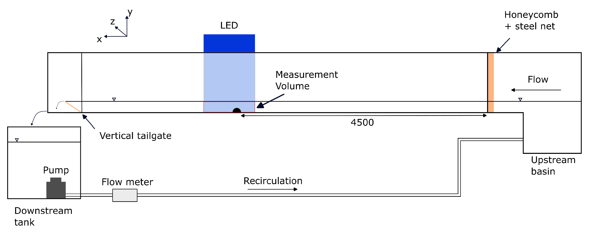
Experiments were carried out in a recirculating open-channel flume in the John Field Laboratory at Luleå University of Technology. The flume, shown in Figure 1, is 7.5 m long, 0.3 m wide, and 0.3 m high. It provides optical access through the side walls and has an adjustable slope. A pump located in a downstream tank is used to recirculate the water while the flow rate is controlled through a KROHNE OPTIFLUX electromagnetic flow meter with an accuracy of ±0.7%.

A flow straightener was used to homogenize the flow entering the flume, consisting of a honeycomb with a thickness of 60 mm and a hole diameter of 6 mm, and a steel net with 2.5 mm × 2.5 mm square holes. The flow depth, h, was controlled through a vertical gate at the flume outlet, and measured with a point gauge. Hemispheres with a radius R = 37.5 mm were mounted along the centerline of the flume; for the single hemisphere case, it was located at a distance of 4.5 m downstream of the inlet to minimize inlet disturbances. In the case with double hemispheres, the second hemisphere was positioned upstream at a center-to-center distance of 4R from the first hemisphere. The distance was selected to create interference between the wake of the upstream hemisphere and the downstream hemisphere [10]. The origin of the Cartesian coordinate system is defined as the center of the single hemisphere, where x, y, and z denote the streamwise, vertical, and spanwise directions, respectively. The flow field may have been impacted by the limited flume width (0.3 m), as the proximity of the sidewalls to the hemispheres could induce unintended effects on the flow. This limitation is recognized and taken into account while analyzing the findings.

Experiments were carried out with a constant slope of 0.005 and a fixed flow rate of 4 L/s, for two different RS, h/R = 1.5 and h/R = 2. The bulk velocity $U_{bulk}$ calculated from the flow rate and the cross-sectional area was 0.23 m/s and 0.18 m/s for h/R = 1.5 and h/R = 2, respectively. The Reynolds number based on the radius, ($R{e}_R=U_{bulk}R/\nu$), varied between 6670 and 8930. The Reynolds number for the open channel flow, ($R{e}_{R_h}=4U_{bulk}{R}_h/\nu$), based on the hydraulic radius, varied between 35,858 and 37,665, and the Froude number, ($Fr=U_{bulk}/\sqrt{gh}$), based on the flow depth, ranged from 0.24 to 0.28.

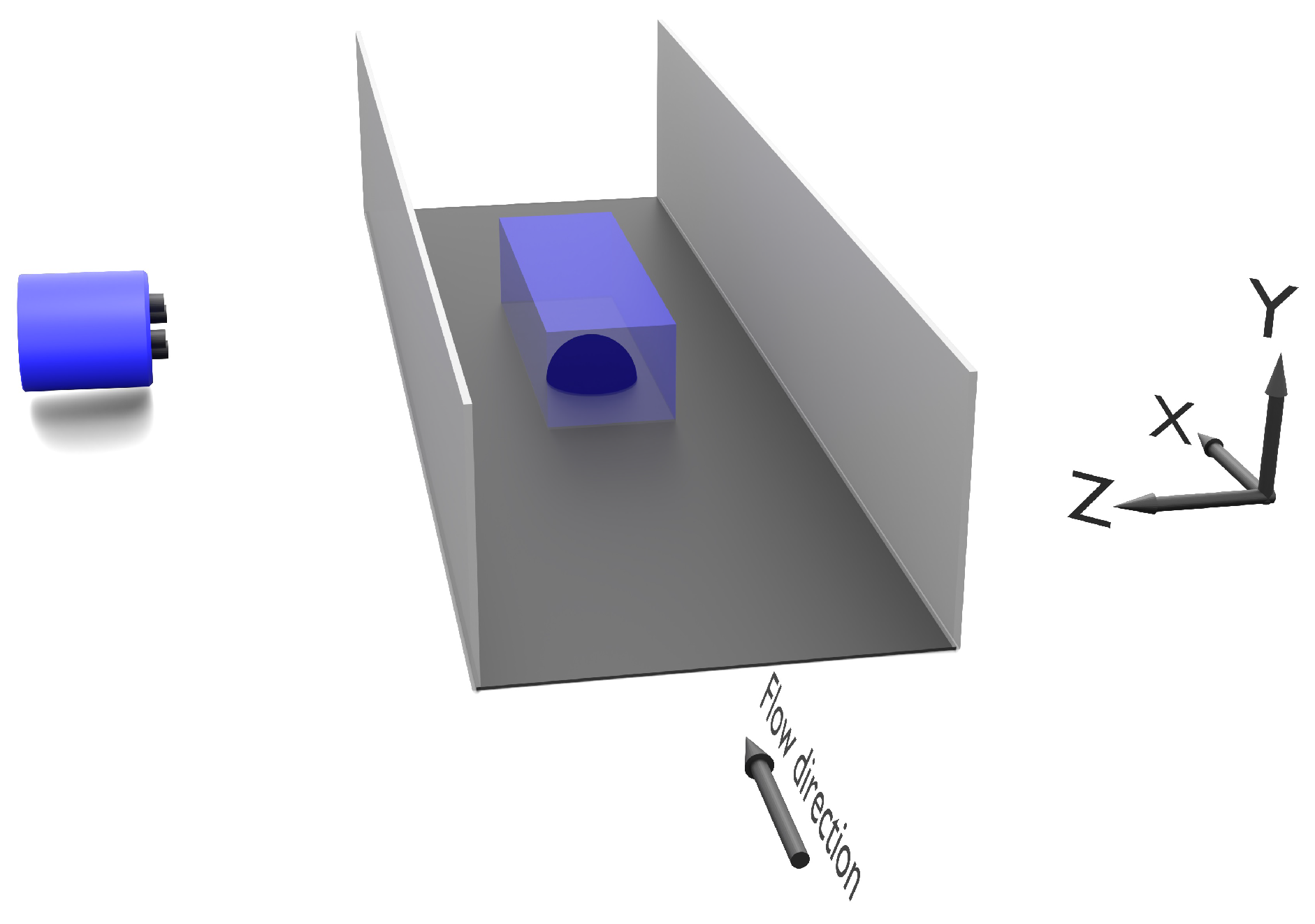
The measurements were carried out with the commercially available time-resolved 3D PTV system, MiniShaker Aero, from LaVision GmbH. The system consists of an aerodynamical camera housing containing four CMOS cameras (2.5 MP, 10 bit, 4.8 × 4.8 μm pixel size), a pulsed LED panel (LED-Flashlight 300 blue, LaVision GmbH, Göttingen, Germany, peak emission wavelength: 450 nm) for volumetric illumination of the flow field and the software DaVis 10.2.0. Triggering and synchronization of the cameras and the LED were assured by a programmable timing unit (PTU X from LaVision GmbH). A UR5e robotic arm from Universal Robots Inc. was used to control the position of the cameras. The flow was seeded with fluorescent particles made of polyethylene (diameter between 125 and 150 μm and a density of 1 g/cm³) with a peak emission wavelength of 606 nm. Every camera was equipped with an 8 mm Fujinon lens with aperture $f_{\#}$ = 8 and a long pass filter for fluorescent light removing disturbing light with a wavelength below 540 nm.

To ensure high-quality results, the camera calibration was performed in two steps. First, a planar calibration target was traversed in the cameras’ line of sight between z = −50 and z = 50 mm. Pictures were acquired in six positions by all four cameras and a mapping between images and physical space was calculated with a fit error of 0.09 pixels and a scale factor of 4.19 mm/pixel. To improve the mapping and reduce the disparity, volume self-calibration [29] was applied, resulting in an average disparity of 0.03 voxels and a maximum disparity of 0.09 voxel.

Images were acquired in a measurement volume for the single case starting at x = −65 mm and for the double case starting at x = −112.5 mm, with a size of 300 × 75 × 100 mm³, and at a camera working distance of 400 mm from the centerline of the flume, shown in Figure 2. In total, 4000 single-frame images were captured at 150 Hz and 200 Hz for the higher and lower RS, respectively. The acquisition rates were selected to ensure similar particle displacement. The average seeding density was approximately 0.01 particles per pixel.

To eliminate background noise, the acquired images were preprocessed with a time filter which subtracts the minimum value for each pixel for the full range of images. Image noise was reduced by applying a spatial filter that operates with a 4 × 4 pixel sliding window, which subtracts the minimum intensity. Normalization of the particle intensity to the first frame was performed and smoothed locally across a window of 200 × 200 pixels. The particle images were processed with the Shake-the-Box algorithm [30] implemented in DaVis to obtain Lagrangian particle tracks. The velocity data from the particle tracks were converted to an Eulerian grid using the Fine Scale Reconstruction (FSR) algorithm combined with the data assimilation technique VIC# [31] to facilitate the visualization of the data. The FSR was performed over 100 iterations with the VIC# denoising factor at 0.001. A summary of parameters obtained in the volume reconstruction is presented in

Table 1. Summary of parameters for the volume data reconstruction.

Case	Particles in Volume	Avg. Track Length Time Steps	Final Volume Vectors	Final Volume mm3
Single High	1478	25	76 × 27 × 39	197 × 68 × 100
Single Low	852	14	76 × 17 × 39	195 × 44 × 100
Double High behind	1383	24	62 × 26 × 42	151 × 62 × 100
Double Low behind	813	21	64 × 18 × 42	151 × 40 × 100
Double High front	657	18	30 × 24 × 39	73 × 62 × 100
Double Low front	368	15	32 × 18 × 42	73 × 40 × 100

, where low and high refer to h/R = 1.5 and 2, respectively. The average uncertainty for the streamwise velocity in the reconstructed volumes behind the hemispheres is estimated by ${ϵ}_u=\langle {\sigma }_u\rangle /\sqrt{N_s}\approx 0.005$ m/s, where ${\sigma }_u$ and $N_s$ is the standard deviation of the streamwise velocity component and the number of samples, respectively.

3. Results

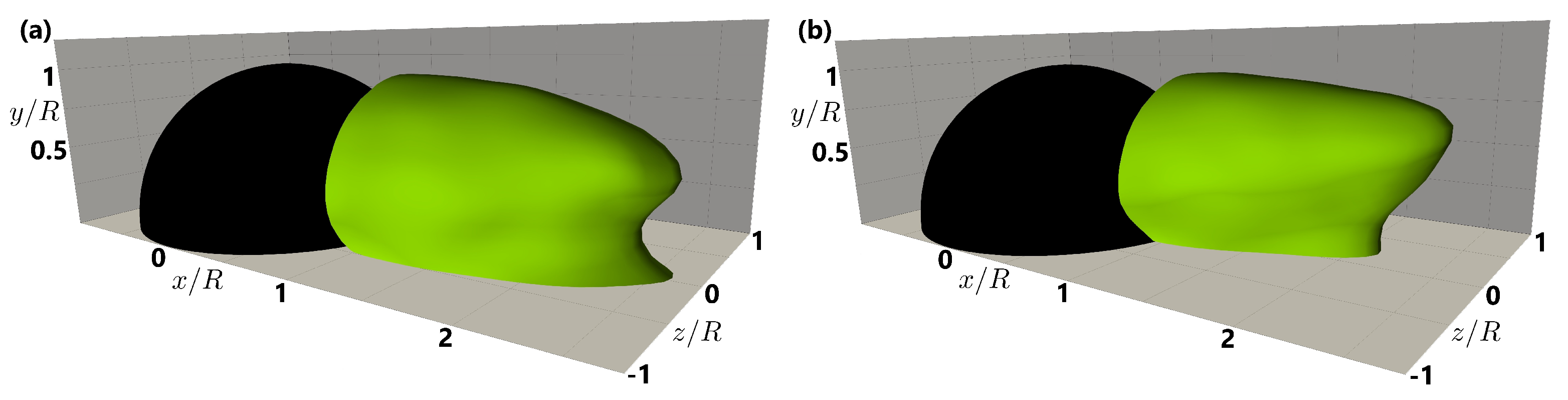
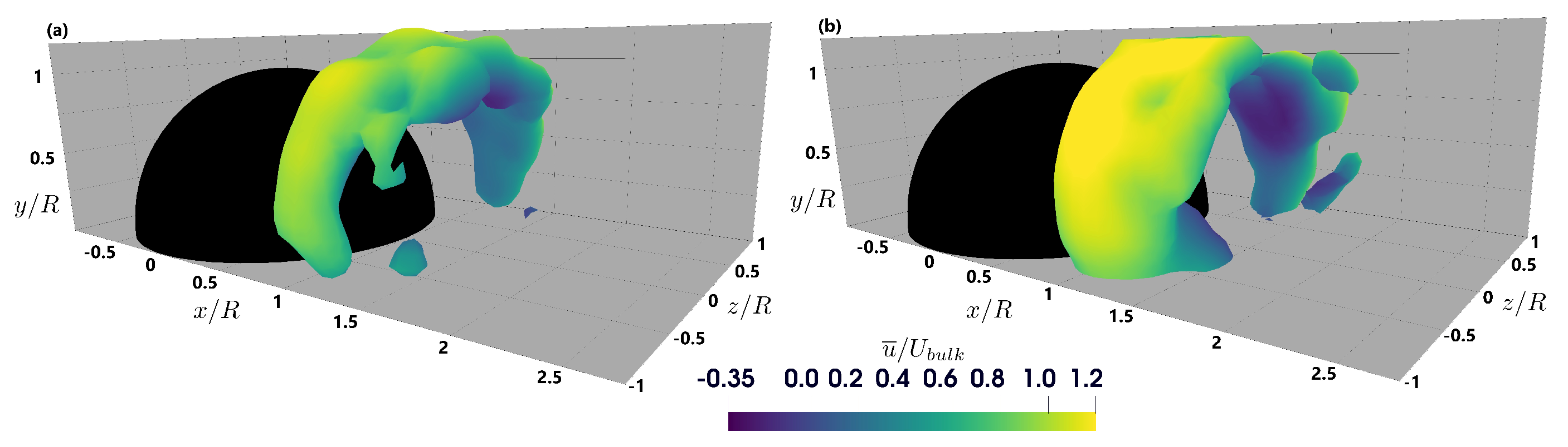
The isosurface of $\overline{u}/U_{bulk}$ = 0 in Figure 3 and Figure 4 represents the recirculation zone for each of the two RS. The submerged hemisphere produces a wake that exhibits complex three-dimensional separation, with variations in recirculation length and width depending on the RS. A lower RS produces a narrower wake, while a higher RS leads to a more extended and uniform recirculation region (Figure 3). For the single case at the lower submergence, the recirculation length decreased by approximately 16% at $y/R=0$ and by 6% at $y/R=0.5$ compared to the higher submergence. Furthermore, the spanwise width of the recirculation zone decreased by 17% at $y/R=0$, close to the hemisphere, for the lower RS (see

Table 2. Measured velocity parameters for the different cases.

Case	Recirculation Length at y/R = 0	Recirculation Length at y/R = 0.5	Maximum Wake Width at x/R = 1, y/R = 0	Wake Width at x/R = 4, y/R = 1
Single High	2.5R	2.61R	1.00R	0.61R
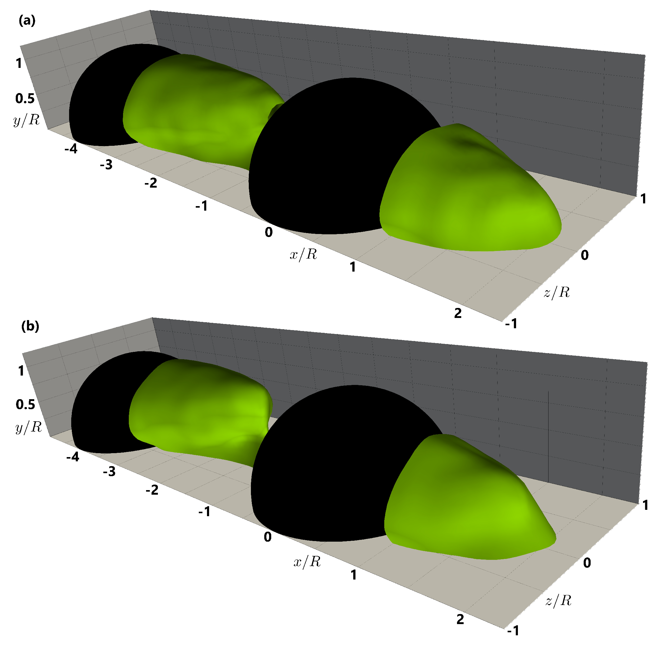
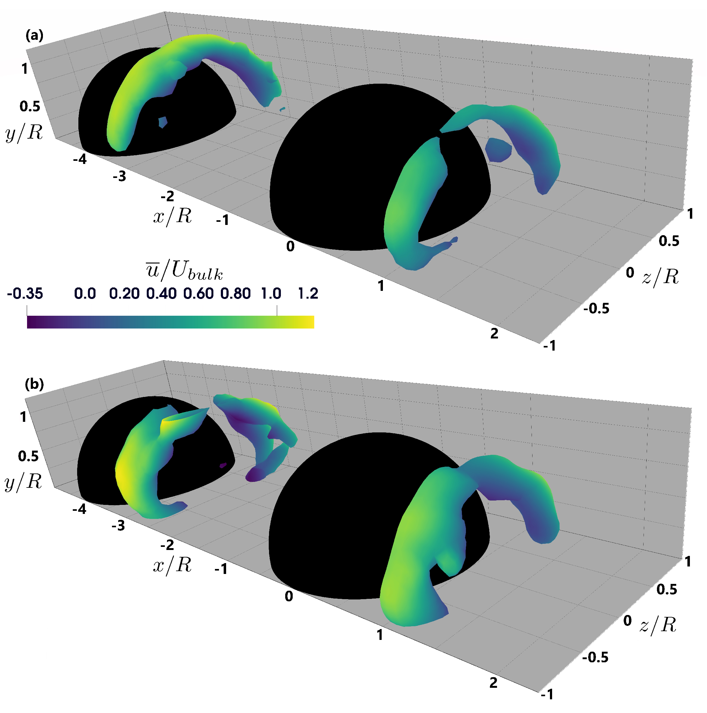
Single Low	2.15R	2.45R	0.83R	0.85R

). A small change in the shape of the recirculation zone behind the downstream hemisphere in the case with double hemispheres is visible in Figure 4. The recirculation zone extends the entire length between the hemispheres for the larger RS, creating an isolated reversed flow region. For the lower submergence, the recirculation between the hemispheres resembles the single hemisphere case but extends downstream with a narrow width and a height of y/R ≈ 0.15. A shorter and narrower recirculation zone results from a more rapid reattachment downstream of the single hemisphere at lower RS due to the obstacle’s increased relative influence on the flow. The higher RS results in a stable, isolated recirculation zone in the gap, since the greater flow depth reduces interactions between the hemispheres.

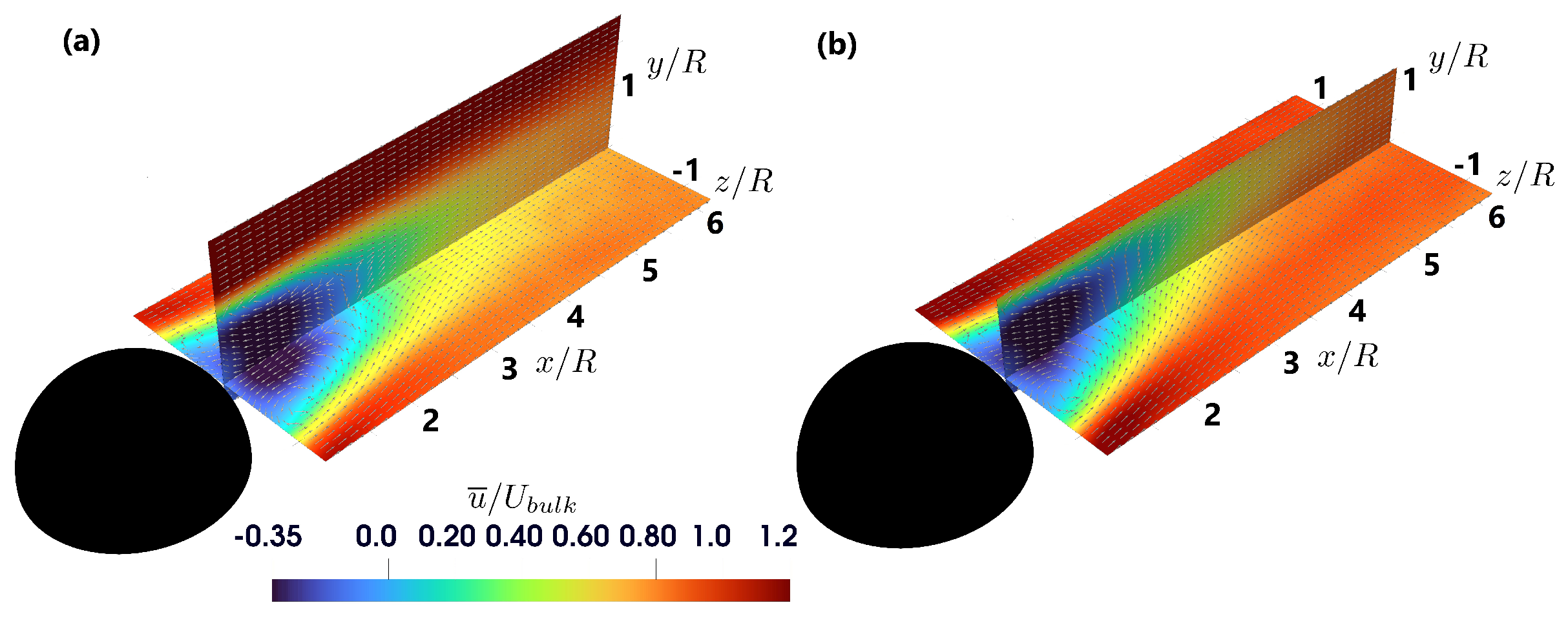
Figure 5 shows the development of time-averaged streamwise velocity, shown in the planes z/R = 0 and y/R = 0.25. At lower submergence, the wake remains narrower close to the hemisphere but broadens further downstream compared to higher submergence. In contrast, higher submergence results in a broader wake near the hemisphere, with the wake width remaining more uniform along the downstream distance. 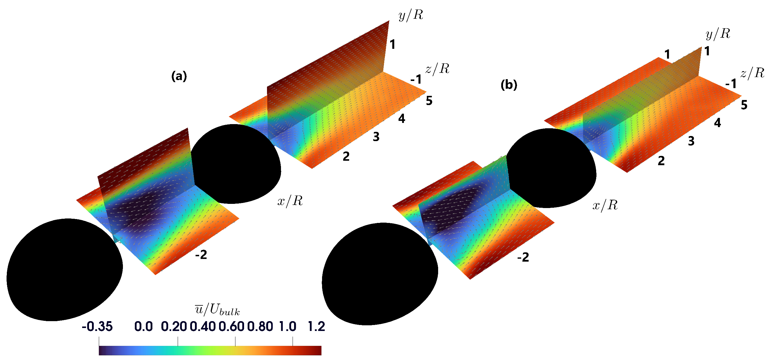The data in Table 2 show that the width of the zone with $\overline{u}/U_{bulk}<0.8$ is approximately 39% larger at x/R = 4 downstream of the hemisphere at a depth of y/R = 1 for the lower submergence. At lower RS, the obstacle’s higher relative prominence increases flow resistance, leading to larger low-velocity regions downstream. In the double hemisphere setup, lower RS leads to a narrower wake between the hemispheres, while higher RS creates a broader and more uniform velocity distribution between the obstacles. The streamwise velocity for the double hemisphere case shown in the planes z/R = 0 and y/R = 0.25 can be seen in Figure 6. Looking at the recirculation zone width shows that for the higher submergence, the area with $\overline{u}/U_{bulk}<0.8$ reaches a depth of y/R = 0.9. However, the lower submergence shows a width of 0.61R, similar to the width behind the single hemisphere at the higher submergence. Due to the reduced flow depth at lower RS, the wake exhibits stronger interactions and increased turbulence, which affects streamwise velocity recovery.

For all experimental cases, the horizontal centerline (z/R = 0) velocity profiles of the time-averaged streamwise velocity can be seen in Figure 7. Overall, a higher RS results in increased streamwise velocities. For the single hemisphere cases, Figure 7a,b, displays a higher velocity at y/R = 1 for the higher submergence throughout the entire length, with about 41% higher relative velocity at x/R = 3 compared to the lower submergence. Similar tendencies are shown in Figure 7c,d where the relative velocity at y/R = 1 is around 30% larger at x/R = 3 for the higher submergence. Between the hemispheres (Figure 7e,f), the velocity profiles show similar magnitudes, except for y/R = 1, which is approximately 56% higher for the larger submergence at x/R ≈ −1. The increased streamwise velocity at higher RS is due to reduced flow resistance from the more submerged obstacles. In contrast, at lower RS, the flow is more restricted by the bed and obstacles, resulting in lower velocities.

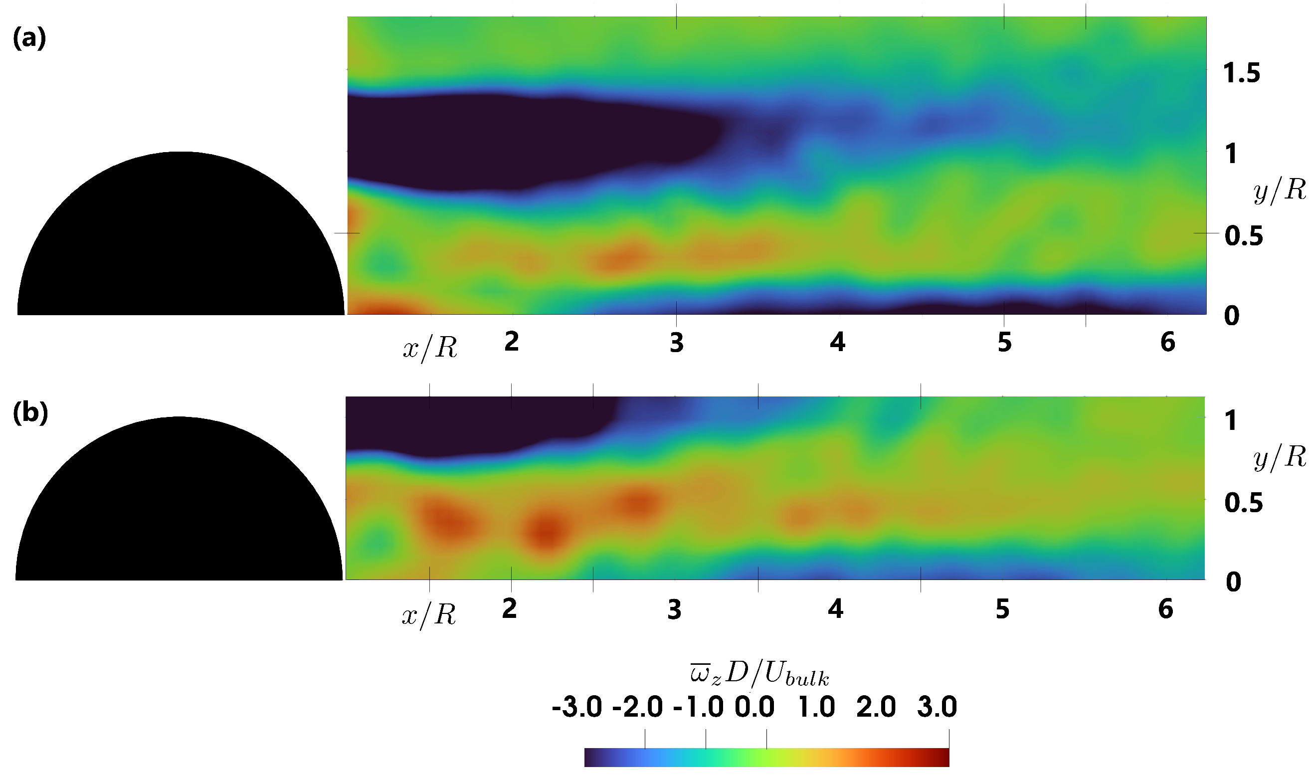
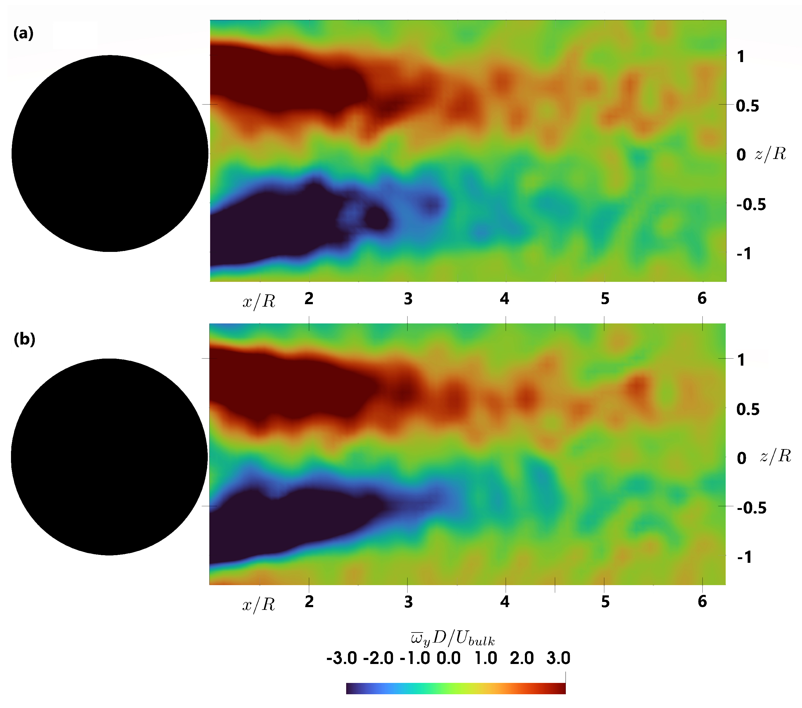
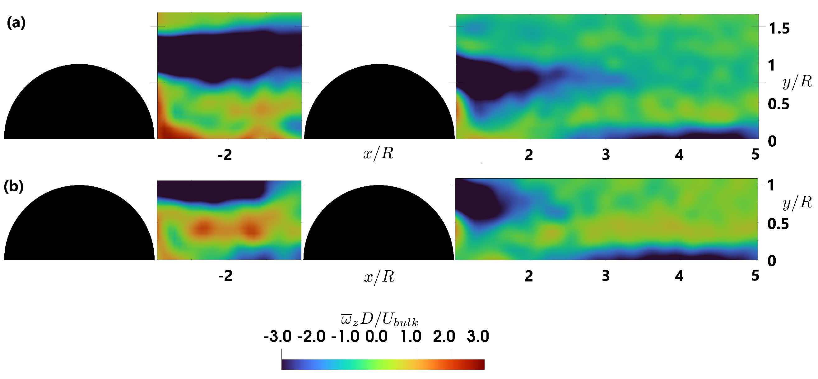
The time-averaged dimensionless transverse vorticity distribution is shown in Figure 8 and Figure 9. Planes located at y/R = 0.5 and z/R = 0 shows ${\overline{\omega }}_{y}D/U_{bulk}$ and ${\overline{\omega }}_{z}D/U_{bulk}$, respectively, for both submergences. The vorticity components are defined as ${\overline{\omega }}_y=\overline{{\displaystyle \frac{\partial u}{\partial z}}}-\overline{{\displaystyle \frac{\partial w}{\partial x}}}$ and ${\overline{\omega }}_z=\overline{{\displaystyle \frac{\partial v}{\partial x}}}-\overline{{\displaystyle \frac{\partial u}{\partial y}}}$. At lower RS, increased shear in the wake boundary layers enhances horizontal vorticity, expanding regions of negative vorticity in the horizontal plane. The peak value of the dimensionless horizontal vorticity component increased by about 23% for the lower submergence (see

Table 3. Summary of vorticity parameters. The first column presents the peak dimensionless transverse vorticity values. Subsequent columns indicate the length of regions with values less than −3 in horizontal and vertical planes.

Case	$\mid {\overline{\mathit{\omega }}}_{\mathit{y}}\mathit{D}/{\mathit{U}}_{\mathbf{bulk}}\mid$	${\overline{\mathit{\omega }}}_{\mathit{y}}\mathit{D}/{\mathit{U}}_{\mathbf{bulk}}<$−3	${\overline{\mathit{\omega }}}_{\mathit{z}}\mathit{D}/{\mathit{U}}_{\mathbf{bulk}}<$−3
Single High	7.51	2.32R	3.25R
Single Low	9.21	2.77R	2.64R
Double Low Behind	7.56	1.90R	1.57R

). In the horizontal plane, the area with negative vorticity below −3 increases 16% in length with decreased submergence. On the other hand, there is a 19% decrease in length in the vertical plane (Table 3).

Figure 10 and Figure 11 display the same quantities as in Figure 8 and Figure 9 but also include planes between the hemispheres. Similar to the single hemisphere case, the length of the area with negative vorticity below −3 increased by approximately $28\%$ in the horizontal plane, and by $40\%$ in the vertical plane for the lower submergence (see Table 3). Between the hemispheres, it is noticeable that the low vorticity area extends through the whole length of the vertical plane for the higher submergence. In the horizontal plane, the length increases with $24\%$ for the lower submergence, from x/R ≈ −1.7 to x/R ≈ −1.3. However, the proximity of the bed limits the formation of vertical vortices. At higher RS, reduced interaction with the bed allows vertical vortices to extend further. This results in a decrease in strength but an increase in spatial distribution.

To identify vortical structures, the Q-criterion, a widely used method for vortex detection in fluid flows, was applied [32]. Positive values of the Q-criterion identify regions where the rotation rate dominates over the strain rate, indicating the presence of turbulent vortex cores. It is defined as $Q={\displaystyle \frac{1}{2}}\left({\left|\right|\mathsf{\Omega }\left|\right|}^2-{\left|\right|S\left|\right|}^2\right)$, where $\left|\right|\mathsf{\Omega }\left|\right|$ represents the magnitude of the rotation rate tensor and $\left|\right|S\left|\right|$ denotes the magnitude of the strain rate tensor, herein normalized with ${(U_{bulk}/D)}^2$. Figure 12 and Figure 13 shows isosurfaces of $Q/{(U_{bulk}/D)}^2=3.5·{10}^{-6}$ which displays the arch vortex structure, colored by $\overline{u}/U_{bulk}$. The arch vortex extends further downstream for the lower RS for a single hemisphere, but a concavity region forms behind the boulder crest, shown in Figure 12. Regarding the case of double hemispheres, it is noticeable that the volume of the arch vortices decreases compared to the single case. The arch vortex splits behind the hemisphere crest for the lower submergence, conversely to the arch vortex behind the second hemisphere which was split at the higher submergence. The concave region behind the single hemisphere at lower RS is caused by stronger downward vertical velocity, enhancing dissipation in the wake. In contrast, the reduced volume of arch vortices at higher RS arises from less disturbed flows with a more defined vortex core.

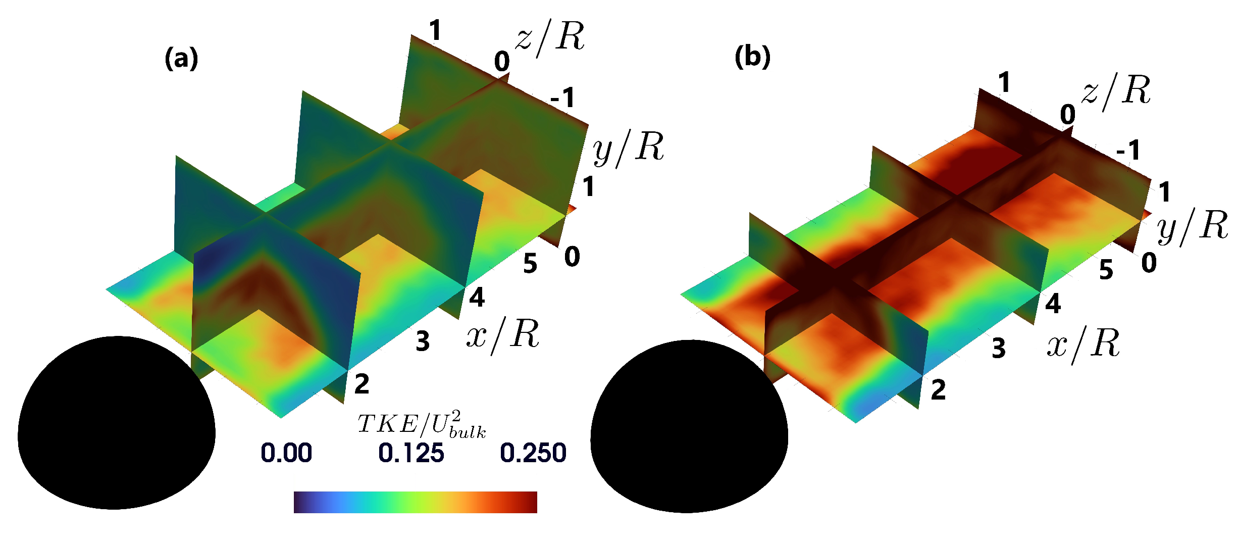
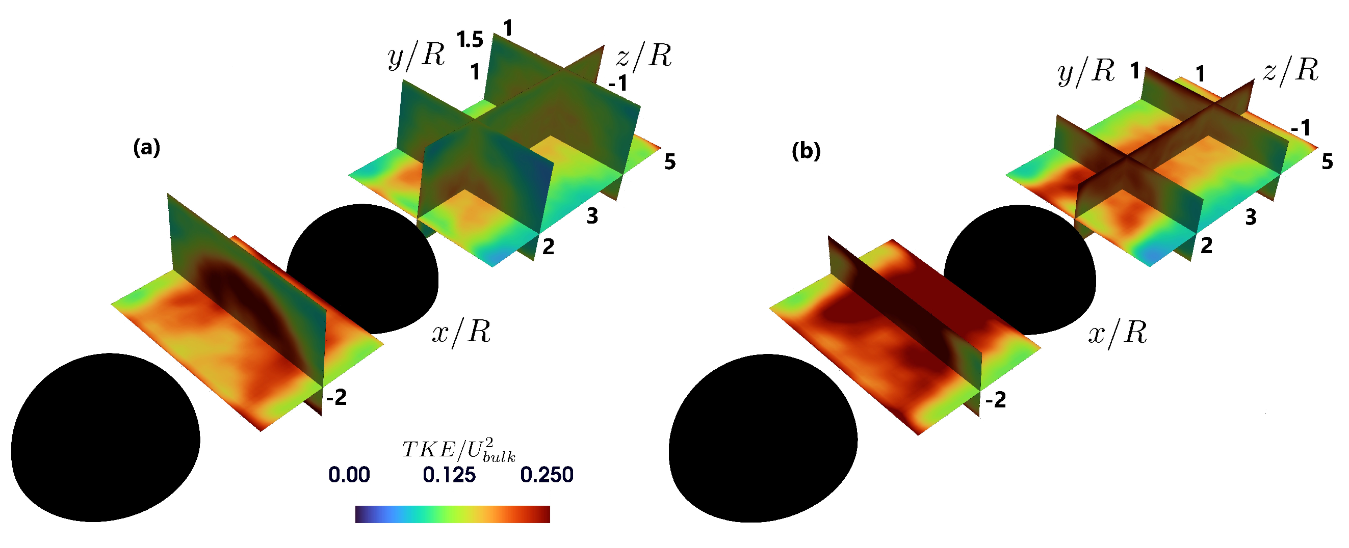
Figure 14 and Figure 15 show the change in time-averaged TKE/$U_{bulk}^2$ for the different submergences with the turbulent kinetic energy defined as TKE = 1/2($\overline{u^{\prime 2}}$ + $\overline{v^{\prime 2}}$ + $\overline{w^{\prime 2}}$) and planes at x/R = −2, 2, 4, 6, and y/R = 0.5. At lower RS, the interaction between the obstacle and the shallow flow increases turbulence, resulting in higher TKE values. A significant difference in TKE magnitude is observed for the single hemisphere case. For the higher submergence, a small area with TKE/$U_{bulk}^2$ > 0.2 appears directly downstream of the boulder at a height of y/R = 1. In contrast, for the lower submergence, an area with high TKE/$U_{bulk}^2\ge$ 0.25 extends from near the boulder and through the entire measurement volume. The distribution of TKE between the two hemispheres shows an increase in the area where TKE/$U_{bulk}^2\ge$ 0.25 for the lower submergence. For higher submergence, the TKE intensity is below 0.2 throughout the reconstruction volume behind the second hemisphere. However, for the lower submergence, the intensity reaches 0.3 in a small area near the second hemisphere. At higher RS, the wake becomes more dispersed, with energy distributed over a larger region, resulting in lower TKE values.

The periodicity of the near wake for the single hemisphere case was investigated by extracting the frequency of the oscillations at the point x/R = 2, y/R = 0.25, and z/R = 0. A Fourier transformation of the spanwise velocity component $w^{\prime }$ revealed the frequencies 0.45 and 1.55 Hz for the higher and lower submergences, respectively. The corresponding Strouhal numbers, $St=fD/U_{Bulk}$, was St = 0.19 and St = 0.49, respectively.

4. Discussion

This study investigated how the change in RS affected wake structure and the flow field adjacent to large boulder-like obstacles, here idealized as hemispheres. These obstacles can have many important properties in a regulated river, such as providing favorable habitats and resting places for fish and benthic fauna. Conducting extensive hydraulic research can serve as a valuable resource in designing habitat structures more efficiently. Compared to previous numerical and experimental studies of turbulent flow around 3D bluff bodies (spheres, hemispheres, and boulders), the data reported in this work show consistency with established trends while providing additional insights into the influence of relative submergence.

The narrow width of the flume likely introduced some unintended effects on the flow field due to the close proximity of the sidewalls to the hemispheres. These effects are likely minor and have a small influence on the wake structures and recirculation zones. Despite this limitation, the observed trends, such as the influence of relative submergence on turbulence and velocity distribution are consistent with previous research. Additionally, employing time-resolved 3D-PTV provides an improved understanding of these dynamics. Future work could explore this by performing experiments in wider flumes to reduce sidewall effects and confirm the trends identified in this study.

The results of this investigation demonstrate that velocity, vorticity, TKE, and general flow patterns change with varying submergence. The change in the wake’s shape can be partially attributed to an increased downward vertical velocity from the hemisphere crest, as demonstrated by Nilsson et al. [33]. The main effect of adding the second hemisphere was a decrease in the recirculation length, velocity magnitude, the volume of the arch vortices, and the vorticity and TKE regions behind the downstream hemisphere. For the single hemisphere case, decreasing the submergence from 2 to 1.5 resulted in a 16% reduction in the recirculation length at bed level. A similar relationship between submergence and recirculation zone was observed by Golpira et al. [15]; they demonstrated a drop of 23% when lowering the submergence for a natural boulder from 2 to 1.3. Additionally, for the double hemisphere case, the recirculation length increased and spanned the whole length between the hemispheres, the wake behind the upstream hemisphere is affected by the downstream hemisphere and disturbs the recovery of the streamwise velocity. Barman et al. [10] also demonstrated reduced streamwise velocity between two inline hemispheres with similar spacing. The velocity profiles reveal higher velocities close downstream of the single boulder and between the boulders in the double-hemisphere case at y/R = 1 for the higher submergence. This indicates that influences from the free surface may affect the velocity magnitude at lower submergence levels. Close to regions with larger TKE magnitudes, the arch vortex tends to extend further streamwise. The periodic oscillations of the near wake were investigated for the single hemisphere case, through the dimensionless Strouhal number, and revealed a dimensionless frequency of the vortex shedding between 0.19 and 0.49. These findings are consistent with Tu et al. [9], who reported a Strouhal number of $St=0.47$ in the near wake of a hemisphere, and with a numerical study by Cao et al. [34], which found $St=0.17$.

This study highlights several parameters that the IPOS framework [18] identifies as important for fish swimming in altered flows: flow Intensity (vorticity and TKE), Periodicity (frequency, e.g., Strouhal number), Orientation (recirculation and direction of dominant fluctuations), and Scale (Reynolds number). Measuring these parameters can be beneficial when conducting experiments with fish to couple hydraulic parameters with behavior. Currently, there is a lack of volumetric time-resolved measurement data combined with fish studies, which could offer deeper insights into fish behavior than time-resolved pointwise measurements, as illustrated in Smith et al. [17]. Incorporating volumetric measurements would provide a more comprehensive understanding of how fish interact with complex flow environments. This type of experimental result can also be used when designing versatile habitats and natural fishways that enable a diversity of species. Based on the presented results, it is possible to qualitatively discuss some potential effects on fish habitats due to the variations in submergence and the addition of a second roughness element. Firstly, the recirculation zone behind the single hemisphere was reduced for the lower submergence; this may diminish the possibility for energy conservation close to the hemisphere compared to the higher submergence. A wider area with lower velocity occurs, which may enable fish with weaker swimming capacity to reduce energy expenditure. Secondly, in the double hemisphere case, the higher submergence provides an isolated reversal flow area between the hemispheres, which can be utilized for resting. Additionally, the decrease in the length of the recirculation zone and vorticity areas occurring behind the downstream hemisphere results in smaller eddies and may be preferred by fish to maintain stability and lower muscle activity. Thirdly, in both experimental cases, higher turbulence levels were observed for the lower submergence, which could make this scenario unfavorable for the fish when attempting to minimize energy expenditure. However, it may also imply that fish with larger body lengths are capable of swimming at higher speeds in this scenario. Measurements with lower RS would have been of great interest but here, we were limited by the height of the reconstruction volume due to the limitations of the measurement system and the flume. The narrow width of the flume in combination with optical access only through the side wall limited the smallest flow depth possible to capture by the four-camera system as the free water surface was disturbing the measurements and needed to be cropped out of the frames.

5. Conclusions

This study provides measurements of the flow field around single and double in-line mounted hemispheres for two relative submergences, utilizing time-resolved 3D PTV. In contrast to earlier studies that used planar or pointwise measurements, this research employs 3D-PTV to analyze three-dimensional flow dynamics around a hemisphere under different submergence conditions. By capturing detailed wake structures and turbulence characteristics, the findings provide valuable data to support hydraulic model calibration and guide habitat design in shallow waterways, focusing on recirculation, turbulence, and energy conservation zones.

The results indicate that relative submergence impacts the wake characteristics and flow field dynamics. For individual hemispheres, lower submergence levels led to a 16% reduction in the recirculation length at the bed level and a 17% reduction in spanwise width near the obstacle. Additionally, larger low-velocity regions were observed downstream, which may benefit fish by providing zones of reduced energy expenditure. The addition of a second hemisphere increased the flow field’s complexity by introducing interference effects, such as isolated wake regions at higher submergences.

This study demonstrates the effectiveness of time-resolved 3D particle tracking velocimetry in measuring and quantifying key parameters related to fish swimming and habitat, exemplified through the IPOS framework. A qualitative discussion of results obtained from measurements concerning fish habitats suggests that higher submergence may be preferred by fish, in terms of greater possibilities for energy conservation. The findings of this study can be used to verify and improve numerical modeling of free surface flows around roughness elements with low relative submergences.

Future work that utilizes larger and more nature-like roughness elements in combination with lower relative submergences, conducted in wider flumes, may provide valuable insights into how the flow field in a natural stream might be affected by changes in flow depth. Experiments involving fish and time-resolved turbulent flow parameters would also provide valuable insights for the ecohydraulic community.