Stack Coupling Machine Learning Model Could Enhance the Accuracy in Short-Term Water Quality Prediction

Abstract

Traditional river quality models struggle to accurately predict river water quality in watersheds dominated by non-point source pollution due to computational complexity and uncertain inputs. This study addresses this by developing a novel coupling model integrating a gradient boosting algorithm (Light GBM) and a long short-term memory network (LSTM). The method leverages Light GBM for spatial data characteristics and LSTM for temporal sequence dependencies. Model outputs are reciprocally recalculated as inputs and coupled via linear regression, specifically tackling the lag effects of rainfall runoff and upstream pollutant transport. Applied to predict the concentrations of chemical oxygen demand digested by potassium permanganate index (COD) in South China’s Jiuzhoujiang River basin (characterized by rainfall-driven non-point pollution from agriculture/livestock), the coupled model outperformed individual models, increasing prediction accuracy by 8–12% and stability by 15–40% than conventional models, which means it is a more accurate and broadly applicable method for water quality prediction. Analysis confirmed basin rainfall and upstream water quality as the primary drivers of 5-day water quality variation at the SHJ station, influenced by antecedent conditions within 10–15 days. This highly accurate and stable stack coupling method provides valuable scientific support for regional water management.

1. Introduction

As one of the most critical sources of water for irrigation purposes, industrial needs, residential water consumption and other uses worldwide, surface water can have a significant impact on the sustainable use of water resources and on human health and future development strategies [1,2,3]. According to a study that calculates the collective threat index using digital river networks and ocean systems, 80% of the world’s population lives in areas where water security threats may exceed 75% [4]. Therefore, it is very important to maintain the good quality of surface water in rivers for sustainable development and safety to human health [5,6,7]. The dynamic nature of the river systems and their easy accessibility for waste disposal make the river systems most vulnerable to the adverse effects of environmental pollution. Evaluation and prediction of the surface water quality is necessary for effective management of river basins so that sufficient measures can be adopted to ensure that the pollution levels remain within permissible limits [8]. Especially in recent years, the continual expansion of real-time water quality monitoring networks is driving a growing demand for rapid and high-accuracy prediction systems to support comprehensive water environmental management and protection by regulatory agencies worldwide. As the basis of water pollution control, a water quality model is usually used to predict the trend of water quality based on the current situation of water quality, meteorological conditions and pollution discharge level [9].

Water quality can be divided into biological water quality, water form water quality, and physical and chemical water quality by different evaluation indexes [10]. Of these, physical and chemical water quality variables are widely used in surface water quality modeling [11]. Many studies have attempted to estimate the river water quality using conventional process-based modeling methods, such as IWA River Quality Model No. 1 [12], QUAL2K [13], WASP6 [14], which have offered comparatively accurate predictions for water quality parameters. In addition, there have been some attempts to simulate water quality based on statistics, assuming that there is a correlation between prediction variables and response variables, which is essentially normal distribution and linear distribution. However, due to the impacts of human activities such as urbanization, industrialization, agricultural irrigation, and water-related engineering projects, as well as the complex external environmental constraints of river basins such as seasonal fluctuations in precipitation and extreme weather events, water system processes in the real world are diverse and complex. Traditional data processing technology cannot effectively address the uncertainty of the mechanisms and variables upon which simulation depends or the deviation of field data collection [15,16]. In recent decades, AI (Artificial Intelligence) models, which have been considered as an effective alternative method for modeling complex nonlinear systems, become an another prediction and classification tool that can overcome the limitations of the traditional process-based models and statistical models [17]. In those models, the correlation between input and output is the key factor in the construction of the model, while the internal complex processes of the water system are no longer considered. Many recent studies of water quality modeling have mentioned AI models, which could be divided into artificial neural network (ANN) model, Adaptive Neuro-Fuzzy Inference System (ANFIS)-based model, kernel-based models like support vector machine (SVM), tree-based models like decision tree (DT), complementary model, hybrid model combined with more than one models or techniques and other meta-heuristic models that come from different model classifications [18], could obtain more accurate results in the prediction of nonlinear water quality processes [19,20]. For instance, Huang and Foo [21] predicted the salinity change in river water due to salinity intrusion which may affect aquatic life, for which the ANN model could correlate various variables, such as flow, rainfall and fresh water flow, with high accuracy and cost effectiveness. Heddam [22] studied the efficiency of Radial Basis Neural Network (RBNN) and Multilayer Perceptron (MLP) algorithms in modeling DO contents in Klamath and Link River, USA, using four water quality variables. Gebler et al. [23] fit the response relationship between ecological indicators, water pollution, and hydrological form degradation in using various biological indicators and physical and chemical parameters with ANN. Yan et al. [24] classified the water quality of all the major rivers of China using ANFIS. The result showed that the ANFIS-based model could lead to better efficiency for river water quality, and the performance was better than that of ANN models. Ahmed and Syed Mustakim Ali [25] examined the performance of ANFIS in biochemical oxygen demand (BOD) prediction, and obtained satisfactory results. Furthermore, Kamyab-Talesh et al. [26] used SVM to identify the contribution of water quality parameters affecting water quality index (WQI). The results showed that nitrate had the greatest influence on WQI, and the model could achieve high satisfaction. Ho et al. [27] used the decision trees of different input scenarios, which simplify the complex data and reduce nonlinearity caused by water quality predictions, to predict the water quality index and the results have certain reference significance. As a pre-processing tool for managing high-dimensional data, Maier and Keller [28] used principal component analysis (PCA) combined with k-nearest neighbors (k-NN), Random Forest (RF), SVM, RF, support vector machine, multivariate adaptive regression spline (MARS), and extreme gradient boost (XGB) models, respectively. Compared with the original model, the coupled regression model based on PCA had higher accuracy, less error, and the ability to deal with high-dimensional regression problems.

The consensus is that with the development of machine learning algorithm, the accuracy of water quality prediction was improving; however, considering that the variations in river water quality were affected by the lag stack of previous time-series data, and were limited by its spatial dependence on the environmental characteristics of the river basin on the other hand, there is no particular model that can surpass other models in terms of performance. Therefore, using integration technology to couple different models may lead to more accurate results in solving spatio-temporal dependence and would be worthy of further research. There have been several studies suggesting coupled algorithm models to address the extreme complexity of real-world sequence dataset modeling, for example, to solve the “noise signals” which often appear in water quality data and could probably make prediction more difficult. Najah et al. [29] compared a normal ANFIS-based model and wavelet de-noising techniques with ANFIS, and the coupled model proved to be superior and faster than ANFIS. Jin et al. [30] coupled a genetic algorithm (GA) and ANN model to make up for the inherent defects of an artificial neural network model; by the sliding window prediction pattern, the coupled model investigated the variation in variables and optimized the initial weight to prevent a local optimal solution, which improved the final prediction. Faruk [31] used ANN, ARIMA and coupled ANN-ARIMA model to predict water quality variables, which showed that the coupled model, by using ANN and ARIMA to deal with the nonlinear and linear response data, respectively, is more reliable than ANN and ARIMA model.

In the current literature review, most studies focus on water quality simulation based on machine learning to compare the performance, efficiency, and applicability of different AI algorithms. Some of them utilize coupling algorithms to address the limitations of data-driven models. However, most of these approaches target single-domain constraints and lack a multi-faceted strategy for algorithmic innovation—such as the integrated extraction of spatiotemporal latent features [32]. Therefore, our current work focuses on the stack coupling of two machine learning methods, and introduces a nested forecasting methodology for water quality that leverages a stacked ensemble of heterogeneous models. The framework employs hierarchical spatiotemporal feature extraction followed by meta-learning-based decision fusion to improve predictive accuracy. Specifically, Light GBM, an improved gradient boosting machine, and a special recurrent neural network algorithm, known as long short-term memory (LSTM) are used. And the aim is to improve prediction accuracy and model interpretability. In this approach, the Light GBM model is built to capture association patterns between different source types and spatial attribute data, while the LSTM model is constructed to identify the implicit stacking lag effect in time-series data. Since then, the simulation results of the two models are recalculated as input variables for one another and then integrated to a meta-learner based on linear regression, yielding the final prediction. This coupling model effectively addresses the challenge of fitting the time lag stacking effect with complex spatial data characteristics in regional water quality prediction and compensates for the inability to capture patterns of different spatial data characteristics in water quality time-series prediction. The method was subsequently validated in the Jiuzhoujiang river basin to predict the 5-day-later concentrations of chemical oxygen demand digested by potassium permanganate (COD). The primary objectives of this study are as follows:

• To verify the correctness of the gradient boosting method in predicting water quality parameters using the Light GBM algorithm and to analyze the contribution of different sources of data to water quality changes.
• To confirm the effectiveness of LSTM algorithm in the estimation of the parameters of water quality and to identify the stacking lag response period of time-series data in water quality parameters prediction.
• To develop and validate a new method of coupling models to predict the water quality parameters in the Jiuzhoujiang river basin based on the experimental data for the period of 2019–2021.
• Furthermore, to mitigate reduced feature interpretability caused by multicollinearity, we employed the variance inflation factor (VIF) for feature selection prior to model construction and comparison.

2. Methodology

Figure 1 shows a schematic description of the methodology used in this study which can be divided into three parts: model pre-processing; baseline model simulation; and coupling model prediction. Together with the model performance metrics, those parts will be described in detail in the following sections. Stack coupling refers to the output of baseline simulation as new input features for both models (as in red square).

2.1. Model Pre-Processing and Performance Metrics

2.1.1. Data Pre-Processing

Data normalization is one of the important pre-processing steps in the development of machine learning models. It is more efficient for most machine learning models to train with the normalized data. Particularly in ANN or SVM models, appropriate data normalization is critical for enhancing computational efficiency and reducing sensitivity to variations in input data feature scales [33]. There are many normalization techniques such as min-max, z-score, and median, etc. In a comparative analysis utilizing the ANN model, Antanasijević et al. [34] evaluated multiple normalization methods and identified min-max normalization as a straightforward yet effective technique. Min-max normalization performs a linear transformation on the original data, enabling features with different units and scales to be computed and compared on a unified scale, without altering the underlying distribution of the data [35]. Previous studies have employed approaches ranging from simple [0, 1] scaling to range-specific normalization, with the choice largely dependent on whether such transformations unduly affect modeling accuracy [36,37]. In this study, with outliers removed prior to acquisition and the remaining deviations within an acceptable range, the min-max normalization (Equation (1)) was adopted, which converts the input into a more available form:

$$D^{\prime }={\displaystyle \frac{D-D_{min}}{D_{max}-D_{min}}}$$

(1)

where D is the original data, and D′ is the normalized data.

Due to sensor failures, network failures or other accidents, automatic water quality monitoring stations may have problems such as missing data and exception data in the course of operation. These abnormal phenomena will eventually lead to excessive deviation between the predicted results and the actual monitoring values of water quality. Because time is irreversible, the missing data or exception data cannot be obtained again, so those data should be estimated as accurately as possible to improve the prediction accuracy. In current studies, the common processing method is to fill or replace those parts of the data, and then predict the water quality. As long as the method is proper, the result is satisfactory.

2.1.2. Input Selection

Since there are extensive problems of multicollinearity and correlation, it is necessary to obtain a set of input datasets that are mutually independent but significantly related to the model output. This process is typically achieved through feature selection [38]. As a critical step in handling high-dimensional data in regression and classification, feature selection serves to reduce computational complexity, mitigate the curse of dimensionality [39], shorten training time, and improve predictor performance [40]. Dependency metrics, such as correlation analysis, could be a good choice. Thus, the correlation coefficient threshold screening and variance inflation factor (VIF) analyses were applied in this study.

The correlation coefficient threshold screening method calculates the correlation coefficient matrix of the input feature dataset and determines the upper limit value, which is used to eliminate the input features whose correlation coefficient value is higher than the threshold. Since the original data did not conform to a normal distribution according to the Kolmogorov–Smirnov test, we employed Spearman’s rank correlation coefficient (Equation (2)) for subsequent analysis [41]. When all ranks are distinct integers, it can be calculated as Equation (3).

$$\rho ={\displaystyle \frac{\frac{1}{n}{{\displaystyle \sum }}_{i=1}^n\left(R(x_i)-\overline{R\left(x\right)}\right)\left(R(y_i)-\overline{R\left(y\right)}\right)}{\sqrt{\frac{1}{n}{{\displaystyle \sum }}_{i=1}^n{\left(R(x_i)-\overline{R\left(x\right)}\right)}^2{\left(R(y_i)-\overline{R\left(y\right)}\right)}^2}}}$$

(2)

$$\rho =1-{\displaystyle \frac{6{{\displaystyle \sum }}_{i=1}^n{d}_i^2}{n\left(n^2-1\right)}}$$

(3)

where R(x) and R(y) denote the ranks of x and y, respectively, $\overline{R\left(x\right)}$ and $\overline{R\left(y\right)}$ represent their mean ranks, and d_i is the difference between the two ranks of each observation. To aid the validation of input parameter selection via the VIF method, we employed a more lenient threshold of 0.85 [42,43].

VIF quantifies the degree of linear dependence between each independent variable and all others in a regression model [44]. It indicates the extent to which the variance of a regression coefficient is inflated due to multicollinearity, and could be calculated as Equation (4), where R² is the determination coefficient of the regression model.

$$VIF={\displaystyle \frac{1}{1-R^2}}$$

(4)

Generally speaking, if no collinearity exists among the input variables, all VIF values would be 1, while a value above 1 suggests some correlation with other variables. Values between 5 and 10 denote a high correlation that could undermine regression accuracy, while any value exceeding 10 confirms severe multicollinearity that critically distorts model estimates, widens confidence intervals, and compromises the reliability of significance tests [45,46]. In many studies, the variable with VIF value > 10 would be removed from the model [47], while a more stringent VIF threshold of 5 is often adopted when tighter constraints on model inputs are required to enhance reliability or extract specific information [48].

2.1.3. Performance Metrics

Many statistical indicators could be used to evaluate the performance and efficiency of the model, such as determination coefficient or adjusted determination coefficient (R² or Adj. R²), Mean Absolute Error (MAE), Nash–Sutcliffe efficiency coefficient (NSE), Mean Absolute Percentage Error (MAPE), Root Mean Square Error (RMSE), correlation coefficient (CC) and Standard Error of Prediction (SEP). In order to measure the efficiency and performance of the model from multiple aspects, the evaluation index should include at least one goodness-of-fit and at least one absolute error measure [49]. Considering the similarity of the index structure and the feasibility of comparing different input dataset models in this paper, Adj. R² (Equation (5)), NSE (Equation (7)), RMSE (Equation (8)) and MAPE (Equation (9)) were selected to measure the prediction performance of the proposed models in this study as follows:

$$Adj. R^2=1-{\displaystyle \frac{\left(1-R^2\right)\left(n-1\right)}{\left(n-k-1\right)}}$$

(5)

where k was the number of input variables. R² was calculated as follows:

$$R^2={\left({\displaystyle \frac{{{\displaystyle \sum }}_{i=1}^n\left(y-\overline{y}\right)\left(y^{\prime }-\overline{y^{\prime }}\right)}{\sqrt{{{\displaystyle \sum }}_{i=1}^n{\left(y-\overline{y}\right)}^2{{\displaystyle \sum }}_{i=1}^n{\left(y^{\prime }-\overline{y^{\prime }}\right)}^2}}}\right)}^2$$

(6)

$$NSE=1-{\displaystyle \frac{{{\displaystyle \sum }}_{i=1}^n{\left(y-y^{\prime }\right)}^2}{{{\displaystyle \sum }}_{i=1}^n{\left(y-\overline{y}\right)}^2}}$$

(7)

$$RMSE=\sqrt{{\displaystyle \frac{1}{N}}{\displaystyle \sum }_{i=1}^n{\left(y^{\prime }-y\right)}^2}$$

(8)

$$MAPE={\displaystyle \frac{1}{N}}{\displaystyle \sum }_{i=1}^n\left|{\displaystyle \frac{y-y^{\prime }}{y}}\right|\times 100\%$$

(9)

where $y$, $y^{\prime }$, $\overline{y}$ and $\overline{y^{\prime }}$ are the observed value, predicted value, average of the observed values, and average of the predicted values, respectively.

2.2. Light GBM

Gradient boosting algorithm is a new supervised ensemble learning technique for regression and classification problems, which produces prediction models in the form of sets of weak prediction models [50]. It develops models in a stage-wise fashion as in other boosting methods, but improves the accuracy by allowing optimization of an arbitrary differentiable loss function [51]. Based on its efficiency, accuracy, interpretability and robustness, the algorithm has become a widely used machine learning algorithm [52,53]. When typical decision trees are used as weak prediction models, the algorithm can be called a gradient boosting decision tree (GBDT). There are several different branches according to the strategy of decision tree growth, such as level-wise tree growth and leaf-wise tree growth [54]. In 2017, as a distributed and highly efficient GBDT improved model, LightGBM was released by Microsoft research Asia distributed Machine learning toolkit (DMTK) team [55] to solve the accuracy and efficiency reduction caused by large amounts of data and high-dimensional processing [56,57]. Compared with other GBDT-based algorithms such as AdaBoost, XGBoost or CatBoost [58,59,60], LightGBM provides three algorithms to elevate its performance, which can be called Histogram-based algorithm, Gradient-based One-Side Sampling (GOSS) and Exclusive Feature Bundling (EFB). Under the Histogram-based algorithm, continuous features can be discretized into so-called k bins with the same index in each bin [55]. Thus, split points of decision trees can be determined by only k bins. As a weak study model in the algorithm, the overall accuracy should not be reduced whether split points were best or not. On the contrary, the segmentation based on bins could have a certain effect of inhibiting over-fitting [57]. GOSS is a sampling method based on the gradient of data instance, which can keep all the large gradient instances and randomly sample the small gradient instances. That is, after sorting all data instances by gradient, the top a% of the data instances are selected firstly, and then b% of the remaining data instances are randomly selected. Thus, more attention is paid to the undertrained data instances without changing the data distribution to ensure the learning accuracy of the decision tree. EFB is a method to reduce the size of training parameters by using the sparsity of high-dimensional data. In other words, the mutually exclusive features are bound to different features with lower density in high-dimensional data, which can effectively avoid unnecessary calculation of zero eigenvalues. Specific algorithms are shown below (Algorithms 1–4), and further details can be found in the paper [55].

Algorithm 1: Histogram-based Algorithm

1: Input: I: training data, d: max depth

2: Input: m: feature dimension

3: note Set ← {0} ▷ tree nodes in current level

4: row Set ← {{0, 1, 2, …}} ▷ data indices in tree nodes

5: for i = 1 to d do

6:  for node in node Set do

7:   usedRows ← row Set[node]

8:   for k = 1 to m do

9:     H ← new Histogram ()

10:    ▷ Build histogram

11:    for j in usedRows do

12:     bin ← I.f[k][j].bin

13:     H[bin].y ← H[bin].y + I.y[j]

14:     H[bin].n ← H[bin].n + 1

15:    Find the best split on histogram H.

16:    ...

17:  Update rowSet and nodeSet according to the best split points.

18:  ...

Algorithm 2: Gradient-based One-Side Sampling

1: Input: I: training data, d: iterations

2: Input: a: sampling ratio of large gradient data

3: Input: b: sampling ratio of small gradient data

4: Input: loss: loss function, L: weak learner models ← {}, fact ← (1 − a)/b

5: topN ← a × len(I), randN ← b × len(I)

6: usedRows ← row Set[node]

7: for i = 1 to d do

8:   preds ← models.predict(I)

9:   g ← loss(I, preds), w ← {1, 1, ...}

10:  sorted ← GetSortedIndices(abs(g))

11:  topSet ← sorted[1: topN]

12:  randSet ← RandomPick(sorted[topN: len(I)], randN)

13:  usedSet ← topSet + randSet

14:  w[randSet] × = fact. Assign weight fact to the small gradient data.

15:  newModel ← L(I[usedSet], − g[usedSet], w[usedSet])

16:  models.append(newModel)

Algorithm 3: Greedy Bundling

1: Input: F: features, K: max conflict count

2: Construct graph G

3: searchOrder ← G.sortByDegree()

4: bundles ← {}, bundlesConflict ← {}

5: for i in searchOrder do

6:   needNew ← True

7:   for j = 1 to len(bundles) do

8:    cnt ← ConflictCnt(bundles[j],F[i])

9:    if cnt + bundlesConflict[i] ≤ K then

10:    bundles[j].add(F[i]), needNew ← False

11:    break

12:  if needNew then

13:   Add F[i] as a new bundle to bundles

14: Output: bundles

Algorithm 4: Merge Exclusive Features

1: Input: numData: number of data

2: Input: F: One bundle of exclusive features

3: binRanges ← {0}, totalBin ← 0

4: usedRows ← row Set[node]

5: for f in F do

6:   totalBin += f.numBin

7:   binRanges.append(totalBin)v

8: newBin ← new Bin(numData)

9: for i = 1 to numData do

10:  newBin[i] ← 0

11:  for j = 1 to len(F) do

12:   if F[j].bin[i] = 0 then

13:    newBin[i] ← F[j].bin[i] + binRanges[j]

14: Output: newBin, binRanges

2.3. Long Short-Term Memory

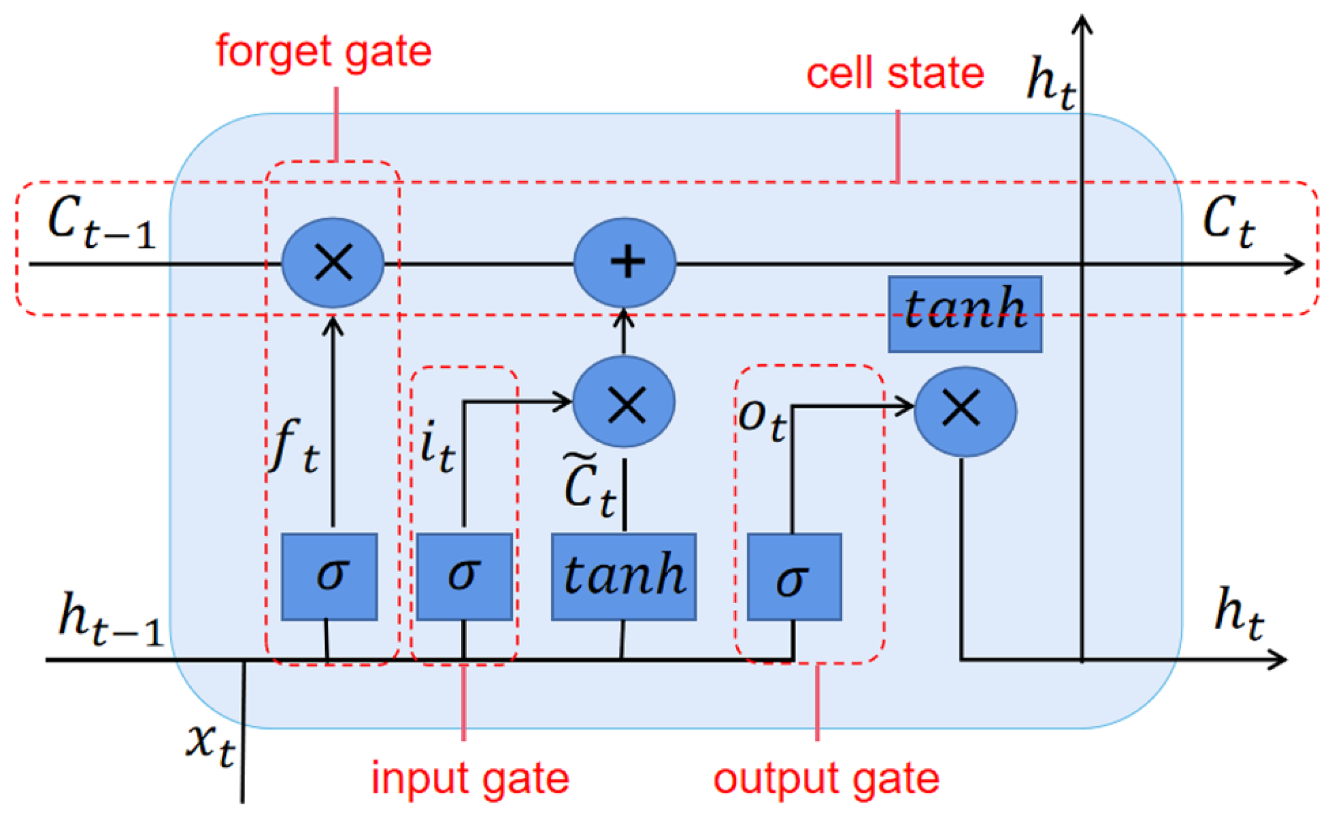
An artificial neural network (ANN) is a machine learning algorithm based on the structure of biological neural network, which can simulate complex nonlinear relationships even if the explicit form of the relationship between variables is unknown [61,62]. The basic artificial neural network structure consists of an input layer, a series of hidden layers and an output layer, each of which is composed of many nonlinear algebraic function node elements called interconnected neurons [63,64]. Since a traditional neural network cannot capture the sequence information features in the input dataset, it is difficult to use the previous information to fit the follow-up events [65]. To solve the problems above, a recurrent neural network (RNN), with the ability of memory, is widely considered useful. By increasing the horizontal connections between hidden layer elements and using the weight matrix to transmit the values of neural nodes between different time series, RNN is able to perform cyclic continuous operation on sequence information [66]. However, when dealing with long-term dependence, the calculation of the connection between nodes that are far away in the time series will involve multiple multiplication of Jacobian matrix, which will lead to gradient explosion or gradient vanishing [67]. To solve this problems, an LSTM neural network, which is faster and easier to converge to the optimal solution than other traditional neural networks when dealing with time sequence prediction problems, was proposed [68]. The structure of an LSTM network is shown in Figure 2 [68], in which x means the input; h and C reference hidden state vector and cell activation vector; o is the logistic Sigmoid function; and tanh is to ensure the values are between −1 and 1.

• Forget gate layer: Whether the previous cell state would be forgotten in the current cell is determined in this layer. The current input x_t and the previous hidden state h_t−1 are passed through and the output of the layer is calculated by Equation (10). A value of f_t of 0 or 1 refers to the state of being forgotten or retention.

$$f_t=\delta \left(w_f·\left[h_{t-1}, x_t\right]+b_f\right)$$

(10)

• Input gate layer: There are two memory vectors to decide the output value in this layer, which can be called as sigmoid vector and tanh vector, and can be calculated by Equation (11) and Equation (12), respectively.

$$i_t=\delta \left(w_i·\left[h_{t-1}, x_t\right]+b_i\right)$$

(11)

$$\widetilde{C_t}=tanh\left(w_f·\left[h_{t-1}, x_t\right]+b_f\right)$$

(12)

Finally, the value of the cell state is updated as follows (Equation (13)).

$$C_t=f_t\times C_{t-1}+i_t\times \widetilde{C_t}$$

(13)

• Output gate layer: The updated hidden cell state and cell state are determined in this layer, which is calculated as follows:

$$o_t=\delta \left(w_o·\left[h_{t-1}, x_t\right]+b_o\right)$$

(14)

$$h_t=o_t+tanh\left(C_t\right)$$

(15)

2.4. Stack Coupling Model Framework

As mentioned above, due to the combined influence of multiple types of data within the spatial scope of the watershed during different time stacking processes, independent models may not easily capture all the characteristics of variations in river water quality. The approximation of Light GBM model to time-stacked lag may be insufficient. On the other hand, the results of modeling different types of spatial data using the LSTM model are also not ideal. Therefore, a coupling model that considers the temporal stacking lag effect and spatial data characteristics could be a good choice for water quality data prediction. The spatial trend engine, constructed using the LightGBM algorithm, extracts spatial patterns from static features to predict the “baseline value” or “trend component” of water quality. Simultaneously, the temporal dynamic engine, built with the LSTM algorithm, captures temporal dynamics from historical sequences to estimate the “fluctuation component” or “residual series.” The spatio-temporal meta-feature matrix generated from these engines serve as new input features for secondary iterative fitting. The final fitted outcomes are then input into an SVR-LR model acting as the ultimate decision analyzer to predict water quality indicators.

Following this inference, a water quality series could be calculated by the function of the time stacking component and spatial attribute component. That is,

$$\mathrm{Y}=F\left(T, P\right)$$

(16)

where T represents the time stacking component and P represents the spatial attribute component. When fitting water quality with the Light GBM model, the impact of time-stacked components would be approximated to the residual, while when fitting water quality with LSTM model, the impact of uncaptured spatial attribute components should be similarly so. When fitting water quality with the Light GBM model, the temporal stacking component would be approximated into the residuals, whereas when using LSTM model, the same happens for the impact of uncaptured spatial attributes. That would be described as Equation (17):

$$\mathrm{Y}=G\left(x\right)+{\delta }_s+\epsilon =S\left(x\right)+{\delta }_g+\epsilon$$

(17)

where G(x) and S(x) represent the result of Light GBM baseline model and LSTM baseline model, respectively. ${\delta }_s$ and ${\delta }_g$ represent the deviation caused by temporal stacking component and uncaptured spatial attributes component. $\epsilon$ represents the real residual.

First stack coupling could be implemented here, as the results of the two baseline models could be regarded as new features and cross-put into the original baseline model dataset to form the reconstructed baseline model dataset. The formulas are given in Equations (18) and (19):

$$\mathrm{Y}=G\left(x, S\left(x\right)\right)+{\epsilon }^{\prime }=S\left(x,G\left(x\right)\right)+{\epsilon }^{\prime }$$

(18)

$$\mathrm{Y}=G\left(x, Y-{\delta }_s\right)+{\epsilon }^{\prime }=S\left(x,Y-{\delta }_g\right)+{\epsilon }^{\prime }$$

(19)

These can be finally simplified as Equation (20):

$$\mathrm{Y}=G^{\prime \left(x,{\delta }_s\right)}+{\epsilon }^{\prime }=S^{\prime \left(x,{\delta }_g\right)}+{\epsilon }^{\prime }$$

(20)

Thus, two new models ($G^{\prime \left(x,{\delta }_s\right)}$ and $S^{\prime \left(x,{\delta }_g\right)}$) would be built and fitted, respectively. Considering the impact of temporal stacking lag and spatial data characteristics on variation in water quality, a linear regression approach is further employed to couple the results of two models to enhance the stability and accuracy of model fitting as much as possible. The final formula could be calculated as Equation (21).

$$\mathrm{Y}=F\left(T, S\right)=Lr\left(G^{\prime }+{\epsilon }^{\prime }, S^{\prime }+{\epsilon }^{\prime }\right)=Lr\left(G^{\prime }, S^{\prime }\right)+Lr\left({\epsilon }^{\prime }\right)$$

(21)

where Lr represents a linear regression-based algorithm.

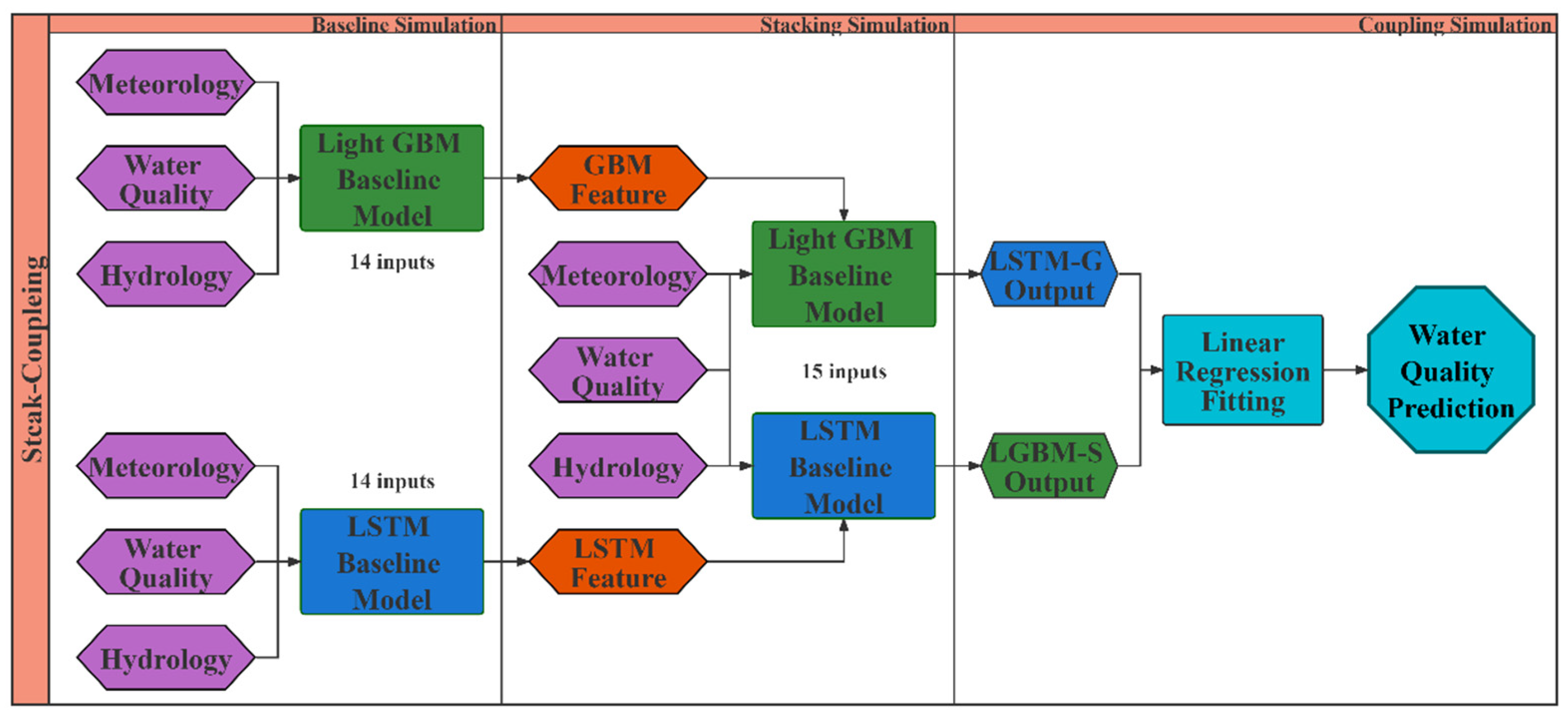
In this study, we attempted to construct a stack coupling machine learning model using the Light GBM and LSTM algorithms. The dataset will be strictly divided into mutually exclusive training and validation sets, with the former used for model fitting and calibration and the latter reserved exclusively for validating the accuracy of trained models. Details could be provided in Section 3.2. As shown in Figure 3, during baseline simulation period, the Light GBM baseline model, 14 input features, including watershed rainfall data, flow data and water quality data, were used to fit the COD concentrations of target section (SHJ) 5 days later.

In order to ensure the accuracy of the model, the hyperparameters of the model were firstly calculated by Bayesian optimization method [69], while 5-fold cross-validation was used to determine the optimal value, and then the hyperparameters were tuned manually based on the Bayesian optimization result [70].

• On the other hand, the Bi-LSTM model was used to construct the LSTM baseline model based on the same dataset, in which the continuous data of the previous 10-day was used to predict the 5-day-later COD concentrations. The training process would be iterated many times to achieve the best fitting effect; while early stopping and dropout mechanisms were also introduced to prevent over-fitting [67,71].
• Then the fitted baseline models would be used to fit and predict the 5-day-later COD concentrations water quality data separately, and the results could be regarded as new features and cross-put into the original baseline model dataset to form the reconstructed baseline model dataset.
• Thus, with the first stack coupling process, two new models would be built and fitted with the same steps as the baseline models, which could be called as LGBM-S model and LSTM-G model, respectively.
• When simulation results from two newly fitted models—each applied to the training and validation datasets, respectively—become available, they would be considered as the input features of the second model coupling based on an SVR with linear kernel (SVR-LK) model, where the final prediction of the 5-day-later concentrations could be calculated.

All those modeling calculations could be implemented through PyTorch 1.10.0 and lightGBM 3.3.2 packages by Python version 3.9, the whole specific workflow of water quality prediction model was as follows:

• The data collected by normalization and data filling is preprocessed.
• Model input variables are selected using correlation coefficient threshold screening and variance inflation factor.
• Two baseline models are built and the prediction values obtained; then the values are added into the baseline models as new input variables to build new models.
• The simple linear model is used to take the predicted value of the new models as new inputs to complete the coupling of the model and obtain the final water quality prediction.

3. Example Application

3.1. Study Area and Data

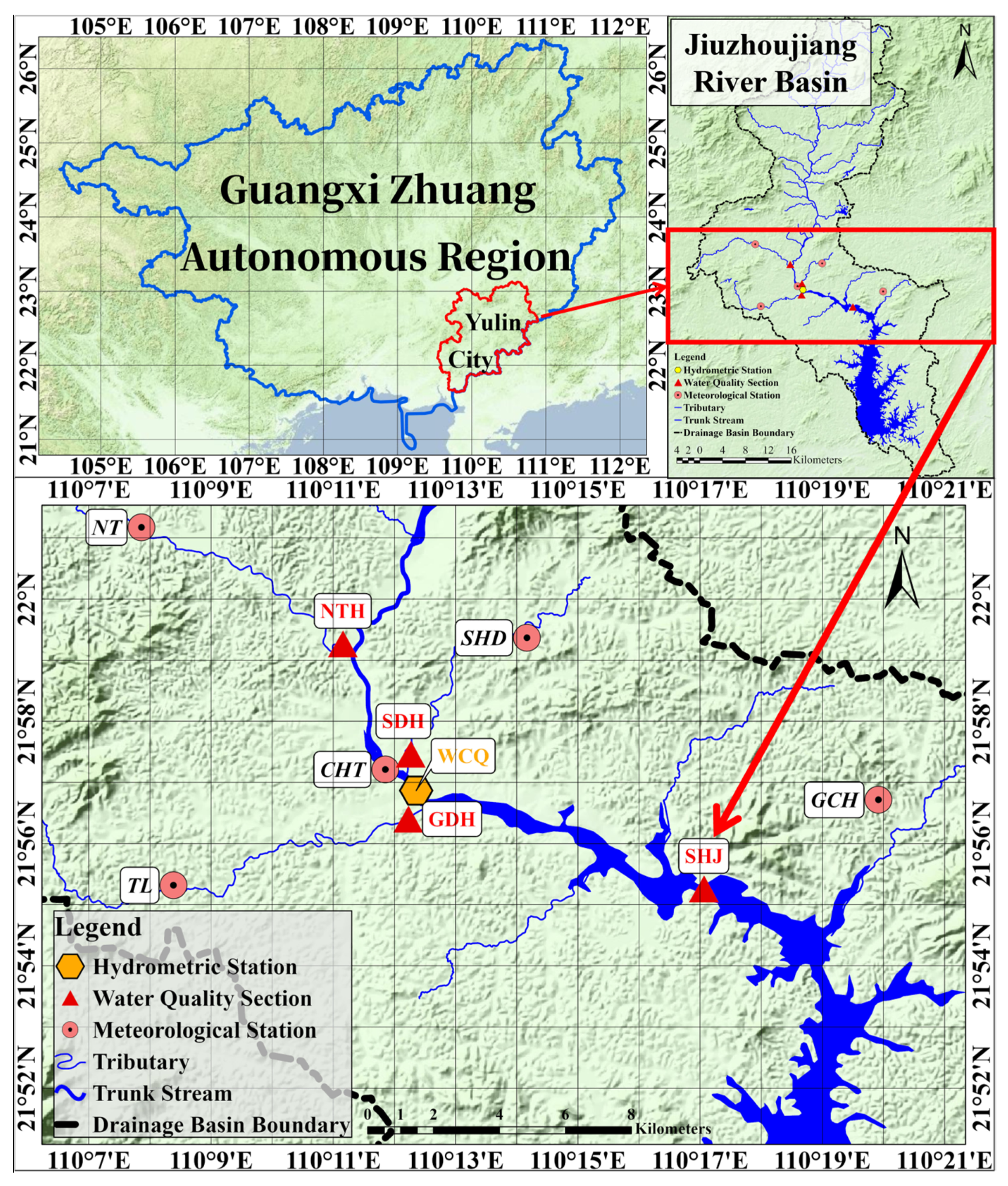
The downstream of Jiuzhoujiang River in Guangxi Zhuang Autonomous Region is considered as a study area in this study, where the river flows into the South China Sea alone across Guangdong Province and Guangxi Region (Figure 4). The river, which is 168 km long and has a total drainage area of 3396 km², originates from Shapo Town, Luchuan County, Yulin City, southeastern Guangxi, flows through Luchuan and Bobai Counties into the Hedi Reservoir at the junction of Guangxi and Guangdong, flows southwest through Zhanjiang City, Guangdong Province, and then enters the North Bay. The trunk stream in Guangxi is 84.8 km long and the total drainage area is 1092 km², which accounts for 32.2% of the total catchment area. Jiuzhoujiang River basin in Guangxi is predominantly forests and agricultural, with forest land, cultivated land and other land use types covering 70.56%, 21.51% and 7.93% of the land area, respectively. Influenced by the subtropical monsoon climate, the study area experiences year-round humidity and heavy rainfall. The precipitation process and the patterns of pollutant migration and transformation are complex. The main pollution sources are livestock and poultry breeding pollution, living source pollution and agricultural non-point source pollution, where fluctuation of river water quality could be greatly affected by the rainfall process. The main pollution indicators are COD, total phosphorus (TP) and ammonia nitrogen (NH₃-N).

Although there are 14 water quality monitoring sections in the study area, with 8 sections on the trunk stream and 6 on the tributaries, only 4 automatic monitoring stations can provide hydro-chemistry data at hourly scales, named NTH, SDH, GDH and SHJ (

Table 1. Basic statistical analysis for automatic water quality monitoring stations.

Sections	Parameters	Unit	Mean	Minimum	Maximum	SD	CV
NTH	WT	°C	24.48	13.94	34.50	4.45	5.51
	pH	—	7.54	6.21	8.80	0.56	13.36
	COD	mg/L	2.52	0.50	7.31	1.44	1.75
SDH	WT	°C	25.14	15.00	32.50	4.58	5.49
	pH	—	7.34	6.08	8.30	0.56	13.12
	COD	mg/L	3.90	0.50	10.04	1.93	2.02
GDH	WT	°C	25.82	11.80	32.10	3.96	6.52
	pH	—	7.47	6.25	8.85	0.52	14.51
	COD	mg/L	5.33	0.50	14.06	2.64	2.02
SHJ	WT	°C	25.82	14.80	34.42	4.75	5.43
	pH	—	7.68	5.30	9.80	0.95	8.12
	COD	mg/L	4.72	2.89	8.69	1.10	4.27

). The three hydrochemical parameters authorized for use in this study are water temperature (WT), pH and COD. These data were obtained from the Department of Ecological Environment of Guangxi. In addition, precipitation data from five meteorological stations at daily scale and flow data from one hydrometric station at monthly scale were also provided (Figure 4,

Table 2. Basic statistical analysis for precipitation data and flow data.

Type	Unit	Stations	Mean	Minimum	Maximum	SD	CV
precipitation	mm	NTR	3.31	0.00	86.00	9.91	0.33
		SDR	2.96	0.00	56.50	8.78	0.34
		CTR	3.26	0.00	80.00	9.97	0.33
		TLR	3.81	0.00	95.00	11.46	0.33
		GCR	3.44	0.00	136.00	11.71	0.29
flow	m3/s	WDH	9.63	2.62	37.4	6.82	1.41

). The data mentioned above can be matched from 21 September 2019 to 10 January 2021. The dataset was preprocessed to ensure consistency: negative values were replaced with zeros, and obvious outliers were flagged as missing. These missing data and unobserved dates were filled using the average of two adjacent days. For periods with more than three consecutive days of missing data, cubic spline interpolation was applied.

All statistical analyses were conducted using SPSS 26 and Python 3.9, with a computing platform of Intel(R) Xeon(R) Silver 4214 CPU @ 2.20 GHz and 64 GB RAM.

3.2. Model Preparation

3.2.1. Selection of Inputs

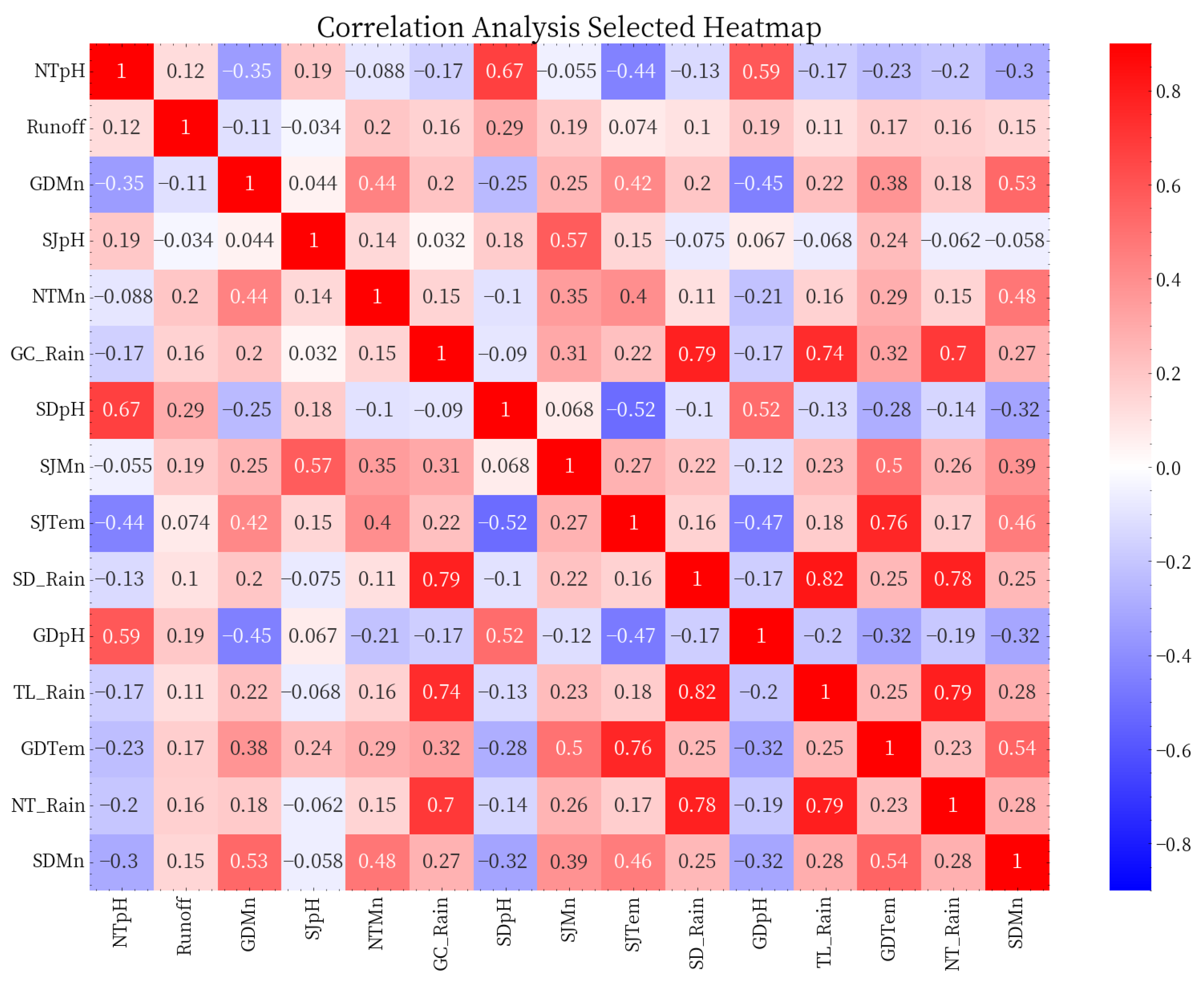
Input selection was carried out by using correlation coefficient threshold screening and variance inflation factor (VIF) methods, respectively, and the results are shown in Figure 5 and

Table 3. The VIF value of the input features.

Feature	VIF	Feature	VIF
NTMn	1.4798	NT_Rain	3.5378
Runoff	1.6709	GDTem	3.8047
GDMn	1.8735	SDpH	4.1896
SJpH	2.0412	TL_Rain	4.6339
SDMn	2.3295	SD_Rain	4.9267
GDpH	2.3306	CT_Rain	6.5421
SJMn	2.7536	SDTem	15.4629
GC_Rain	2.8449	SJTem	16.7376
NTpH	3.3513	NTTem	18.3251

.

As mentioned previously in Section 2.1, the threshold for the correlation coefficient threshold screening was set to 0.85, meaning that only one of the two input variables with a correlation coefficient greater than 0.85 would be retained. The variables finally retained include 15 items such as NTpH, Runoff, GDMn, SJpH, NTMn, GC_Rain, SDpH, SJMn, SJTem, SD_Rain, GDpH, TL_Rain, GDTem, NT_Rain and SDMn. Otherwise, when using the VIF method, the feature should be removed if the VIF value of the feature is >5, as shown in Table 3 [48]. In this case, SJTem was the only extra feature compared to the VIF and threshold screening methods, considering that the value of VIF > 10, still represented a high autocorrelation [47], and SJTem was also eventually removed. As a result, 14 input features were used in this study, and the rainfall data of Chetian and the water temperature data of Shifei River, Shanjiao River and Ningtan River were excluded from the model simulation.

3.2.2. Model Construction

The primary objective of any AI-based model is to select appropriate inputs from an unknown dataset to achieve the desired outputs. Accordingly, the available data were partitioned into strictly independent training and validation sets at a ratio of 70% to 30%, facilitating subsequent training and validation of Baseline models and stack coupling model [32,34,37]. During the training phases, 5-fold cross-validation were employed to maximize calibration accuracy and ensure robust fitting across all models [72]. It should be noted that to prevent the LSTM model from developing lagged predictions and thus becoming a “lazy model” during training, we employed a randomized data splitting approach, consistent with the previous literature [34,73]. To ensure that the LSTM could capture potential temporal dependencies, a 30-day time window was applied prior to any randomized splitting. Within this window, input data were transformed into new feature variables at 10-day intervals, and the dataset was reconstructed accordingly. Furthermore, an alternative LSTM model employing a strict temporal split and sliding window training with the same 10-day interval was also implemented to further verify the credibility of the LSTM baseline model.

Following the construction of the model simulation dataset, we defined search spaces for hyperparameter optimization tailored to each model and employed Bayesian optimization to identify the optimal hyperparameter sets. For the LightGBM algorithm, the specific hyperparameters evaluated are listed in

Table 4. Hyperparameter search space for Light GBM algorithm.

Category	Hyperparameter	Search Spaces
Core Control	boosting_type	GBDT (Fixed)
	objective	regression (Fixed)
	n_estimators	[1000, 5000]
	learning_rate	[0.001, 0.1]
Tree Structure	num_leaves	[2, 100]
	max_depth	[2, 20]
	max_bin	[2, 20]
	min_child_samples	[0.01, 1]
	colsample_bytree	[0.01, 1]
Others	reg_alpha	[0.001, 1]
	reg_lambda	[0.001, 1]
	stopping_rounds	500 (Fixed)
	eval_metric	RMSE (Fixed)

.

Similarly, the specific hyperparameters evaluated for the LSTM algorithm are listed in

Table 5. Hyperparameter search space for LSTM algorithm.

Category	Hyperparameter	Search Spaces
Model Architecture	hidden Size	[32, 256]
	number of Layers	[1, 2]
Training Process	epochs	[1000, 5000]
	learning_rate	[0.00001, 0.01]
	batch size	[64, 512]
	weight_decay	[0.00001, 0.01]
	optimizer	Adam (Fixed)
Regularization	L1_reg	[0.001, 1]
	dropout rate	[0.01, 0.3]
	stopping_rounds	500 (Fixed)
	Loss_metric	RMSE (Fixed)

.

3.3. Prediction of Water Quality

3.3.1. Simulation Results of Baseline Models and Stack Coupling Model

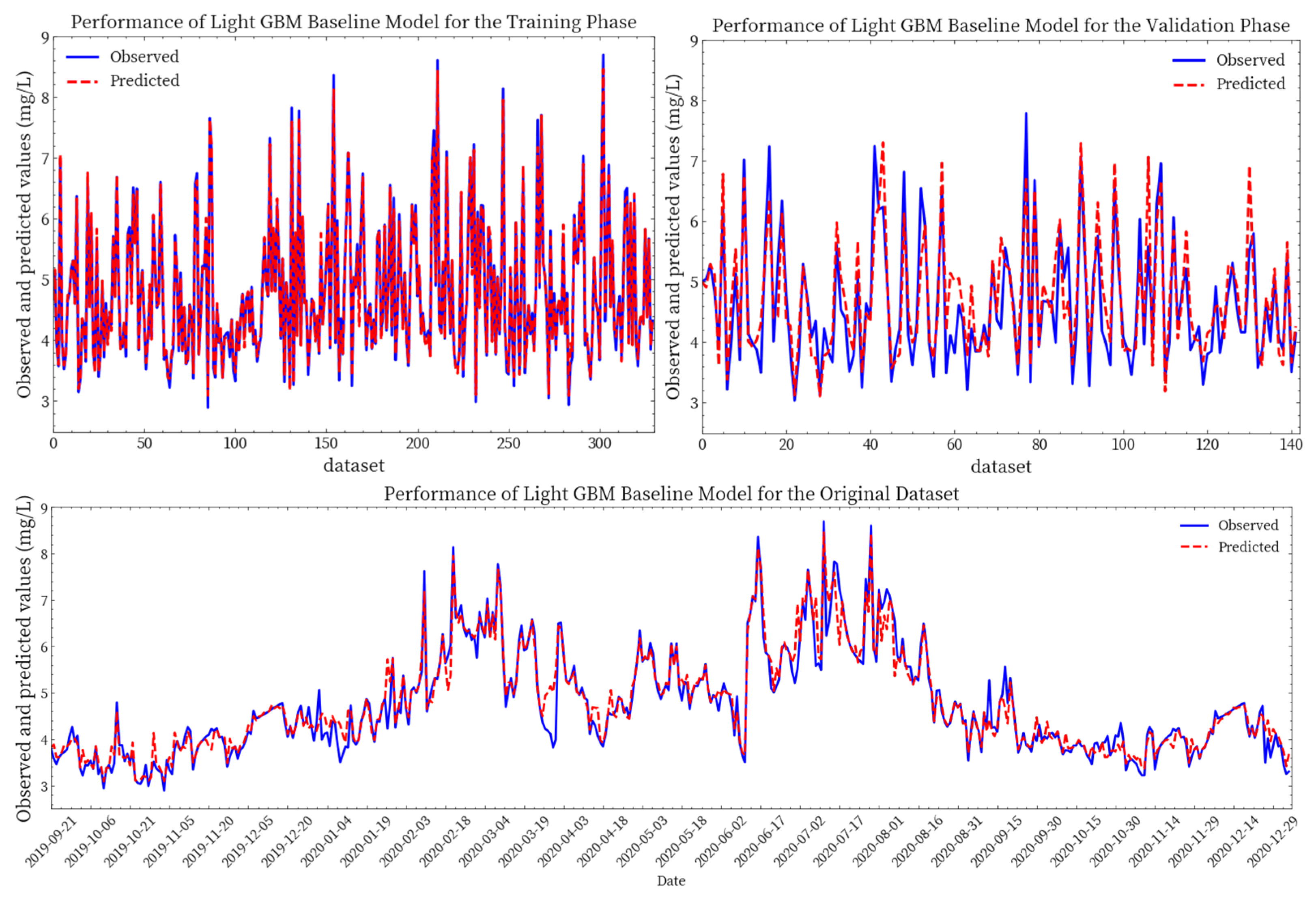
As mentioned before, in Light GBM baseline model simulation, 70% of the original dataset was selected randomly as the training dataset, while the remaining 30% was used as the validation dataset. After the model was fitted, the training dataset, validation dataset and original dataset were simulated in the fitted model. The results of the simulations are as follows (Figure 6).

As shown in

Table 6. Performance metrics of the Light GBM baseline model (where CC means correlation coefficient between observed data and predicted data).

	NSE	Adj. R2	RMSE (mg/L)	MAPE (%)	CC
Overall	0.935	0.933	0.282	3.496	0.967
Training	0.993	0.993	0.195	1.468	0.996
Validation	0.761	0.736	0.492	8.153	0.886

, during the simulation of the Light GBM baseline model, the total NSE and RMSE of the original dataset were 0.935 and 0.282 mg/L, respectively, while the NSE and RMSE of the training phase were 0.993 and 0.195 mg/L, respectively. And the NSE and RMSE of the validation phase were 0.761 and 0.492 mg/L, respectively. The difference in NSE and RMSE between training phase and validation phase was 0.232 and −0.297 mg/L, respectively.

Similarly, in the LSTM baseline model simulation, 70% of the original dataset was selected randomly as the training dataset, while the remaining 30% was used as the validation dataset. After the model was fitted, the training dataset, validation dataset and original dataset were simulated in the fitted model. The results of the simulations are as follows (Figure 7).

As shown in

Table 7. Performance metrics of the LSTM baseline model (where CC means correlation coefficient between observed data and predicted data).

	NSE	Adj. R2	RMSE (mg/L)	MAPE (%)	CC
Overall	0.842	0.837	0.439	6.289	0.920
Train	0.875	0.870	0.401	6.470	0.938
Validation	0.738	0.709	0.525	6.890	0.868

, during the simulation of LSTM baseline model, the total NSE and RMSE of the original dataset were 0.842 and 0.439 mg/L, respectively, while the NSE and RMSE in the training phase were 0.875 and 0.401 mg/L, respectively. And the NSE and RMSE during the validation phase were 0.738 and 0.525 mg/L, respectively. The difference in NSE and RMSE between training phase and validation phase was 0.037 and −0.124 mg/L, respectively.

Moreover, the LSTM model simulation results (Figure A1) based on LSTM model employing a strict temporal split can be found in the Appendix A, where we compare the performance metrics (

Table A1. Performance metrics of LSTM model with a strict temporal split (where CC means correlation coefficient between observed data and predicted data).

	NSE	Adj. R2	RMSE (mg/L)	MAPE (%)	CC
Overall	0.841	0.837	0.479	5.618	0.931
Train	0.842	0.836	0.409	5.944	0.933
Validation	0.735	0.700	0.422	5.733	0.891

) of two LSTM models and further verify the data distribution characteristics of two prediction results (

Table A2. Kruskal–Wallis test results of LSTM model with a strict temporal split.

Models	p-Value	Test Statistic	Alpha Level	H0
LSTM model with a strict temporal split	0.188	1.733	0.05	Accept

).

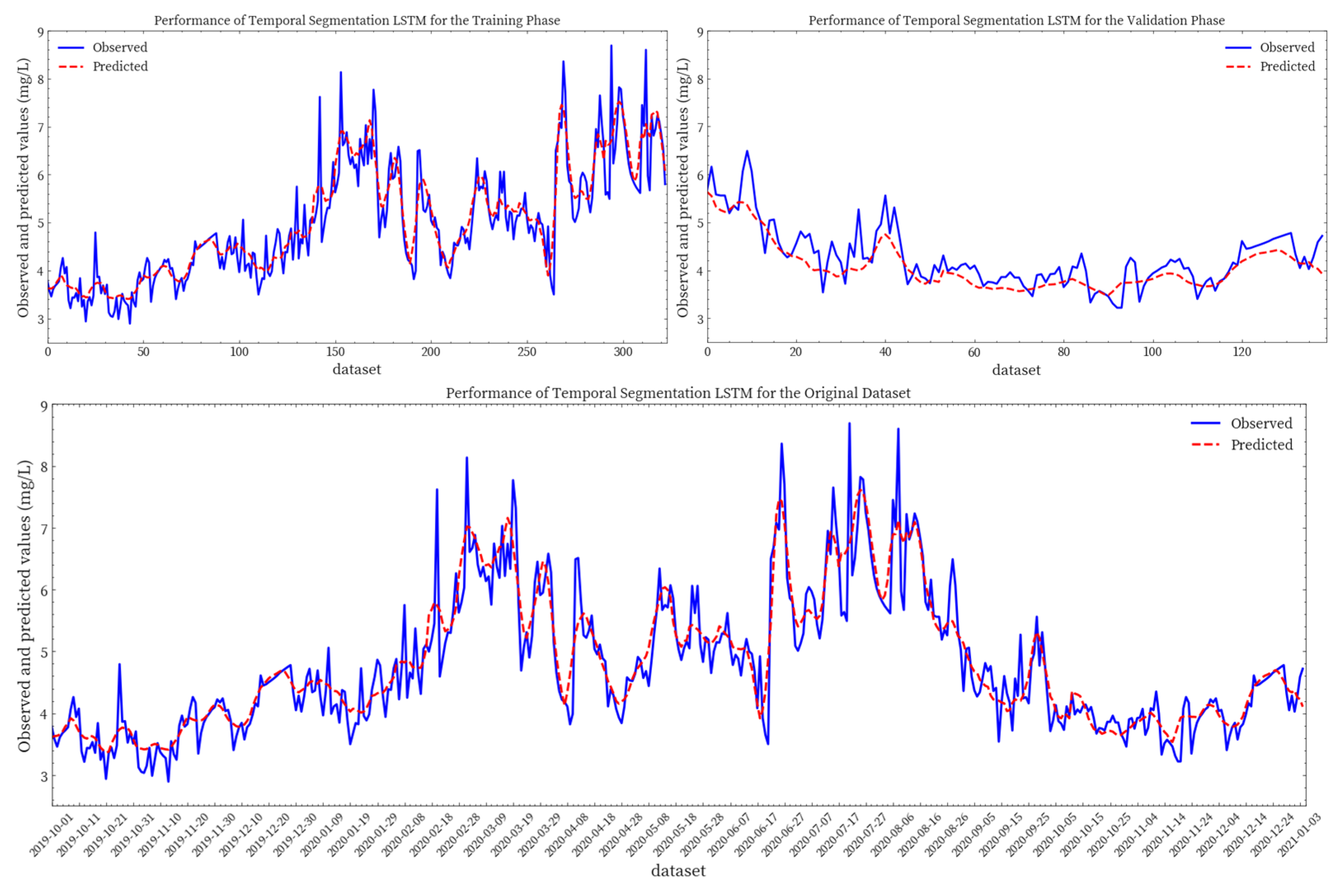
After two steps of model coupling, the final prediction of COD concentration was carried out by simulating the output of LGBM-S model and LSTM-G model with the stack coupling model, which was called the SVR-LK model. After the model was fitted, the training dataset, validation dataset and original dataset were simulated in the fitted model, respectively. The results of the simulations were as follows (Figure 8).

As shown in

Table 8. Performance metrics of the stack coupling (SVR-LK) model (where CC means correlation coefficient between observed data and predicted data).

	NSE	Adj. R2	RMSE (mg/L)	MAPE (%)	CC
Overall	0.881	0.881	0.380	5.404	0.939
Train	0.904	0.903	0.342	5.052	0.951
Validation	0.829	0.826	0.455	6.224	0.912

, during the simulation of stack coupling model (SVR-LK), the total NSE and RMSE of the original dataset were 0.881 and 0.380 mg/L, respectively, while the NSE and RMSE in the training phase were 0.904 and 0.342 mg/L, respectively. And the NSE and RMSE during the validation phase were 0.829 and 0.455 mg/L, respectively. The difference in NSE and RMSE between training phase and validation phase was 0.75 and −0.113 mg/L, respectively.

3.3.2. Validation Performance Between All the Five Models

Prior to model performance comparison, the Kruskal–Wallis test was conducted to assess whether the predictions from those five models (Light GBM, LSTM, LGBM-S, LSTM-G and SVR-LK models) and the experimentally measured data originate from the same distribution, thereby evaluating the robustness of the models [74]. As shown in

Table 9. Kruskal–Wallis test results of the five models.

Models	p-Value	Test Statistic	Alpha Level	H0
Light GBM	0.144	2.134	0.05	Accept
LSTM	0.234	1.419	0.05	Accept
LGBM-S	0.654	0.201	0.05	Accept
LSTM-G	0.561	0.337	0.05	Accept
SVR-LK	0.773	0.121	0.05	Accept

, the results from all five models fail to reject the null hypothesis (H₀), indicating no statistically significant difference between the predicted and observed data. Moreover, the SVR-LK model could be considered to be more robust than other approaches.

Figure 9A–E shows scatter plots between the observed and predicted values of the Light GBM, LSTM, LGBM-S, LSTM-G and SVR-LK in the validation phase. It is clear that a closeness agreement between the observed and predicted values was attained. The overall comparison of the computational intelligence techniques indicates the satisfactory performance accuracy of Light GBM, LSTM, LGBM-S, LSTM-G and SVR-LK models in validation phase, which can be justified by considering the correlation coefficient (

Table 10. Performance metrics of the five models in validation.

Models	NSE	Adj. R2	RMSE (mg/L)	MAPE (%)
Light GBM	0.761	0.736	0.492	8.153
LSTM	0.738	0.709	0.525	6.890
LGBM-S	0.778	0.802	0.457	6.041
LSTM-G	0.794	0.769	0.492	6.472
SVR-LK	0.829	0.826	0.452	6.224

). The values of correlation coefficient higher than 0.70 are considered acceptable; thus, the results of all models are acceptable with each value of correlation coefficient higher than 0.85 [49,75].

These metrics, which incorporate both error measurements and goodness-of-fit criteria, serve as effective indicators of model performance.

4. Discussion

4.1. Improvement of Water Quality Prediction Model of Stack Coupling Model

As shown in Table 10, both Light GBM and LSTM models could predict the future short-term water quality of the river with high accuracy. The NSE of both models for the validation phase was above 0.75, while the MAPE was below 10%. This suggested that the simulation results of a single machine learning algorithm in the study area were already reliable. However, these results also implied that using only one algorithm was not sufficient to further enhance the predictive accuracy of the model. Considering the basic principles of the two algorithms, the Light GBM simulation process assumed a one-to-one response relationship between future water quality and input features on time-series data, which might not capture the stacking lag effect on time-series data [28,55,76,77]. Likewise, LSTM might face some challenges in detecting potential relationships between data with different spatial attributes, leading to local optima [67,68,78]. Therefore, it was worthwhile to couple the two models using a stacking approach. To the best of our knowledge, there have been few attempts to address those problems by coupling the gradient boost machine and LSTM algorithm [18,62]. Thus, we attempted to stack the LSTM simulation results and LGB simulation results as new variables into the other model. The results indicated that the performance of both new models was very similar, with NSE of both new models reaching 0.8 and MAPE dropping to around 6%. Therefore, it was hard to draw from previous experience to further analyze whether the LGBM-S model containing the prediction results of the LSTM baseline model or the LSTM-G model containing the results of the Light GBM baseline model was the optimal choice. The model performance evaluation results showed that both prediction models were accurate and reliable. However, due to the existence of residuals, their predicted values deviated from the observed values to some degree. To minimize this deviation as much as possible, we applied an SVR-LK model to fit the prediction results of the two models. The results indicated that the NSE further increased, while the MAPE further decreased. As a summary, Figure 10 shows five performance metrics (NSE, Adj. R², RMSE and MAPE) for all five models involved in the study. The NSE of validation datasets of five models increased with the increase in model stacking times; i.e., through stack coupling steps, the final model could reduce variance. Likewise, the RMSE results suggest that the bias of the stacked coupling model was also minimal. Moreover, compared to the baseline model, the difference between various evaluation indicators of the final model in training and validation datasets was also minimal. This suggests that the stack coupling model had high accuracy and robustness and had good generalization value [62,79,80].

However, the modeling framework developed in this study still presents certain limitations, which can be summarized as follows: First, the performance of the model relies heavily on large volumes of accurate observational data. When data availability is limited, the model is prone to overfitting or may degenerate into inert models when dealing with small sample sizes or numerous outliers. Second, the fundamental principles underlying the LightGBM and LSTM algorithms—which form the spatiotemporal data mining engine—are fundamentally distinct, further compromising the interpretability of the integrated model and complicating the identification of driving factors behind aquatic environmental changes. As discussed in later sections, investigations into time-lag effects and driving factors remain based on baseline models. These limitations warrant future work focused on expanding the ensemble with physically based models as base learners and incorporating explainable AI (XAI) techniques to enhance interpretability.

4.2. Advantages and Contributions of the Baseline Model in Water Quality Prediction

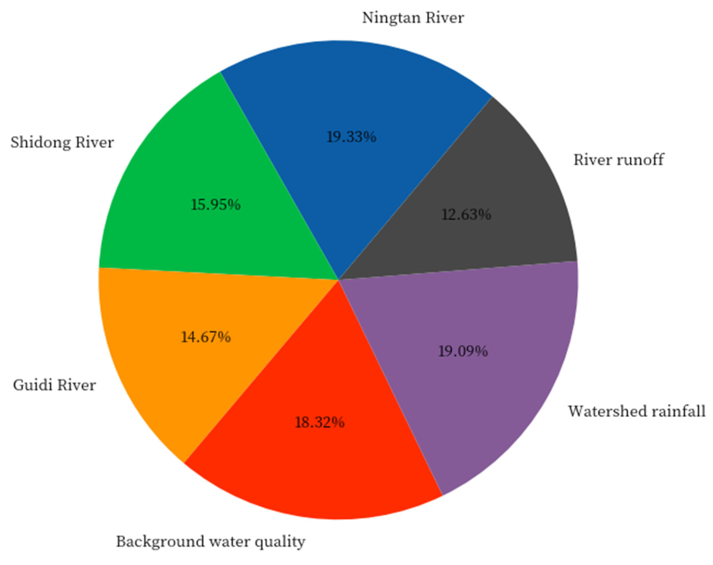
The variation in river water quality was mainly influenced by the nonlinear superposition between the background pollutant concentration and the input pollutant concentration, which could have been mainly determined by the amount of water and pollutants input from the upstream and rainfall in the watershed [5,7]. It was essential to extract more reasonable water quality impact factors in water quality prediction and identify their temporal stacking lag effect. In this article, the Light GBM baseline model was used to find the main influencing factors and identify driving contributions. Figure 11 indicates the driving factors and the proportion of their contributions to the variation in COD concentration at SHJ station after consolidation and simplification. As shown in the figure, watershed rainfall, background water quality, river runoff, and the water quality of Ningtan River, Shidong River and Guidi River were the main driving elements at SHJ station. The contribution of each factor was relatively consistent, with the proportion ranging from 12% to 20%. Among them, the water quality of Ningtan River, watershed rainfall and background water quality of SHJ station contributed the most, contributing 19.3%, 19.1% and 18.3%, respectively, which was in line with the pollution status of Jiuzhoujiang River basin. It should be noted that before affecting the water quality of the research station, the concentration of pollutants in the upstream was already influenced by the watershed rainfall and the non-point source pollutants that entered the river. Therefore, how to accurately separate the contribution of rainfall in the basin still requires further research.

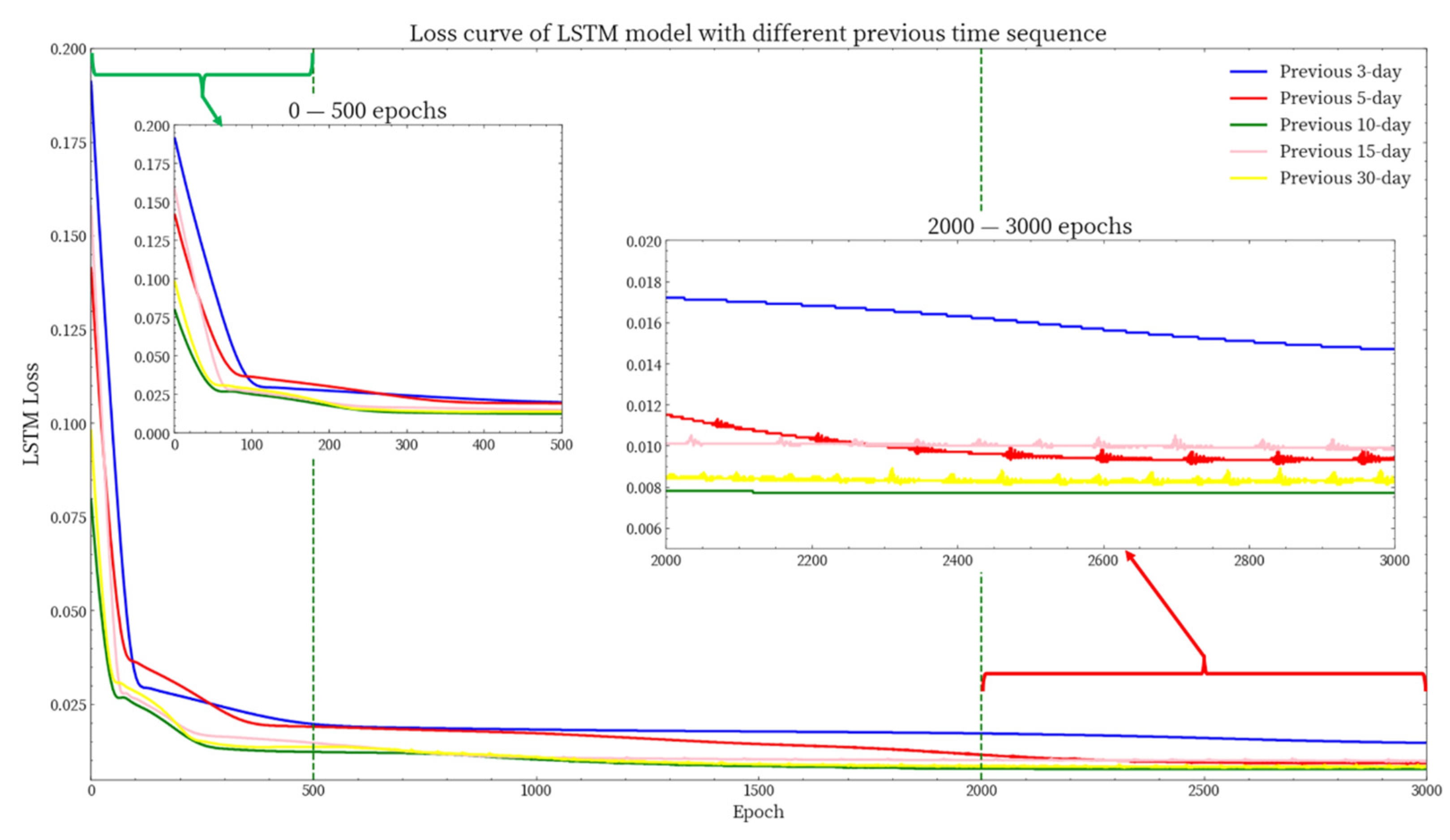
As a special recurrent neural network, there are three kinds of gates with memory cells inside (i.e., input, forget, and output) in LSTM. It maintains a persistent state that can be passed between different neurons to determine whether information should be passed or forgotten. Based on this structure, the water quality prediction model using LSTM algorithm could fit the nonlinear effects such as time stacking and lagging of the previous water quality series on future water quality to improve the accuracy of prediction [67,81]. To obtain the range of time-series data sequence which could have been the most important influence on the lag stacking of water quality variables in the future, the LSTM model was used to simulate the response relationship between the previous 3-day, 5-day, 10-day, 15-day and 30-day data series and the 5-days-later water quality, and the results are shown in Figure 12. Obviously, after 3000 epochs of iterative learning, the loss function values of 10-day and 30-day previous scenarios were the best. Since the prediction model mainly targeted short-term water quality changes and the 30-day range might average the data features, we selected the previous 10-day series for use in the model construction [30]. This also confirmed that the influence period of the previous sequence data on the future water quality should be 10–15 days [82]. It should be noted that since the previous sequence time-series data included water quality, rainfall and runoff, the stacking lag range of different types of data might also differ. Therefore, the lag effect of separating different types of data is also worth studying further.

4.3. Uncertainty Analysis

The simulation of different data by prediction models might have considerable uncertainty, which could have a significant impact on the universality and stability of the model [34,83,84]. To further evaluate the performance of the model, 2000 different training and validation datasets were constructed by randomly sampling the study dataset. Then, baseline models and the stack coupling model was applied to evaluate the impact of dataset uncertainty on model performance. The comparison results with the baseline model RMSE are shown in

Table 11. Uncertainty evaluation compared with baseline models and coupling model.

Models	Min RMSE	Max RMSE	Medium	Epoch
Stack Coupling model	0.122 mg/L	0.542 mg/L	0.389 mg/L	2000 times
Light GBM baseline model	0.206 mg/L	0.677 mg/L	0.454 mg/L	2000 times
LSTM baseline model	0.278 mg/L	0.746 mg/L	0.532 mg/L	2000 times

. Results showed the performance of the stack coupling model (multiple tests of RMSE range 0.12~0.54 mg/L) compared to the separate LightGBM baseline model (multiple test RMSE range 0.2~0.68 mg/L) and LSTM baseline model (multiple test RMSE range 0.28~0.75 mg/L). The stability of the model has increased by 15% to 40%. Thus, the short-term prediction method based on the stack coupling model had high predictive accuracy and stability. The above analysis was based on considering only the uncertainty of input data and model structures. In addition to this, other sources of uncertainty, such as measurement errors, data processing, and insufficient sampling, were all important issues in river water quality modeling.

5. Conclusions

To enhance the short-term prediction accuracy of river water quality and extract the influence factors of water quality change, we applied a two-step stack coupling model in this study. That is, we stacked the Light GBM model and LSTM model by an SVR-LK model to investigate the short-term water quality prediction in Jiuzhoujiang River basin. The result was as follows:

(1)

Both the baseline models (LightGBM and LSTM) demonstrated high accuracy in predicting short-term river water quality and exhibited a considerable robustness. The NSE of both models for the validation phase was above 0.75, while the MAPE was below 10%. Furthermore, both “process models” (LGBM-S and LSTM-G) demonstrated modest but consistent improvements in accuracy compared to the baseline model. This suggests that the process models capture information not adequately represented in the baseline simulations, such as spatial dependencies and temporal lag effects.

(2)

A Light GBM with Bayesian optimization baseline model was built to predict the river water quality mainly focusing on potential relationships between data with different spatial attributes. The result indicated that the main driving factors of the variation in study area were upstream from Ningtan River, watershed rainfall and background water quality.

(3)

A LSTM with bidirectional connection baseline model was built to predict the river water quality mainly focusing on the stacking lag effect of time-series data. The result indicated that the short-term river water quality was affected by the stacking lag of the time-series data of the previous 10–15 days.

(4)

Owing to the presence of residuals, the predictions deviate somewhat from the observed values. To minimize this deviation and enhance the accuracy of water quality prediction, the simulation results of the two models are recalculated as input variables for one another and then coupled through an SVR-LK model to obtain the final predicted value. It was found that the accuracy of the stack coupling model had increased by 8~12% and the stability of the coupling model had increased by 15–40%. This outcome provides a robust technical foundation for future basin-wide water quality forecasting, early-warning, and real-time environmental management in Guangxi. The approach has already been extended to the Yellow River Basin and the Beijing-Tianjin-Hebei region.

(5)

The modeling framework established in this study remains limited in terms of data requirements and physical interpretability. Therefore, a promising direction for future work involves expanding the ensemble to include physics-based models as base learners, while integrating explainable AI (XAI) techniques to enhance transparency and mechanistic insight.

References

1. Khalil, B.; Ouarda, T.B.M.J.; St-Hilaire, A.; Chebana, F. A statistical approach for the rationalization of water quality indicators in surface water quality monitoring networks. J. Hydrol. 2010, 386, 173–185. [Google Scholar] [CrossRef]
2. Grabowski, R.C.; Gurnell, A.M. Hydrogeomorphology—Ecology interactions in river systems. River Res. Appl. 2016, 32, 139–141. [Google Scholar] [CrossRef]
3. Singh, A.P.; Dhadse, K.; Ahalawat, J. Managing water quality of a river using an integrated geographically weighted regression technique with fuzzy decision-making model. Environ. Monit. Assess. 2019, 191, 378. [Google Scholar] [CrossRef]
4. Vörösmarty, C.J.; McIntyre, P.B.; Gessner, M.O.; Dudgeon, D.; Prusevich, A.; Green, P.; Glidden, S.; Bunn, S.E.; Sullivan, C.A.; Liermann, C.R.; et al. Global threats to human water security and river biodiversity. Nature 2010, 467, 555–561. [Google Scholar] [CrossRef]
5. Cheng, H.; Hu, Y.; Zhao, J. Meeting china’s water shortage crisis: Current practices and challenges. Environ. Sci. Technol. 2009, 43, 240–244. [Google Scholar] [CrossRef]
6. Tripathi, M.; Singal, S.K. Use of principal component analysis for parameter selection for development of a novel water quality index: A case study of river ganga india. Ecol. Indic. 2019, 96, 430–436. [Google Scholar] [CrossRef]
7. Uddin, M.G.; Nash, S.; Rahman, A.; Olbert, A.I. A comprehensive method for improvement of water quality index (WQI) models for coastal water quality assessment. Water Res. 2022, 219, 118532. [Google Scholar] [CrossRef]
8. Ahmed, A.N.; Othman, F.B.; Afan, H.A.; Ibrahim, R.K.; Fai, C.M.; Hossain, M.S.; Ehteram, M.; Elshafie, A. Machine learning methods for better water quality prediction. J. Hydrol. 2019, 578, 124084. [Google Scholar] [CrossRef]
9. Antanasijević, D.; Pocajt, V.; Povrenovic, D.; Peric-Grujic, A.; Ristic, M. Modelling of dissolved oxygen content using artificial neural networks: Danube River, North Serbia, case study. Environ. Sci. Pollut. Res. 2013, 20, 9006–9013. [Google Scholar] [CrossRef] [PubMed]
10. Tchobanoglous, G.; Schroeder, E.E. Water Quality: Characteristics, Modeling, Modification; Addison-Wesley Publishing Co., Ltd.: Reading, MA, USA, 1985; p. 704. [Google Scholar]
11. Mohtar, W.H.M.W.; Maulud, K.N.A.; Muhammad, N.S.; Sharil, S.; Zaher Mundher, Y. Spatial and temporal risk quotient based river assessment for water resources management. Environ. Pollut. 2019, 248, 133–144. [Google Scholar] [CrossRef] [PubMed]
12. Reichert, P.; Borchardt, D.; Henze, M.; Rauch, W.; Shanahan, P.; Somlyody, L.; Vanrolleghem, P. River Water Quality Model No 1; IWA Publishing: London, UK, 2001. [Google Scholar]
13. Chapra, S.; Pellettier, G. QUAL2K: A Modeling Framework for Simulating River and Stream Water Quality; Tufts University: Medford, MA, USA, 2003. [Google Scholar]
14. Wool, T.A.; Ambrose, R.B.; Martin, J.L.; Comer, E.A. Water Quality Analysis Simulation Program (WASP) Version 6.0 DRAFT: User’s Manual; US Environmental Protection Agency: Athens, GA, USA, 2006.
15. Jothiprakash, V.; Magar, R.B. Multi-time-step ahead daily and hourly intermittent reservoir inflow prediction by artificial intelligent techniques using lumped and distributed data. J. Hydrol. 2012, 450, 293–307. [Google Scholar] [CrossRef]
16. Meybeck, M. Global analysis of river systems: From Earth system controls to Anthropocene syndromes. Philos. Trans. R. Soc. Lond. Ser. B Biol. Sci. 2003, 358, 1935–1955. [Google Scholar] [CrossRef]
17. Hey, T. The Fourth Paradigm—Data-Intensive Scientific Discovery, IMCW 2012; Springer: Berlin/Heidelberg, Germany, 2012; p. 1. [Google Scholar]
18. Tiyasha, T. Tung, T.M.; Yaseen, Z.M. A survey on river water quality modelling using artificial intelligence models: 2000–2020. J. Hydrol. 2020, 585, 124670. [Google Scholar] [CrossRef]
19. Turan, M.E.; Yurdusev, M.A. River flow estimation from upstream flow records by artificial intelligence methods. J. Hydrol. 2009, 369, 71–77. [Google Scholar] [CrossRef]
20. Quej, V.H.; Almorox, J.; Arnaldo, J.A.; Saito, L. ANFIS, SVM and ANN soft-computing techniques to estimate daily global solar radiation in a warm sub-humid environment. J. Atmos. Sol.-Terr. Phy. 2017, 155, 62–70. [Google Scholar] [CrossRef]
21. Huang, W.R.; Foo, S. Neural network modeling of salinity variation in Apalachicola River. Water Res. 2002, 36, 356–362. [Google Scholar] [CrossRef] [PubMed]
22. Heddam, S. Multilayer perceptron neural network-based approach for modeling phycocyanin pigment concentrations: Case study from lower Charles River buoy, USA. Environ. Sci. Pollut. Res. 2016, 23, 17210–17225. [Google Scholar] [CrossRef]
23. Gebler, D.; Wiegleb, G.; Szoszkiewicz, K. Integrating river hydromorphology and water quality into ecological status modelling by artificial neural networks. Water Res. 2018, 139, 395–405. [Google Scholar] [CrossRef]
24. Yan, H.; Zou, Z.; Wang, H. Adaptive neuro fuzzy inference system for classification of water quality status. J. Environ. Sci. 2010, 22, 1891–1896. [Google Scholar] [CrossRef]
25. Ahmed, A.A.M.; Syed Mustakim Ali, S. Application of adaptive neuro-fuzzy inference system (ANFIS) to estimate the biochemical oxygen demand (BOD) of Surma River. J. King Saud Univ.-Eng. Sci. 2017, 29, 237–243. [Google Scholar] [CrossRef]
26. Kamyab-Talesh, F.; Mousavi, S.-F.; Khaledian, M.; Yousefi-Falakdehi, O.; Norouzi-Masir, M. Prediction of Water Quality Index by Support Vector Machine: A Case Study in the Sefidrud Basin, Northern Iran. Water Resour. 2019, 46, 112–116. [Google Scholar] [CrossRef]
27. Ho, J.Y.; Afan, H.A.; El-Shafie, A.H.; Koting, S.B.; Mohd, N.S.; Jaafar, W.Z.B.; Hin, L.S.; Malek, M.A.; Ahmed, A.N.; Mohtar, W.H.M.W.; et al. Towards a time and cost effective approach to water quality index class prediction. J. Hydrol. 2019, 575, 148–165. [Google Scholar] [CrossRef]
28. Maier, P.M.; Keller, S. Machine Learning Regression on Hyperspectral Data to Estimate Multiple Water Parameters. In Proceedings of the 9th Workshop on Hyperspectral Image and Signal Processing: Evolution in Remote Sensing (WHISPERS), Amsterdam, The Netherlands, 23–26 September 2018. [Google Scholar]
29. Najah, A.A.; El-Shafie, A.; Karim, O.A.; Jaafar, O. Water quality prediction model utilizing integrated wavelet-ANFIS model with cross-validation. Neural Comput. Appl. 2012, 21, 833–841. [Google Scholar] [CrossRef]
30. Jin, T.; Cai, S.B.; Jiang, D.X.; Liu, J. A data-driven model for real-time water quality prediction and early warning by an integration method. Environ. Sci. Pollut. Res. 2019, 26, 30374–30385. [Google Scholar] [CrossRef]
31. Faruk, D.O. A hybrid neural network and ARIMA model for water quality time series prediction. Eng. Appl. Artif. Intell. 2010, 23, 586–594. [Google Scholar] [CrossRef]
32. Rajaee, T.; Khani, S.; Ravansalar, M. Artificial intelligence-based single and hybrid models for prediction of water quality in rivers: A review. Chemom. Intell. Lab. Syst. 2020, 200, 103978. [Google Scholar] [CrossRef]
33. Usman, A.G.; Işik, S.; Abba, S.I. A Novel Multi-model Data-Driven Ensemble Technique for the Prediction of Retention Factor in HPLC Method Development. Chromatographia 2020, 83, 933–945. [Google Scholar] [CrossRef]
34. Antanasijević, D.; Pocajt, V.; Peric-Grujic, A.; Ristic, M. Modelling of dissolved oxygen in the Danube River using artificial neural networks and Monte Carlo Simulation uncertainty analysis. J. Hydrol. 2014, 519, 1895–1907. [Google Scholar] [CrossRef]
35. Jiawei, H.; Micheline, K.; Jian, P. 3-Data Preprocessing. In Data Mining: Concepts and Techniques, 3rd ed.; Jiawei, H., Micheline, K., Jian, P., Eds.; Morgan Kaufmann: Boston, MA, USA, 2012; pp. 83–124. ISBN 978-0-12-381479-1. [Google Scholar] [CrossRef]
36. Abba, S.I.; Hadi, S.J.; Sammen, S.S.; Salih, S.Q.; Abdulkadir, R.A.; Pham, Q.B.; Yaseen, Z.M. Evolutionary computational intelligence algorithm coupled with self-tuning predictive model for water quality index determination. J. Hydrol. 2020, 587, 124974. [Google Scholar] [CrossRef]
37. Abba, S.I.; Abdulkadir, R.A.; Saad Sh, S.; Quoc Bao, P.; Lawan, A.A.; Parvaneh, E.; Anurag, M.; Nadhir, A.-A. Integrating feature extraction approaches with hybrid emotional neural networks for water quality index modeling. Appl. Soft Comput. 2022, 114, 108036. [Google Scholar] [CrossRef]
38. Zebari, R.; Abdulazeez, A.; Zeebaree, D.; Zebari, D.; Saeed, J. A Comprehensive Review of Dimensionality Reduction Techniques for Feature Selection and Feature Extraction. J. Appl. Sci. Technol. Trends 2020, 1, 56–70. [Google Scholar] [CrossRef]
39. Aremu, O.O.; Hyland-Wood, D.; McAree, P.R. A machine learning approach to circumventing the curse of dimensionality in discontinuous time series machine data. Reliab. Eng. Syst. Saf. 2020, 195, 106706. [Google Scholar] [CrossRef]
40. Wang, L.; Jiang, S.; Jiang, S. A feature selection method via analysis of relevance, redundancy, and interaction. Expert Syst. Appl. 2021, 183, 115365. [Google Scholar] [CrossRef]
41. Myers, J.; Well, A.; Lorch, R. Between-Subjects Designs: Several Factors. In Research Design and Statistical Analysis, 3rd ed.; Routledge: New York, NY, USA, 2010; ISBN 9780203726631. [Google Scholar] [CrossRef]
42. Elith, J.; Graham, C.; Anderson, R.; Dudík, M.; Ferrier, S.; Guisan, A.; Hijmans, R.; Huettmann, F.; Leathwick, J.; Lehmann, A.; et al. Novel methods improve prediction of species’ distributions from occurrence data. Ecography 2006, 29, 129–151. [Google Scholar] [CrossRef]
43. Dormann, C.; Elith, J.; Bacher, S.; Buchmann, C.; Carl, G.; Carré, G.; Marquéz, J.; Gruber, B.; Lafourcade, B.; Leitao, P.; et al. Collinearity: A review of methods to deal with it and a simulation study evaluating their performance. Ecography 2013, 36, 27–46. [Google Scholar] [CrossRef]
44. Kasraei, B.; Schmidt, M.G.; Zhang, J.; Bulmer, C.E.; Filatow, D.S.; Arbor, A.; Pennell, T.; Heung, B. A framework for optimizing environmental covariates to support model interpretability in digital soil mapping. Geoderma 2024, 445, 116873. [Google Scholar] [CrossRef]
45. Salmerón, R.; García, C.; García, J. Variance Inflation Factor and Condition Number in multiple linear regression. J. Stat. Comput. Simul. 2018, 88, 2365–2384. [Google Scholar] [CrossRef]
46. Maier, H.R.; Jain, A.; Dandy, G.C.; Sudheer, K.P. Methods used for the development of neural networks for the prediction of water resource variables in river systems: Current status and future directions. Environ. Modell. Softw. 2010, 25, 891–909. [Google Scholar] [CrossRef]
47. Kroll, C.N.; Song, P. Impact of multicollinearity on small sample hydrologic regression models. Water Resour. Res. 2013, 49, 3756–3769. [Google Scholar] [CrossRef]
48. Demir, V.; Citakoglu, H. Forecasting of solar radiation using different machine learning approaches. Neural Comput. Appl. 2023, 35, 887–906. [Google Scholar] [CrossRef]
49. Legates, D.R.; McCabe, G.J. Evaluating the use of “goodness-of-fit” measures in hydrologic and hydroclimatic model validation. Water Resour. Res. 1999, 35, 233–241. [Google Scholar] [CrossRef]
50. Hastie, T.; Tibshirani, R.; Friedman, J.H. Boosting and Additive Trees. In The Elements of Statistical Learning: Data Mining, Inference, and Prediction, 2nd ed.; Springer: New York, NY, USA, 2009; Volume 10, pp. 337–384. [Google Scholar]
51. Natekin, A.; Knoll, A. Gradient boosting machines, a tutorial. Front. Neurorobot. 2013, 7, 21. [Google Scholar] [CrossRef]
52. Alsabti, K.; Ranka, S.; Singh, V. CLOUDS: A Decision Tree Classifier for Large Datasets. In Proceedings of the Fourth International Conference on Knowledge Discovery and Data Mining, New York, NY, USA, 27–31 August 1998; pp. 2–8. [Google Scholar]
53. Jin, R.; Agrawal, G. Communication and Memory Efficient Parallel Decision Tree Construction. In Proceedings of the 2003 SIAM International Conference on Data Mining (SDM), San Francisco, CA, USA, 1–3 May 2003; pp. 119–129. [Google Scholar] [CrossRef]
54. Friedman, J.H. Greedy function approximation: A gradient boosting machine. Ann. Stat. 2001, 29, 1189–1232. [Google Scholar] [CrossRef]
55. Ke, G.; Meng, Q.; Finley, T.; Wang, T.; Chen, W.; Ma, W.; Ye, Q.; Liu, T.-Y. LightGBM: A Highly Efficient Gradient Boosting Decision Tree. In Proceedings of the 31st Conference on Neural Information Processing Systems (NeuraIPS), Long Beach, CA, USA, 4–9 December 2017; pp. 3146–3154. [Google Scholar]
56. Li, P.; Wu, Q.; Burges, C. Mcrank: Learning to rank using multiple classification and gradient boosting. In Proceedings of the Conference and Workshop on Neural Information Processing Systems, Vancouver, BC, Canada, 3–6 December 2007. [Google Scholar]
57. Gan, M.; Pan, S.; Chen, Y.; Cheng, C.; Pan, H.; Zhu, X. Application of the Machine Learning LightGBM Model to the Prediction of the Water Levels of the Lower Columbia River. J. Mar. Sci. Eng. 2021, 9, 496. [Google Scholar] [CrossRef]
58. Chen, T.Q.; Guestrin, C.; Assoc Comp, M. XGBoost: A Scalable Tree Boosting System. In Proceedings of the 22nd ACM SIGKDD International Conference on Knowledge Discovery and Data Mining (KDD), San Francisco, CA, USA, 13–17 August 2016; pp. 785–794. [Google Scholar]
59. Prokhorenkova, L.; Gusev, G.; Vorobev, A.; Dorogush, A.V.; Gulin, A. CatBoost: Unbiased boosting with categorical features. In Proceedings of the 32nd Conference on Neural Information Processing Systems (NeuraIPS), Montreal, QC, Canada, 2–8 December 2018. [Google Scholar]
60. Collins, M.; Schapire, R.E.; Singer, Y. Logistic regression, AdaBoost and Bregman distances. Mach. Learn. 2002, 48, 253–285. [Google Scholar] [CrossRef]
61. Hsu, K.L.; Gupta, H.V.; Sorooshian, S. Artificial Neural Network Modeling of the Rainfall-Runoff Process. Water Resour. Res. 1995, 31, 2517–2530. [Google Scholar] [CrossRef]
62. Maier, H.R.; Dandy, G.C. Neural networks for the prediction and forecasting of water resources variables: A review of modelling issues and applications. Environ. Model. Softw. 2000, 15, 101–124. [Google Scholar] [CrossRef]
63. Wu, W.; Dandy, G.C.; Maier, H.R. Protocol for developing ANN models and its application to the assessment of the quality of the ANN model development process in drinking water quality modelling. Environ. Model. Softw. 2014, 54, 108–127. [Google Scholar] [CrossRef]
64. Singh, K.P.; Basant, A.; Malik, A.; Jain, G. Artificial neural network modeling of the river water quality-A case study. Ecol. Model. 2009, 220, 888–895. [Google Scholar] [CrossRef]
65. Yang, S.; Yang, D.; Chen, J.; Zhao, B. Real-time reservoir operation using recurrent neural networks and inflow forecast from a distributed hydrological model. J. Hydrol. 2019, 579, 124229. [Google Scholar] [CrossRef]
66. Coulibaly, P.; Anctil, F.; Rasmussen, P.; Bobee, B. A recurrent neural networks approach using indices of low-frenquency climatic variability to forecast regional annual runoff. Hydrol. Process. 2000, 14, 2755–2777. [Google Scholar] [CrossRef]
67. Zhang, Y.T.; Li, C.L.; Jiang, Y.Q.; Sun, L.; Zhao, R.B.; Yan, K.F.; Wang, W.H. Accurate prediction of water quality in urban drainage network with integrated EMD-LSTM model. J. Clean. Prod. 2022, 354, 131724. [Google Scholar] [CrossRef]
68. Hochreiter, S.; Schmidhuber, J. Long Short-Term Memory. Neural Comput. 1997, 9, 1735–1780. [Google Scholar] [CrossRef]
69. Tao, Y.; Annan, Z.; Shui-Long, S. Prediction of long-term water quality using machine learning enhanced by Bayesian optimisation. Environ. Pollut. 2023, 318, 120870. [Google Scholar] [CrossRef]
70. De’ath, G.; Fabricius, K.E. Classification and regression trees: A powerful yet simple technique for ecological data analysis. Ecology 2000, 81, 3178–3192. [Google Scholar] [CrossRef]
71. Gers, F.A.; Schmidhuber, J.; Cummins, F. Learning to forget: Continual prediction with LSTM. Neural Comput. 2000, 12, 2451–2471. [Google Scholar] [CrossRef]
72. Abba, S.I.; Pham, Q.B.; Usman, A.G.; Linh, N.T.T.; Aliyu, D.S.; Nguyen, Q.; Bach, Q.-V. Emerging evolutionary algorithm integrated with kernel principal component analysis for modeling the performance of a water treatment plant. J. Water Process Eng. 2020, 33, 101081. [Google Scholar] [CrossRef]
73. Bayram, A.; Kankal, M.; Önsoy, H. Estimation of suspended sediment concentration from turbidity measurements using artificial neural networks. Environ. Monit. Assess. 2012, 184, 4355–4365. [Google Scholar] [CrossRef] [PubMed]
74. Citakoglu, H.; Demir, V. Developing numerical equality to regional intensity-duration-frequency curves using evolutionary algorithms and multi-gene genetic programming. Acta Geophys. 2023, 71, 469–488. [Google Scholar] [CrossRef]
75. Moriasi, D.N.; Arnold, J.G.; Van Liew, M.W.; Bingner, R.L.; Harmel, R.D.; Veith, T.L. Model evaluation guidelines for systematic quantification of accuracy in watershed simulations. Trans. ASABE 2007, 50, 885–900. [Google Scholar] [CrossRef]
76. Ma, M.; Zhao, G.; He, B.; Li, Q.; Dong, H.; Wang, S.; Wang, Z. XGBoost-based method for flash flood risk assessment. J. Hydrol. 2021, 598, 126382. [Google Scholar] [CrossRef]
77. Sadayappan, K.; Kerins, D.; Shen, C.P.; Li, L. Nitrate concentrations predominantly driven by human, climate, and soil properties in US rivers. Water Res. 2022, 226, 119295. [Google Scholar] [CrossRef] [PubMed]
78. Zhou, X.; Guo, S.Y.; Xin, K.L.; Xu, W.R.; Tao, T.; Yan, H.X. Maintaining the long-term accuracy of water distribution models with data assimilation methods: A comparative study. Water Res. 2022, 226, 119268. [Google Scholar] [CrossRef]
79. Waqas, M.; Humphries, U.W. A critical review of RNN and LSTM variants in hydrological time series predictions. Methodsx 2024, 13, 102946. [Google Scholar] [CrossRef] [PubMed]
80. Singh, V.K.; Kumar, D.; Singh, S.K.; Pham, Q.B.; Linh, N.T.T.; Mohammed, S.; Anh, D.T. Development of fuzzy analytic hierarchy process based water quality model of Upper Ganga river basin, India. J. Environ. Manage. 2021, 284, 111985. [Google Scholar] [CrossRef] [PubMed]
81. Mohammed, H.; Tornyeviadzi, H.M.; Seidu, R. Emulating process-based water quality modelling in water source reservoirs using machine learning. J. Hydrol. 2022, 609, 127675. [Google Scholar] [CrossRef]
82. Xia, R.; Wang, G.; Zhang, Y.; Yang, P.; Yang, Z.; Ding, S.; Jia, X.; Yang, C.; Liu, C.; Ma, S.; et al. River algal blooms are well predicted by antecedent environmental conditions. Water Res. 2020, 185, 116221. [Google Scholar] [CrossRef]
83. Sharafati, A.; Asadollah, S.B.H.S.; Hosseinzadeh, M. The potential of new ensemble machine learning models for effluent quality parameters prediction and related uncertainty. Process Saf. Environ. Prot. 2020, 140, 68–78. [Google Scholar] [CrossRef]
84. Cho, E.; Arhonditsis, G.B.; Khim, J.; Chung, S.; Heo, T.Y. Modeling metal-sediment interaction processes: Parameter sensitivity assessment and uncertainty analysis. Environ. Model. Softw. 2016, 80, 159–174. [Google Scholar] [CrossRef]
Figure 1. Schematic description of the methodology used in this study.
Water 17 02868 g001
Figure 2. Structure of long short-term memory (LSTM).
Water 17 02868 g002
Figure 3. The stack coupling process of the method.
Water 17 02868 g003
Figure 4. Location of the study area, hydrometric station, water quality section and meteorological station.
Water 17 02868 g004
Figure 5. Result of input feature selection using correlation coefficient threshold screening.
Water 17 02868 g005
Figure 6. Simulation results of Light GBM baseline model for training phase, validation phase and original dataset, respectively.
Water 17 02868 g006
Figure 7. Simulation results of LSTM baseline model for training phase, validation phase and original dataset, respectively.
Water 17 02868 g007
Figure 8. Simulation results of stack coupling model (SVR-LK) for training dataset, validation dataset and original dataset, respectively.
Water 17 02868 g008
Figure 9. Scatter plots and time-series plots for the observed vs. predicted COD concentration in the validation phase: (A) Light GBM, (B) LSTM, (C) LGBM-S, (D) LSTM-G, (E) SVR-LK.
Water 17 02868 g009aWater 17 02868 g009b
Figure 10. Performance metrics for all five models involved: (A) NSE, (B) Adj. R2, (C) RMSE, (D) MAPE.
Water 17 02868 g010
Figure 11. Contribution distribution of water quality variation based on Light GBM.
Water 17 02868 g011
Figure 12. Loss curve of LSTM model with different previous time sequence.
Water 17 02868 g012