Abstract
Hydraulic fracturing technology significantly enhances reservoir conductivity by creating artificial fractures, serving as a crucial means for the economically viable development of low-permeability reservoirs. Accurate prediction of post-fracturing productivity is essential for optimizing fracturing parameter design and establishing scientific production strategies. However, current limitations in understanding post-fracturing production dynamics and the lack of efficient prediction methods severely constrain the evaluation of fracturing effectiveness and the adjustment of development plans. This study proposes a machine learning-based method for predicting post-fracturing productivity in multi-layer commingled production wells and validates its effectiveness using a key block from the PetroChina North China Huabei Oilfield Company. During the data preprocessing stage, the three-sigma rule, median absolute deviation, and density-based spatial clustering of applications with noise were employed to detect outliers, while missing values were imputed using the K-nearest neighbors method. Feature selection was performed using Pearson correlation coefficient and variance inflation factor, resulting in the identification of twelve key parameters as input features. The coefficient of determination served as the evaluation metric, and model hyperparameters were optimized using grid search combined with cross-validation. To address the multi-layer commingled production challenge, seven distinct datasets incorporating production parameters were constructed based on four geological parameter partitioning methods: thickness ratio, porosity–thickness product ratio, permeability–thickness product ratio, and porosity–permeability–thickness product ratio. Twelve machine learning models were then applied for training. Through comparative analysis, the most suitable productivity prediction model for the block was selected, and the block’s productivity patterns were revealed. The results show that after training with block-partitioned data, the accuracy of all models has improved; further stratigraphic subdivision based on block partitioning has led the models to reach peak performance. However, data volume is a critical limiting factor—for blocks with insufficient data, stratigraphic subdivision instead results in a decline in prediction performance.
1. Introduction
In recent years, multilayer sandstone reservoirs have become the dominant hydrocarbon-bearing formations in continental sedimentary basins, contributing approximately 50% of China’s total oil and gas reserves and production. These reservoirs play a critical role in the nation’s energy landscape. Geological investigations have shown that Chinese sandstone reservoirs are typically characterized by long oil-bearing intervals, numerous sublayers, and pronounced interlayer permeability contrasts. These features give rise to complex interlayer interference and pose significant challenges for production optimization.
The Huabei Oilfield, a key energy production base in China, includes the XL and Y blocks in the RY Depression of the central Hebei region Sag, both of which are representative of multilayer sandstone reservoir development. The XL block hosts multiple sets of source rocks and reservoirs, where hydrocarbon accumulation is governed by a combination of structural, lithological, and stratigraphic factors. The block exhibits severe planar heterogeneity, strong directionality of water injection, sharp interlayer contradictions, and poor injection response. The Y block, characterized as a low-permeability sandstone reservoir, suffers from intense heterogeneity both within and between layers, with injection–production conflicts becoming increasingly prominent during field development. The primary productive intervals in both blocks are the second and third sandstone members, where vertically stacked reservoirs significantly increase the complexity of development.
In such reservoirs, conventional blanket fracturing techniques often fail to fully stimulate all productive layers. In contrast, segmented fracturing—designed to address vertical heterogeneity—enables targeted stimulation of specific intervals and better suits the development needs of multilayer reservoirs. However, predicting post-fracturing productivity remains a significant challenge. Under commingled production, the vertical stacking of sand bodies, permeability contrasts, and interlayer flow interference are highly coupled, resulting in complex and nonlinear production dynamics.
Traditional productivity prediction methods, typically based on simplified flow models or empirical correlations, are often inadequate to capture the multifactorial interactions inherent in multilayer systems, thereby limiting their accuracy. As a core discipline of artificial intelligence, machine learning offers a data-driven alternative with strong capabilities in pattern recognition and prediction [1]. By effectively processing the complex and high-dimensional datasets common in petroleum engineering, machine learning can uncover hidden relationships among variables and provide a promising path forward for accurately forecasting post-fracturing productivity in multilayer commingled wells. Davoodi et al. developed a hybrid predictive model for unconventional reservoirs to determine cumulative oil production, achieving precise forecasting accuracy [2]. Dai et al. pioneered the application of relational machine learning models in reservoir development optimization. They proposed the Relational-Regression Composite Differential Evolution method, termed RRCODE, which effectively captures complex relationships during optimization while enhancing both accuracy and convergence speed [3]. Liu et al. compared the training efficacy and predictive performance of three machine learning models—support vector machine, backpropagation neural network, and random forest—for injection allocation optimization [4]. They ultimately established a precise complex nonlinear relationship between water injection volume and hydrocarbon production through an optimized neural network, yielding computational results with a relative error of around 2.3%. Xiao et al. employed three supervised machine learning approaches—radial basis function, k-nearest neighbors, and multilayer perceptron—to simulate relationships between parameters of multi-stage fractured horizontal wells and shale gas productivity [5]. The models demonstrated superior performance to traditional high-fidelity models while significantly reducing computational costs. Jia et al. developed a Transformer-based time series model to address the limitations of traditional RNN and LSTM networks in long-term predictions [6]. The model demonstrated excellent performance on both 36-year production data from Junggar Basin and newly fractured well tests, significantly outperforming conventional approaches. Chakra et al. developed a cumulative oil and gas production prediction model based on a higher-order neural network, which effectively captures both linear and nonlinear relationships among input variables [7]. The model was trained using data from a sandstone reservoir in India and demonstrated strong predictive capability and accuracy even with limited field data. Sheremetov et al. applied a nonlinear auto-regressive model with an exogenous input neural network to forecast productivity in fractured reservoirs. Using production data from a Gulf of Mexico oilfield, they showed that preliminary time-series clustering significantly improved model accuracy [8]. Amr et al. employed machine learning techniques to forecast oil well productivity across multiple reservoir blocks, using monthly oil output as the dependent variable [9]. By expanding the dataset and analyzing the influence of input variables, the model achieved improved accuracy and robustness. Pankaj et al. proposed an intelligent prediction framework for optimizing hydraulic fracturing in unconventional reservoirs [10]. This approach integrated least squares, multigrid methods, sensitivity analysis, and objective function optimization while accounting for reservoir stratification and natural fractures. The model proved effective for both fracturing design and productivity forecasting.
Machine learning, in general, excels at building nonlinear models from multivariate data, optimizing parameters, and enabling dynamic prediction adjustments. These capabilities substantially enhance model accuracy in reservoir engineering applications. Cao et al. utilized geological, production, and pressure data as inputs to train an artificial neural network model aimed at forecasting production in tight oil and gas reservoirs [11]. The trained model effectively predicted outputs for both existing and new wells. Lolon et al. compared various machine learning and statistical techniques—such as linear regression, ridge regression, lasso regression, and neural networks—for oil well productivity forecasting [12]. The results indicated that neural networks achieved the highest accuracy, though at the expense of interpretability, while lasso regression provided a good balance between prediction precision and parameter identification. Sagheer et al. introduced a deep long short-term memory network for intelligent production forecasting [13]. The model addressed limitations of traditional approaches related to temporal resolution and complexity. Evaluation using datasets from three countries showed that the long short-term memory model outperformed conventional methods in terms of both accuracy and robustness, while it adapted well to different types of time-series data.
Model training, based on massive geological and engineering datasets, leverages machine learning algorithms to automatically uncover nonlinear correlations between parameters. This approach replaces conventional methods reliant on simplified seepage equations or empirical formulas, significantly enhancing production prediction accuracy for complex reservoirs. Abdrakhmanov et al. adopted a transformer-based deep neural network to perform long-term forecasting of well productivity [14]. The model, trained on operational well data, accurately predicted bottom-hole pressure, liquid production, and gas output, and supported scenario-based forecasts with different temporal resolutions and uncertainty quantification. Dong et al. proposed a deep learning-based surrogate model to predict shale gas production in reservoirs with complex fracture networks [15]. Using data generated by the boundary element method, the model incorporated attention mechanisms, skip connections, and cross-validation, leading to enhanced prediction accuracy and generalization performance. Shahkarami et al. developed a machine learning framework for optimizing productivity prediction in the Marcellus Shale [16]. Public datasets from southwestern Pennsylvania were used to train multiple algorithms, including linear regression, decision trees, support vector machines, and neural networks. The models effectively forecasted cumulative production, identified optimal drilling locations, and suggested suitable fracturing parameters. Pranesh et al. employed multiple linear regression to correlate 11 variables—such as injection pressure and fracture parameters—with cumulative oil production [17]. Using chi-square tests to assess goodness-of-fit, they quantified the impact of development strategies on recovery, offering valuable support for enhanced oil recovery decision-making. Luo et al. developed a deep neural network model using geological and engineering data from 58 horizontal wells to predict EUR in Mahu tight oil reservoirs [18]. Through feature selection and data optimization, the model achieved an R2 of 0.73 on test sets, demonstrating higher efficiency and easier updating compared to conventional methods. Alwated et al. investigated nanoparticle transport for enhanced oil recovery by comparing multiple machine learning models including Random Forest and Decision Trees [19]. Results showed Random Forest delivered the best performance with the lowest RMSE and highest R2 values across comprehensive datasets. Wu et al. established an LS-SVM model to predict specific productivity index for offshore oilfields with limited test data [20]. The model achieved a remarkably low prediction error of only 3.2 percent, substantially outperforming ANN models which showed 15.3 percent error, thus providing reliable guidance for offshore development planning. Zhao et al. applied adaptive lasso to shale gas production prediction, identifying key variables—such as effective reservoir thickness and fracturing fluid volume—among 12 geological and engineering parameters [21]. Combined with multiple linear regression for weight optimization, the resulting model significantly improved prediction accuracy in small-sample scenarios. Noshi et al. applied support vector regression to early-stage cumulative production forecasting in hydrocarbon wells. The model captured nonlinear relationships between fracture conductivity and production, identifying key features such as the number of fracturing stages and stimulated volume, providing valuable insights for field development optimization [22]. Ma et al. integrated Huber loss into a gradient boosting framework to predict productivity in low-permeability reservoirs, reducing the impact of outliers in pressure test data and achieving more stable forecasts compared to ordinary least squares [23]. Sharma et al. applied KNN to forecast decline curve analysis parameters in gas wells. Using features like porosity and permeability, they matched similar wells to capture production variability, demonstrating superior performance in geologically heterogeneous regions compared to parametric models [24]. Xue et al. applied random forest to shale gas production prediction, using geological parameters and fracturing variables as inputs. The model identified stimulated reservoir volume as the most influential factor, achieving an R2 of 0.89 and outperforming single-tree models in noise resilience [25]. Chen et al. developed XGBoost by incorporating regularization terms and sparsity-aware algorithms into traditional gradient boosting, enhancing training efficiency and allowing custom loss functions [26]. Liu et al. compared seven algorithms and found XGBoost to offer superior performance in both reservoir characterization and production prediction. In low-permeability settings, it accurately captured nonlinear relationships among permeability, porosity, and production, achieving up to 99% accuracy and supporting target layer selection in zonal fracturing [27]. Tan et al. used light gradient boosting machine to build a production prediction model for shale gas wells in the WY block. The model identified key control variables such as effective thickness and injection rate, maintaining prediction error within 8%, thus providing an efficient tool for fracturing parameter optimization [28]. Omotosho applied CatBoost to time-series prediction of oil production, showing that it outperformed traditional models in combining static geological and dynamic production data, and offered superior generalization in long-term productivity forecasting for multilayer commingled wells [29]. The twelve machine learning models selected in this study cover four linear models, which include linear regression, ridge regression, lasso regression and partial least squares regression, three nonlinear and robust regression models, which consist of support vector regression, Huber regression and K-nearest neighbors, two tree-based models, which are decision tree and random forest, and three gradient boosting models, which refer to XGBoost, light gradient boosting machine and CatBoost; these models fully adapt to modeling needs for linear and nonlinear relationships in multi-layer commingled well productivity prediction.
2. Methodology
2.1. Overview of Models
The prediction of total fluid production from multilayer commingled wells is governed by a complex interplay of geological characteristics, hydraulic fracturing parameters, and fluid properties. These interactions exhibit significant nonlinearity and uncertainty, making traditional empirical models insufficient to accurately capture such complexities. Machine learning algorithms, with their data-driven and adaptive learning capabilities, offer an effective pathway to address these challenges. In response to practical forecasting demands, this study selects and evaluates 12 representative machine learning models with varying degrees of complexity and applicability. These include both basic models suitable for capturing linear relationships and advanced ensemble methods capable of modeling nonlinear interactions, thus establishing a hierarchical and complementary modeling system. This framework provides robust algorithmic support for systematically investigating the influencing mechanisms and predictive patterns of total fluid production in multilayer commingled wells. In the paper, the coefficient of determination R2 is adopted as the core evaluation metric in this study, and its calculation formula is as follows:
where yi represents the actual production value, denotes the predicted production value by the model, stands for the average of the actual production values, and n is the number of samples. The coefficient of determination R2 ranges from 0 to 1; a value closer to 1 indicates a higher degree of fitting between the model’s predicted values and the actual values, as well as stronger prediction accuracy.
2.2. Linear Regression
Linear models are widely used in productivity forecasting due to their mathematical simplicity and interpretability, particularly in capturing direct linear relationships between input variables and output.
2.2.1. Multiple Linear Regression (MLR)
Multiple linear regression constructs linear equations between features and target variables by minimizing the sum of squared residuals between predicted and actual values [30]. Its advantages lie in its simplicity and interpretable coefficients, which directly quantify the impact weights of variables. However, it is sensitive to multicollinearity and outliers and struggles to capture complex nonlinear relationships. In petroleum engineering, MLR is widely used for establishing baseline linear models between fracturing parameters and production.
2.2.2. Ridge Regression
Ridge regression introduces an L2 regularization term to ordinary least squares to constrain coefficient magnitudes, penalizing large weights to reduce model variance [31]. This method effectively mitigates multicollinearity and improves stability but cannot perform feature selection. It is suitable for production capacity prediction in high-dimensional geological parameter scenarios with strongly correlated features.
2.2.3. Lasso Regression
Lasso regression employs L1 regularization to force some feature coefficients to zero, enabling automatic feature selection and model simplification [32]. Its sparsity characteristics make it particularly suitable for high-dimensional, small-sample scenarios. However, it may arbitrarily discard informative variables in highly correlated feature sets. It is widely applied to identify dominant controlling factors from fracturing parameters.
2.2.4. Partial Least Squares Regression (PLS)
PLS extracts latent variables with the highest covariance with the target variable for modeling, combining advantages of principal component analysis and regression [33]. It efficiently handles high-dimensional data where the number of features exceeds the sample size and avoids multicollinearity. However, the physical interpretation of latent variables remains unclear. PLS excels in predicting low-permeability reservoir productivity by integrating multi-source heterogeneous data, such as logging and pressure testing data.
2.3. Nonlinear and Robust Regression Models
For scenarios where productivity exhibits nonlinear relationships with influencing factors, the following models utilize non-parametric structures or robust loss functions to better capture the complex dynamics of hydrocarbon reservoirs.
2.3.1. Support Vector Regression (SVR)
SVR utilizes kernel functions to map data into a high-dimensional space and constructs an epsilon-insensitive band for regression [34]. The kernel trick enables flexible fitting of nonlinear relationships. The model exhibits strong robustness to outliers but suffers from low computational efficiency and sensitivity to hyperparameters. It demonstrates superior performance in capturing complex nonlinear mappings between fracturing conductivity and production.
2.3.2. Huber Regression
Huber regression combines the benefits of L2 and L1 loss functions to enhance robustness [35]. It applies squared loss for small residuals to retain precision, and absolute loss for large residuals to mitigate the influence of outliers.
2.3.3. K-Nearest Neighbors (KNN)
KNN predicts target values by averaging the outputs of the nearest neighboring samples based on distance metrics [36]. Its non-parametric nature requires no training and offers intuitive usability, but distance metrics lose reliability in high-dimensional spaces, and prediction efficiency is low. It is suitable for analogy-based predictions in heterogeneous geological regions.
2.4. Tree-Based Models
2.4.1. Decision Tree
Decision trees recursively partition the feature space to generate “if-then” rule trees, selecting split points using purity metrics [37]. The model provides transparent, interpretable rules that directly reflect hierarchical relationships between variables, but individual trees are prone to overfitting. It is used to analyze decision paths of geological parameters influencing single-layer production.
2.4.2. Random Forest
Random forest ensembles multiple decision trees trained on bootstrap-sampled data with random feature subsets, aggregating results through voting [38]. It reduces variance, enhances generalization, and quantifies feature importance, but sacrifices some interpretability.
2.5. Gradient Boosting Models
2.5.1. XGBoost
XGBoost iteratively stacks decision trees to fit residuals, incorporating regularization terms and second-order gradient optimization to control complexity. It achieves high computational efficiency and leading accuracy but requires intricate hyperparameter tuning.
2.5.2. Light Gradient Boosting Machine (LGBM)
LGBM accelerates training with gradient-based one-side sampling and exclusive feature bundling, significantly improving computational efficiency [39]. Its low memory consumption makes it ideal for large-scale datasets, but small-sample scenarios risk overfitting.
2.5.3. CatBoost
CatBoost addresses prediction shift via ordered boosting and automatically handles categorical features without encoding [40]. It exhibits strong generalization on heterogeneous data but suffers from longer training times. It is particularly effective for long-term time-series production forecasting in multi-layer commingled production wells.
The twelve machine learning models adopted in this study span four linear models, three nonlinear and robust regressors, two tree-based models, and three gradient boosting algorithms. This structured modeling system, ranging from interpretable linear approaches to high-capacity ensemble learners, provides a balanced trade-off between model complexity and predictive accuracy. It accommodates varying data scales—from limited samples to large datasets—feature dimensionality—from low-dimensional linear inputs to high-dimensional coupled parameters—and application needs—from explainable engineering decisions to purely predictive tasks. Collectively, the framework offers comprehensive algorithmic support for analyzing and forecasting post-fracturing productivity dynamics in multilayer commingled wells.
3. Case Study
This study defined seven datasets based on block and stratigraphic divisions and developed predictive models for twelve target variables. Through correlation analysis, twelve key influencing factors were identified, and twelve widely used machine learning algorithms were selected to comprehensively evaluate model performance across major blocks in the Huabei Oilfield. The workflow began with the preprocessing of geological and engineering data collected from field operations. Outlier detection and missing value imputation techniques were applied to remove anomalies and complete incomplete records, ensuring data integrity. After data cleaning and target variable selection, Pearson correlation coefficients were calculated to assess the relationships between input features and target outputs, guiding the selection of relevant predictors. Considering the characteristics of the field data and the performance variation in machine learning models in regression tasks, twelve algorithms suitable for hydraulic fracturing scenarios were selected. These included KNN, linear regression, ridge regression, lasso regression, decision tree, SVR, Huber regression, XGBoost, random forest, PLS, LGBM, and CatBoost. Model performance on both training and testing sets was evaluated using the coefficient of determination which named R2 as the primary metric.
3.1. Data Description
This study collected a total of 436 well entries from the critical region of the XL block, including 106 from the XL block and 330 from the Y block. The dataset comprises geological, engineering, and production data, covering 13 key geological parameters, 44 engineering parameters, and 12 major production parameters. Geological and engineering parameters were used as input features for model training, while production parameters served as target output variables.
In the study area where multilayer commingled production is common in fractured wells, it was essential to allocate the total fluid production from each well to individual layers to assess their respective contributions. Based on regional geological characteristics, four stratified allocation methods were applied using relative geological parameter weights:
- (1)
- Production allocation based on the ratio of individual layer thickness to total thickness of the commingled production zone;
- (2)
- Production allocation based on the ratio of porosity–thickness product of each layer to the total porosity–thickness product of the commingled zone;
- (3)
- Production allocation based on the ratio of permeability–thickness product of each layer to the total permeability–thickness product of the commingled zone;
- (4)
- Production allocation based on the ratio of porosity–permeability–thickness product of each layer to the total porosity–permeability–thickness product of the commingled zone.
These methods enable the quantitative and rational stratified allocation of total production to individual layers based on their geological weights in the commingled production system. Considering the long production cycles and complex influencing factors after fracturing, where long-term production is susceptible to multiple interfering factors such as formation energy depletion, changes in fluid properties, and late-stage development adjustments, whereas short-term production can more directly reflect the fracturing stimulation effect and minimize interference from irrelevant variables, this study selected two core target parameters: 30-day total fluid production and 30-day incremental fluid production. The 30-day total fluid production refers to the cumulative fluid output within 30 days after fracturing. The 30-day incremental fluid production is defined as the difference between the 30-day total fluid production post-fracturing and the corresponding value prior to fracturing, as illustrated in Figure 1. To account for potential discrepancies in actual production durations before and after fracturing, both values were normalized to hourly total fluid production.
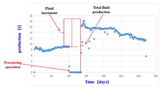
Figure 1.
Interpretation diagram illustrating total fluid production and incremental fluid production.
Table 1 shows that this difference resulted in the fluid increment per hour within 30 days after fracturing. After applying the four hierarchical allocation methods, these two target variables were expanded into 12 different production parameters, providing comprehensive and precise quantitative indicators for the subsequent model development.

Table 1.
Names of the 12 Production Parameters.
3.2. Data Preprocessing
To ensure accurate and comprehensive detection of outliers, this study employed a combination of three methods: the three-sigma rule, the median absolute deviation method, and the density-based spatial clustering of applications with noise algorithm. The three-sigma rule identifies outliers based on deviations from the mean under the assumption of a normal distribution; median absolute deviation improves robustness against skewed distributions by using the median as a central measure; and density-based spatial clustering of applications with noise detects local anomalies based on data density, capturing patterns that deviate from the general distribution. Outliers identified by all three methods were uniformly treated as missing values. These missing values were then imputed using the KNN, which estimates unknown entries by calculating feature similarity and referencing the values of the nearest neighbors. This approach preserves the internal correlation and distribution characteristics of the dataset. After preprocessing, a complete, continuous dataset was obtained, providing a high-quality foundation for subsequent feature selection and model construction.
3.3. Analysis of Dominant Influencing Factors
Following data cleansing and target variable selection, the next step was to analyze internal relationships among variables to improve model performance and predictive accuracy. This step aimed to identify representative features with strong correlations to the target variables, serving as a basis for effective feature selection and variable optimization during model development.
Pearson correlation analysis was conducted on the finalized dataset, including 13 geological parameters and 44 engineering parameters. The Pearson correlation coefficient quantifies the degree of linear relationship between two continuous variables by calculating the ratio of their covariance to the product of their standard deviations. Its value ranges from −1 to 1: values closer to 1 indicate a strong positive linear correlation, values closer to −1 reflect a strong negative linear correlation, and values near 0 imply no linear relationship.
To visualize these relationships, Pearson correlation coefficients were calculated for all pairs of fracturing-related parameters, resulting in a comprehensive correlation matrix. This matrix was then used to generate a heatmap to intuitively illustrate the correlation structure. Figure 2 shows the total liquid production volume over 30 days with a weighted distribution of permeability and thickness as the target variable. The heat map reflects the correlation degree through color gradients. Areas close to red indicate a positive correlation degree with a coefficient close to +1, while areas close to blue indicate a negative correlation degree with a coefficient close to −1. This visualization clearly reveals the strength and direction of the linear correlation between the input parameters.
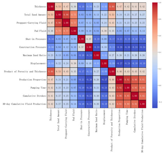
Figure 2.
Pearson Correlation Heatmap Analysis.
Based on the above analysis, the study first calculated the correlation coefficients between each input feature and the target production metrics and screened out candidate parameters with strong correlations. To mitigate the impact of multicollinearity on model stability, the variance inflation factor (VIF) method was further applied to evaluate the candidate parameters, setting the VIF threshold at <10 and eliminating redundant features with severe multicollinearity whose VIF values exceed this threshold. Ultimately, twelve parameters were selected as the dominant influencing factors for production, including strokes per hour, pumping time over the 30-day production period, ΦH, formation thickness, total proppant volume, maximum sand ratio, proppant-laden fluid volume, treatment pressure, injection rate, shut-in pressure, pre-pad fluid volume, and production contribution ratio. For the term “ΦH”, “Φ” denotes porosity and “H” denotes formation thickness; thus, “ΦH” represents the product of porosity and formation thickness.
3.4. Model Selection
Production forecasting in this study is treated as a typical regression problem in machine learning, where the objective is to model the functional relationship between multiple fracturing parameters and a single production outcome. The goal is to use this relationship to predict post-fracturing productivity.
Given the multidimensional, nonlinear, collinear, and noisy nature of fracturing datasets, and the requirements of regression tasks for model interpretability, generalization, robustness, and capacity to capture complex patterns, this study performed a systematic evaluation of various machine learning models and their suitability for the problem. Among linear models, ridge regression and lasso were selected for their ability to alleviate multicollinearity through regularization, Huber regression for its robustness to noise, PLS for its suitability in high-dimensional data through latent variable extraction, and standard linear regression as a baseline for linear fitting. Among nonlinear models, KNN captures local nonlinear patterns based on similarity, SVR maps complex relationships through kernel functions, and decision tree uses recursive partitioning for intuitive nonlinear modeling. Ensemble models include random forest, which improves generalization via model aggregation, and XGBoost, LGBM, and CatBoost—three gradient boosting algorithms that leverage deep pattern mining, with respective advantages in handling missing values, training efficiency, and categorical feature encoding. Based on this evaluation, twelve models were selected from three categories: KNN, linear regression, ridge regression, lasso regression, decision tree, SVR, Huber regression, XGBoost, random forest, PLS, LGBM, and CatBoost. These models encompass diverse algorithmic structures capable of adapting to the complex characteristics of fracturing data and provide a comprehensive basis for model comparison and optimal selection.
3.5. Model Training
To support production forecasting model training at multiple spatial scales, this study constructed seven datasets incorporating twelve distinct production parameters. The data preparation and partitioning process is outlined as follows:
The twelve production parameters were developed based on detailed disaggregation of multilayer commingled well production and quantification of fracturing effectiveness. Three core target variables were first defined:
- (1)
- The 30-day total fluid production after fracturing
- (2)
- The 30-day incremental fluid production, which is defined as the difference in total fluid production before and after fracturing
- (3)
- The hourly fluid increment, calculated by normalizing the pre- and post-fracturing 30-day total fluid production to account for differences in production duration.
To address the multilayer nature of the commingled wells, each of the three core parameters was further allocated to individual layers using four geological proportion-based splitting methods:
- (1)
- Layer thickness ratio,
- (2)
- Porosity–thickness product ratio
- (3)
- Permeability–thickness product ratio
- (4)
- Porosity–permeability–thickness combined product ratio.
Applying these four methods to the three target variables yielded a total of twelve production parameters for use in model development.
Based on reservoir characteristics across different blocks and formations, twelve key production parameters were systematically categorized into seven specialized datasets:
- (1)
- Regional composite dataset (436 wells, XL Port area)
- (2)
- Block-specific dataset (330 wells, Y63 block)
- (3)
- Block-specific dataset (106 wells, XL10 block)
- (4)
- Formation-specific dataset (79 wells, ES2 formation, Y63 block)
- (5)
- Formation-specific dataset (188 wells, ES3 formation, Y63 block)
- (6)
- Formation-specific dataset (22 wells, ES2 formation, XL10 block)
- (7)
- Formation-specific dataset (65 wells, ES3 formation, XL10 block)
The ES1 interval was not modeled separately due to insufficient data. All seven datasets consistently include the twelve previously defined production parameters, thereby covering different spatial scales—regional, block-level, and interval-level—across the study area. The use of a standardized parameter system ensures the comparability of data across these varying scales.
During the model training phase, to scientifically evaluate model performance, we conducted systematic optimization of the validation strategy based on the sample characteristics of each dataset: first, we tested different training-test set splitting ratios such as 7:3 and 9:1 and introduced k = 5 and k = 10 fold cross-validation for comparative analysis. The results showed that the 8:2 random splitting ratio achieved an optimal balance between ensuring the sufficiency of training samples and the representativeness of the test set. Its evaluation results were highly consistent with those of cross-validation, with a repeated deviation of less than 3%, which could effectively support the evaluation conclusions regarding the model’s fitting ability and generalization ability. Therefore, this ratio was ultimately adopted to divide each dataset into a training set and a test set, where the training set was used for model training and the test set was reserved for performance evaluation. In future research, we will further incorporate statistical methods such as confidence interval calculation and multiple comparison correction to enhance the rigor of result analysis.
To enhance the predictive performance of all algorithms and ensure the scientific soundness of parameter configurations, this study employed grid search for hyperparameter optimization of all models under comparison. The coefficient of determination (R2) was set as the optimization objective. By exhaustively searching all combinations within the parameter grid, this method identified the parameter configuration that maximized model performance. An R2 value closer to 1 indicates stronger explanatory power of the model for capturing production dynamic trends and lower prediction error. Regarding the selection of optimization methods, we simultaneously tested strategies such as Bayesian search. Comparative analysis revealed that grid search achieved more comprehensive parameter coverage, and the corresponding model exhibited superior performance with a repeated fluctuation of less than 3%, which could meet the accuracy requirements of this study.
Test results from the critical region dataset revealed performance variation among different production allocation methods. Specifically, using the permeability–thickness product ratio for allocating total fluid production yielded the highest prediction accuracy, while allocating incremental fluid production based on the porosity–permeability–thickness product ratio delivered the best results. To maintain a focused and targeted discussion in the subsequent analysis, only the models corresponding to these two best-performing allocation methods are further examined.
3.5.1. Overall Model Performance in the Critical Region
The model training results for the overall dataset from the critical region revealed notable differences in prediction accuracy across production parameters. As illustrated in Figure 3, Figure 4 and Figure 5, yellow bars represent R2 scores on the training set, while blue bars indicate performance on the testing set. The highest testing accuracy reached 73% for total fluid production, 71% for hourly fluid production, and 60% for incremental fluid production.
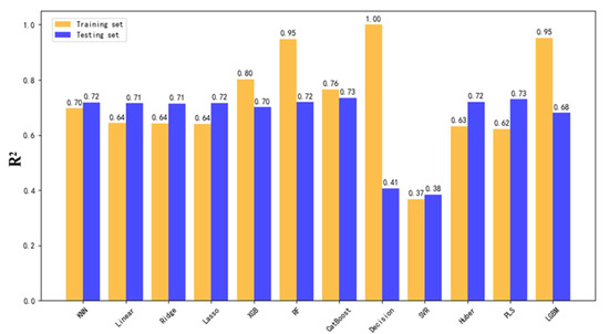
Figure 3.
Comparison of R2 Scores for Total Fluid Production Prediction Using 12 Models in the Overall Dataset.
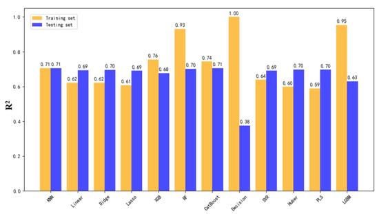
Figure 4.
Comparison of R2 Scores for Hourly Fluid Production Prediction Using 12 Models in the Overall Dataset.
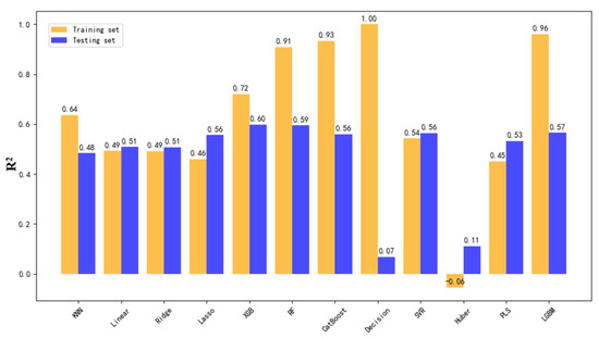
Figure 5.
Comparison of R2 Scores for Incremental Fluid Production Prediction Using 12 Models in the Overall Dataset.
To further investigate the prediction error of incremental fluid production, Figure 6 compares the test set prediction errors of the twelve models trained on the overall dataset. The performance is evaluated using both mean absolute error (MAE) and mean squared error (MSE), providing additional validation of model accuracy.
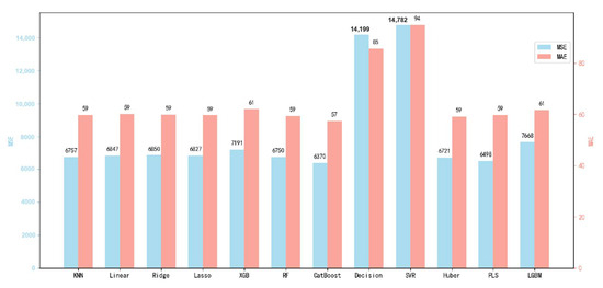
Figure 6.
Test set prediction error comparison for total fluid production using twelve models trained on the overall dataset.
Figure 7 and Figure 8 comparatively illustrate the model performance on the training and testing datasets, respectively, presenting a comprehensive evaluation of all twelve machine learning models. The visualizations incorporate three key performance metrics—mean absolute error, mean squared error, and the coefficient of determination—along with corresponding predicted-actual value scatter plots. In the scatter plots, the spatial distribution of data points relative to the diagonal reference line directly reflects prediction accuracy, with tighter clustering along the diagonal indicating superior model performance. These visualizations intuitively demonstrate the degree of alignment between model predictions and actual values, not only validating the R2 scores reported earlier but also providing a more comprehensive perspective for model performance evaluation.
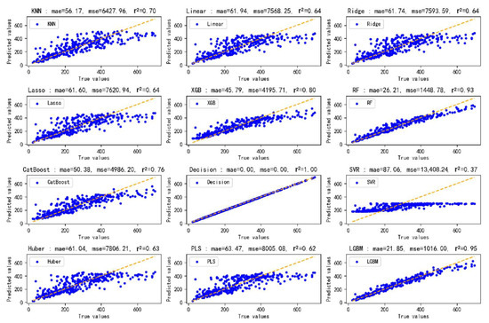
Figure 7.
Predicted vs. actual values on the training set for twelve models.
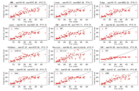
Figure 8.
Predicted vs. actual values on the test set for twelve models.
To further enhance the comprehensiveness and professional adaptability of the evaluation system, future studies will introduce more diverse performance evaluation metrics, including mean absolute percentage error (MAPE), root mean squared logarithmic error (RMSLE), as well as specialized evaluation metrics unique to the petroleum engineering field. This will enable more accurate and engineering-practice-aligned quantitative analysis of model prediction performance.
Figure 9 provides a direct performance comparison between the highest-performing CatBoost model and the lowest-performing SVR model. The proximity between the red dashed line and the green polyline in the visualization serves as a clear indicator of model training effectiveness. A visual examination reveals significantly superior fitting performance between these trend lines for the CatBoost model when compared to the SVR model. This comparative analysis not only demonstrates the distinct advantages of high-performance models but also highlights the inherent limitations of underperforming ones, thereby offering valuable guidance for subsequent model selection processes.
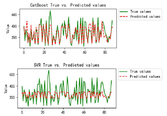
Figure 9.
Comparison between the best- and worst-performing models.
It is important to note that the figures above cover the major performance dimensions for the overall dataset. To avoid redundancy, similar visualizations will not be repeated in the analysis of other blocks or formations. Instead, only key results and conclusions will be summarized in text.
Further analysis reveals substantial geological differences between the Y63 and XL10 blocks, including reservoir physical properties and sedimentary facies. When the data from both blocks are merged for training, models struggle to generalize across these heterogeneous geological–engineering response patterns, resulting in limited predictive accuracy. This finding supports the strategy of modeling each block independently to better accommodate geological variability and enhance model generalization.
3.5.2. Overall Model Performance in the Y63 Block
Inspired by findings from the dataset, the Y63 block was modeled independently, resulting in a significant improvement in predictive performance. As shown in Figure 10, Figure 11 and Figure 12, the highest test set R2 scores reached 83% for hourly fluid production, 81% for total fluid production, and 73% for incremental fluid production.
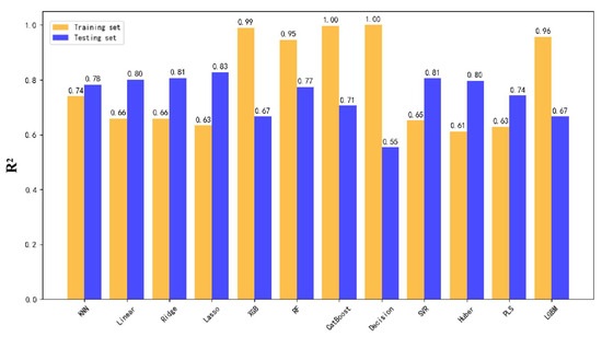
Figure 10.
R2 score comparison for hourly fluid production using twelve models trained on the Y63 block.
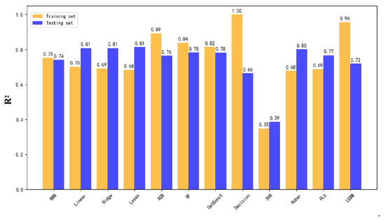
Figure 11.
R2 score comparison for total fluid production using twelve models trained on the Y63 block.
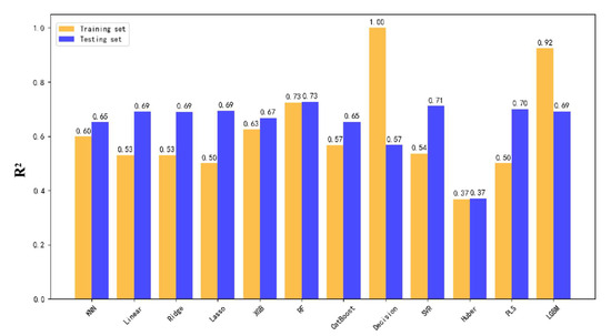
Figure 12.
R2 score comparison for incremental fluid production using twelve models trained on the Y63 block.
Compared to the results from the combined dataset, prediction accuracy improved by 8% to 13%, with the most significant gains observed in incremental fluid production. This validates the effectiveness of block-specific modeling, where models tailored to the high-porosity, high-permeability reservoirs and fluid-loss behaviors unique to the Y63 block can more accurately capture productivity trends.
3.5.3. Layer-Specific Modeling in the Y63 Block
Layer-level modeling was conducted for the ES2 and ES3 intervals of the Y63 block, further improving prediction accuracy:
ES2 interval: The models achieved the highest accuracy across all parameters. As shown in Figure 13, the best test set R2 scores were 90% for hourly fluid production, 88% for incremental fluid production, and 81% for total fluid production, representing a 7% to 15% improvement over the full-block model.
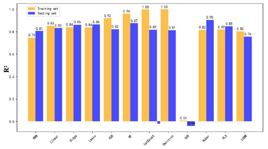
Figure 13.
R2 score comparison for total fluid production using twelve models trained on the Y63 ES2 interval.
The superior performance is attributed to the availability of 79 well samples, which adequately captured the geological characteristics and engineering parameters, enabling accurate modeling of layer-specific productivity patterns.
ES3 interval: While slightly lower than ES2, performance remained strong. Test set R2 scores reached 85% for total fluid production, 78% for hourly fluid production, and 72% for incremental fluid production. The 4% improvement in total fluid production accuracy compared to full-block modeling highlights the impact of interlayer geological heterogeneity on model performance.
These results confirm that accounting for geological variability through layer-specific modeling helps reduce interlayer interference and enhances the model’s ability to quantify the productivity of target intervals.
3.5.4. Overall Model Performance in the XL10 Block
In contrast to the Y63 block, the XL10 block models showed limited performance. The highest test set R2 scores reached only 75% for total fluid production, 74% for hourly fluid production, and 49% for incremental fluid production. The data from 106 wells is a relatively small training dataset, which is insufficient to fully capture the effects of reservoir heterogeneity and spatial variations in fracturing parameters. This hindered the model’s ability to learn the complex nonlinear mapping between geological–engineering inputs and production outputs.
3.5.5. Layer-Specific Modeling in the XL10 Block
Layer-specific models for the ES2 and ES3 intervals in the XL10 block further confirmed the limitations imposed by small datasets:
ES2 interval: With only 22 wells, model performance was low. Test set R2 scores were 48% for hourly fluid production, 51% for total fluid production, and 52% for incremental fluid production. The lack of data prevented the model from capturing thin-layer development and fracturing fluid-loss dynamics specific to this interval.
ES3 interval: Although the dataset of 65 wells is slightly larger than the ES2 interval, the model accuracy is still limited. The best test set R2 scores were 49% for hourly fluid production, 62% for total fluid production, and 67% for incremental fluid production. The strong reservoir heterogeneity and incomplete coverage of engineering variations contributed to these limitations.
To address the issue of uncertainty in small-sample data, future studies will further introduce resampling methods to quantify such uncertainty. Additionally, learning curve analysis will be employed to identify the core reasons for limited model performance, thereby refining the validation logic.
4. Discussion
The dataset used in this study is relatively small and exhibits uneven distribution across blocks and intervals. The Y63 block contains a relatively sufficient dataset of 339 well instances, achieving model accuracy ranging from 72% to 90%. In contrast, the XL10 block has only 106 well instances, resulting in model accuracy between 48% and 75%. This small-sample issue exacerbates risks of overfitting or underfitting, weakens the model’s generalization capability, and leads to suboptimal prediction accuracy. Furthermore, preprocessing steps—such as outlier detection and missing value imputation—applied to limited datasets with potential non-stationary distributions may introduce unintended biases. Future efforts should prioritize collecting additional well data for data-scarce blocks, investigating machine learning algorithms tailored for small-sample scenarios, and employing data augmentation techniques to enhance sample diversity and improve prediction accuracy.
The current model exhibits limited transferability beyond specific blocks within the Huabei Oilfield due to its heavy reliance on localized historical data. Despite acknowledging intra-regional variations, the model training inadequately incorporates universal geological characteristics spanning different regions or heterogeneous reservoir types. Future research must enhance model generalization by employing transfer learning techniques, integrating data from source blocks to support target block training. This should be coupled with the inclusion of broader geological context data, such as lithology and tectonic settings. Rigorous validation of the model’s adaptability across diverse subsurface conditions is essential to achieve this goal.
The feature selection and model optimization methodologies employed in this study present limitations. The current feature selection strategy, focusing predominantly on linear relationships and multicollinearity, risks neglecting critical nonlinear interactions between factors like fracturing fluid performance or reservoir stress and total fluid production. This oversight compromises the model’s interpretability and predictive capability. Regarding model optimization, while twelve algorithms were evaluated and grid search was implemented for hyperparameter tuning, grid search suffers from inefficiency in high-dimensional parameter spaces and the potential to miss global optima. Subsequent studies should prioritize feature importance-based screening methods capable of capturing nonlinear correlations. Furthermore, advanced hyperparameter optimization algorithms, for instance Bayesian optimization or genetic algorithms, should replace or supplement grid search to improve model efficiency and predictive performance.
5. Conclusions
This study developed a post-fracturing productivity prediction model to address commingled production challenges in multilayer reservoirs, leveraging data from 436 wells in a key block of the Huabei Oilfield. Twelve machine learning algorithms were employed to overcome limitations of conventional methods. Systematic collection and cleaning of raw logging, engineering, and production data enabled in-depth analysis of key parameters governing fracturing outcomes. Through advanced production allocation methods and targeted modeling strategies including block-specific and formation-specific approaches, significant performance variations were identified across blocks and formations. These disparities primarily stem from four factors: data volume, geological heterogeneity between blocks, formation characteristics, and applicability of target parameters.
This study demonstrates the significant influence of data volume and geological heterogeneity on production forecasting accuracy. A comparative analysis between the data-sufficient Y63 block and data-limited XL10 block reveals that prediction performance strongly depends on data availability, with Y63 achieving substantially higher accuracy. The results show that block-specific modeling outperforms mixed-block approaches by 8–13% in terms of prediction accuracy, underscoring the importance of considering geological variations in model development. Further refinement through reservoir-layer-specific modeling yields even better performance, as evidenced by the 90% prediction accuracy achieved for the ES2 formation in the Y63 block. Moreover, cumulative production data proves to be a more reliable predictor than incremental production data, with this finding being particularly prominent in the study area. These insights provide valuable guidance for production forecasting in similar oilfield reservoirs.
In summary, this model provides an effective tool for post-fracturing productivity forecasting while revealing fundamental differences in productivity patterns across blocks and formations. These findings offer critical insights for optimizing development plans and predicting productivity in new wells within the study area.
Author Contributions
Conceptualization, R.Z.; Methodology, N.L.; Software, F.Q.; Validation, C.L.; Formal analysis, X.W.; Resources, G.L. (Guohua Liu); Writing—original draft, F.L.; Visualization, S.X.; Supervision, G.L. (Gensheng Li); Project administration, Q.L. All authors have read and agreed to the published version of the manuscript.
Funding
This research was funded by the National Natural Science Foundation of China (grant number 52320105002 and 52374017), and PetroChina Huabei Oilfield Company (grant number HBYT-YQGYY-2024-JS-28).
Data Availability Statement
The data presented in this study are available on request from the corresponding author due to privacy restrictions from the company.
Conflicts of Interest
Authors Ruibin Zhu, Ning Li, Guohua Liu, Fengjiao Qu, Changjun Long, Xin Wang and Shuzhi Xiu were employed by Research Institute of Oil and Gas Technology, PetroChina Huabei Oilfield Company. The remaining authors declare that the research was conducted in the absence of any commercial or financial relationships that could be construed as a potential conflict of interest. The authors declare that this study received funding from the PetroChina Huabei Oilfield Company. The funder was not involved in the study design, collection, analysis, interpretation of data, the writing of this article, or the decision to submit it for publication.
References
- Li, H.; Luo, P.; Bai, Y. Summary for Machine Learning Algorithms and Their Applications in Drilling Engineering. Xinjiang Oil Gas 2022, 18, 13. [Google Scholar] [CrossRef]
- Davoodi, S.; Thanh, H.V.; Wood, D.A.; Mehrad, M.; Muravyov, S.V.; Rukavishnikov, V.S. Carbon dioxide storage and cumulative oil production predictions in unconventional reservoirs applying optimized machine-learning models. Pet. Sci. 2025, 22, 296–323. [Google Scholar] [CrossRef]
- Dai, Q.-Y.; Zhang, L.-M.; Zhang, K.; Hao, H.; Chen, G.-D.; Yan, X.; Liu, P.-Y.; Zhang, B.-B.; Wang, C.-Y. Integrated optimization of reservoir production and layer configurations using relational and regression machine learning models. Pet. Sci. 2025. [Google Scholar] [CrossRef]
- Liu, C.; Liu, P.; Wang, Q.; Zhang, L.; Huang, Z.; Xu, Y.; Jiang, S.; Zhang, L.; Cao, C. Stratified allocation method for water injection based on machine learning: A case study of the Bohai A oil and gas field. Nat. Gas Ind. B 2025, 12, 207–218. [Google Scholar] [CrossRef]
- Xiao, C.; Zhang, S.; Ma, X.; Zhou, T.; Li, X. Surrogate-assisted hydraulic fracture optimization workflow with applications for shale gas reservoir development: A comparative study of machine learning models. Nat. Gas Ind. B 2022, 9, 219–231. [Google Scholar] [CrossRef]
- Jia, J.; Li, D.; Wang, L.; Fan, Q. Novel Transformer-based deep neural network for the prediction of post-refracturing production from oil wells. Adv. Geo-Energy Res. 2024, 13, 119–131. [Google Scholar] [CrossRef]
- Chakra, N.C.; Song, K.Y.; Gupta, M.M.; Saraf, D.N. An innovative neural forecast of cumulative oil production from a petroleum reservoir employing higher-order neural networks (HONNs). J. Pet. Sci. Eng. 2013, 106, 18–33. [Google Scholar] [CrossRef]
- Sheremetov, L.; Cosultchi, A.; Martínez-Muñoz, J.; Gonzalez-Sánchez, A.; Jiménez-Aquino, M. Data-driven forecasting of naturally fractured reservoirs based on nonlinear autoregressive neural networks with exogenous input. J. Pet. Sci. Eng. 2014, 123, 106–119. [Google Scholar] [CrossRef]
- Amr, S.; El Ashhab, H.; El-Saban, M.; Schietinger, P.; Caile, C.; Kaheel, A.; Rodriguez, L. A large-scale study for a multi-basin machine learning model predicting horizontal well production. In Proceedings of the SPE Annual Technical Conference and Exhibition, Dallas, TX, USA, 24–26 September 2018; SPE: Bellingham, WA, USA, 2018. [Google Scholar]
- Pankaj, P.; Shukla, P.; Wang, W.K. Hydraulic Fracture Calibration for Unconventional Reservoirs: A New Methodology for Predictive Modelling. In Proceedings of the International Petroleum Technology Conference, Beijing, China, 26–28 March 2019. [Google Scholar]
- Cao, Q.; Banerjee, R.; Gupta, S.; Li, J.; Zhou, W.; Jeyachandra, B. Data Driven Production Forecasting Using Machine Learning. In Proceedings of the SPE Argentina Exploration and Production of Unconventional Resources Symposium, Buenos Aires, Argentina, 1–3 June 2016. [Google Scholar]
- Lolon, E.; Hamidieh, K.; Weijers, L.; Mayerhofer, M.; Melcher, H.; Oduba, O. Evaluating the Relationship Between Well Parameters and Production Using Multivariate Statistical Models: A Middle Bakken and Three Forks Case History. In Proceedings of the SPE Hydraulic Fracturing Technology Conference, The Woodlands, TX, USA, 9–11 February 2016. [Google Scholar]
- Sagheer, A.E.; Kotb, M. Time series forecasting of petroleum production using deep LSTM recurrent networks. Neurocomputing 2019, 323, 203–213. [Google Scholar] [CrossRef]
- Abdrakhmanov, I.R.; Kanin, E.A.; Boronin, S.A.; Burnaev, E.V.; Osiptsov, A.A. Development of Deep Transformer-Based Models for Long-Term Prediction of Transient Production of Oil Wells. In Proceedings of the SPE Russian Petroleum Technology Conference, Online, 12–15 October 2021. [Google Scholar]
- Dong, P.; Liao, X. A Deep-Learning-Based Approach for Production Forecast and Reservoir Evaluation for Shale Gas Wells with Complex Fracture Networks. In Proceedings of the SPE EuropEC—Europe Energy Conference Featured at the 83rd EAGE Annual Conference & Exhibition, Madrid, Spain, 6–9 June 2022. [Google Scholar]
- Shahkarami, A.; Ayers, K.; Wang, G.; Ayers, A. Application of Machine Learning Algorithms for Optimizing Future Production in Marcellus Shale, Case Study of Southwestern Pennsylvania. In Proceedings of the SPE/AAPG Eastern Regional Meeting, Pittsburgh, PA, USA, 7–11 October 2018. [Google Scholar]
- Pranesh, V.; Thamizhmani, V.; Ravikumar, S.; Padakandla, S. Multiple linear regression theory based performance optimization of Bakken and Eagle Ford shale oil reservoirs. Int. J. Eng. Res. Appl. 2018, 8, 66–88. [Google Scholar]
- Luo, S.; Ding, C.; Cheng, H.; Zhang, B.; Zhao, Y.; Liu, L. Estimated ultimate recovery prediction of fractured horizontal wells in tight oil reservoirs based on deep neural networks. Adv. Geo-Energy Res. 2022, 6, 111–122. [Google Scholar] [CrossRef]
- Alwated, B.; El-Amin, M.F. Enhanced oil recovery by nanoparticles flooding: From numerical modeling improvement to machine learning prediction. Adv. Geo-Energy Res. 2021, 5, 297–317. [Google Scholar] [CrossRef]
- Wu, C.; Wang, S.; Yuan, J.; Li, C.; Zhang, Q. A prediction model of specific productivity index using least square support vector machine method. Adv. Geo-Energy Res. 2020, 4, 460–467. [Google Scholar] [CrossRef]
- Zhao, W.; Wang, W.; Zheng, M.; Luo, D.; Xie, M.; Wu, Y. Comprehensive Correlation Analysis of Influencing Factors of Shale Gas Productivity Based on Adaptive Lasso Regression. In Proceedings of the Abu Dhabi International Petroleum Exhibition and Conference, Abu Dhabi, United Arab Emirates, 2–5 October 2023; SPE: Bellingham, WA, USA, 2023; p. D022S183R003. [Google Scholar]
- Noshi, C.I.; Eissa, M.R.; Abdalla, R.M. An intelligent data driven approach for production prediction. In Proceedings of the Offshore Technology Conference, Houston, TX, USA, 6–9 May 2019; OTC: Houston, TX, USA, 2019; p. D041S048R007. [Google Scholar]
- Ma, H.; Zhao, W.; Zhao, Y.; He, Y. A Data-Driven Oil Production Prediction Method Based on the Gradient Boosting Decision Tree Regression. Comput. Model. Eng. Sci. 2023, 134, 1773–1790. [Google Scholar] [CrossRef]
- Sharma, A.; Gupta, I.; Phi, T.; Ashesh, S.; Kumar, R.; Borgogno, F.G. Utilizing machine learning to improve reserves estimation and production forecasting accuracy. In Proceedings of the Latin America Unconventional Resources Technology Conference, Buenos Aires, Argentina, 4–6 December 2023; Unconventional Resources Technology Conference (URTeC): Houston, TX, USA, 2024; pp. 145–164. [Google Scholar]
- Xue, L.; Liu, Y.; Xiong, Y.; Liu, Y.; Cui, X.; Lei, G. A data-driven shale gas production forecasting method based on the multi-objective random forest regression. J. Pet. Sci. Eng. 2021, 196, 107801. [Google Scholar] [CrossRef]
- Chen, T.; Guestrin, C. Xgboost: A scalable tree boosting system. In Proceedings of the 22nd ACM SIGKDD International Conference on Knowledge Discovery and Data Mining, San Francisco, CA, USA, 13–17 August 2016; pp. 785–794. [Google Scholar]
- Liu, W.; Chen, Z.; Hu, Y.; Xu, L. A systematic machine learning method for reservoir identification and production prediction. Pet. Sci. 2023, 20, 295–308. [Google Scholar] [CrossRef]
- Tan, C.; Yang, J.; Cui, M.; Wu, H.; Wang, C.; Deng, H.; Song, W.; Xiong, H. Fracturing productivity prediction model and optimization of the operation parameters of shale gas well based on machine learning. Lithosphere 2021, 2021, 2884679. [Google Scholar] [CrossRef]
- Omotosho, T.J. Oil Production Prediction Using Time Series Forecasting and Machine Learning Techniques. In Proceedings of the SPE Nigeria Annual International Conference and Exhibition, Lagos, Nigeria, 5–7 August 2024; SPE: Bellingham, WA, USA, 2024; p. D032S028R006. [Google Scholar]
- Tranmer, M.; Elliot, M. Multiple linear regression. Cathie Marsh Cent. Census Surv. Res. (CCSR) 2008, 5, 1–5. [Google Scholar]
- Hoerl, A.E.; Kennard, R.W. Ridge regression: Biased estimation for nonorthogonal problems. Technometrics 1970, 12, 55–67. [Google Scholar] [CrossRef]
- Tibshirani, R. Regression shrinkage and selection via the lasso. J. R. Stat. Soc. Ser. B Stat. Methodol. 1996, 58, 267–288. [Google Scholar] [CrossRef]
- Wold, S.; Ruhe, A.; Wold, H.; Dunn, W.J., III. The collinearity problem in linear regression. The partial least squares (PLS) approach to generalized inverses. SIAM J. Sci. Stat. Comput. 1984, 5, 735–743. [Google Scholar] [CrossRef]
- Cortes, C.; Vapnik, V. Support-vector networks. Mach. Learn. 1995, 20, 273–297. [Google Scholar] [CrossRef]
- Huber, P.J. Robust estimation of a location parameter. In Breakthroughs in Statistics: Methodology and Distribution; Springer: New York, NY, USA, 1992; pp. 492–518. [Google Scholar]
- Cover, T.; Hart, P. Nearest neighbor pattern classification. IEEE Trans. Inf. Theory 1967, 13, 21–27. [Google Scholar] [CrossRef]
- Breiman, L.; Friedman, J.; Olshen, R.A.; Stone, C.J. Classification and Regression Trees; Chapman and Hall/CRC: Boca Raton, FL, USA, 2017. [Google Scholar]
- Breiman, L. Random forests. Mach. Learn. 2001, 45, 5–32. [Google Scholar] [CrossRef]
- Ke, G.; Meng, Q.; Finley, T.; Wang, T.; Chen, W.; Ma, W.; Ye, Q.; Liu, T.Y. Lightgbm: A highly efficient gradient boosting decision tree. In Proceedings of the NIPS’17: 31st International Conference on Neural Information Processing Systems, Long Beach, CA, USA, 4–9 December 2017. [Google Scholar]
- Prokhorenkova, L.; Gusev, G.; Vorobev, A.; Dorogush, A.V.; Gulin, A. CatBoost: Unbiased boosting with categorical features. In Proceedings of the NIPS’18: 32nd International Conference on Neural Information Processing Systems, Montréal, QC, Canada, 3–8 December 2018. [Google Scholar]
Disclaimer/Publisher’s Note: The statements, opinions and data contained in all publications are solely those of the individual author(s) and contributor(s) and not of MDPI and/or the editor(s). MDPI and/or the editor(s) disclaim responsibility for any injury to people or property resulting from any ideas, methods, instructions or products referred to in the content. |
© 2025 by the authors. Licensee MDPI, Basel, Switzerland. This article is an open access article distributed under the terms and conditions of the Creative Commons Attribution (CC BY) license (https://creativecommons.org/licenses/by/4.0/).