Article

A Displacement Monitoring Model for High-Arch Dams Based on SHAP-Driven Ensemble Learning Optimized by the Gray Wolf Algorithm

1
Yellow River Engineering Consulting Co., Ltd., Zhengzhou 450003, China
2
College of Water Conservancy and Hydropower Engineering, Hohai University, Nanjing 210024, China
3
Key Laboratory of Water Management and Water Security for Yellow River Basin, Ministry of Water Resources (Under Construction), Zhengzhou 450003, China
4
The National Key Laboratory of Water Disaster Prevention, Hohai University, Nanjing 210024, China
5
Cooperative Innovation Center for Water Safety and Hydro Science, Hohai University, Nanjing 210024, China
*
Author to whom correspondence should be addressed.
Water 2025, 17(18), 2766; https://doi.org/10.3390/w17182766
Submission received: 13 August 2025 / Revised: 12 September 2025 / Accepted: 16 September 2025 / Published: 18 September 2025

Abstract

Displacement monitoring data is essential for assessing the structural safety of high-arch dams. Existing models, predominantly based on single-model architectures, often lack the ability to effectively integrate multiple algorithms, leading to limited predictive performance and poor interpretability. This study proposes an ensemble learning framework for dam displacement prediction, combining Hydraulic–Seasonal–Temporal model (HST), Random Forest (RF), and Bidirectional Gated Recurrent Unit (BiGRU) models as base learners. A stacking strategy is employed to enhance predictive accuracy, and the Grey Wolf Optimizer (GWO) is used for hyperparameter optimization. To improve model transparency, the Shapley Additive Explanations (SHAP) algorithm is applied for interpretability analysis. Extensive experiments demonstrate that the proposed ensemble model outperforms individual models, achieving a Root Mean Squared Error (RMSE) of 0.2241 and a Coefficient of Determination (R2) of 0.9993 on the test set. The SHAP analysis further elucidates the contribution of key variables, providing valuable insights into the displacement prediction process and offering a robust technical foundation for arch dam safety monitoring and early risk warning.

1. Introduction

As a critical dam type in hydraulic engineering, arch dams have delivered substantial economic and ecological benefits through their roles in power generation, flood control, and water resource management [1,2]. However, with the increasing height and scale of such structures, ensuring their operational safety has become a significant challenge. Among various monitoring indicators, deformation represents a direct manifestation of a dam’s structural behavior, making accurate deformation prediction essential for reliable safety assessment. Compared with conventional arch dams, high-arch dams exhibit more complex structural responses due to their increased geometric and mechanical complexity. Consequently, traditional displacement prediction models often fall short in meeting the high-precision monitoring requirements demanded by these large-scale infrastructures [3].
Among existing approaches, statistical models remain the most widely adopted for deformation monitoring due to their simplicity and interpretability. However, these models are inherently constrained by linear assumptions, making them inadequate for capturing the complex nonlinear coupling mechanisms between deformation fields and influencing factors, thereby limiting their predictive accuracy and generalization capability [4,5,6,7]. Finite element methods (FEM) [8,9,10,11], although capable of simulating dam deformation based on physical principles, are highly sensitive to material parameter uncertainties and prone to performance degradation under the influence of local data noise. In recent years, machine learning methods (such as Support Vector Machines (SVM) [12,13,14,15]) and deep learning technologies [16] (including Long Short-Term Memory (LSTM) [17,18] and Gated Recurrent Units (GRU) [19]) have been increasingly applied to dam deformation prediction. Numerous studies [2,20,21,22,23] have shown that these models exhibit significant advantages in simulating temporal features and capturing the delayed effects of environmental factors. Combining data mining methods like Dynamic Time Warping (DTW) [24] and Entropy [25] helps improve the model’s ability to handle misaligned or noisy data, further enhancing feature extraction. Specifically, architectures based on LSTM and GRU, as well as their variants BiLSTM [26] and BiGRU [27], have demonstrated exceptional performance. BiLSTM and BiGRU effectively capture temporal features through gating mechanisms while processing both forward and backward information, enabling them to better capture reverse dependencies in time series. Therefore, they excel at capturing long-term dependencies and complex temporal dynamics, making them particularly suitable for simulating the delayed effects of environmental factors in dam deformation prediction.
While the aforementioned methods have advanced dam displacement prediction from various perspectives, they commonly rely on single-model architectures, rendering them susceptible to inherent limitations of the respective modeling paradigms. Statistical models are constrained by strong prior assumptions; machine learning algorithms are prone to local minima; and deep learning approaches, despite their powerful representation capabilities, often lack interpretability and demand high computational resources. In response to these challenges, ensemble learning methods, by employing a variety of strategies, construct heterogeneous model fusion frameworks that effectively integrate the complementary strengths of linear and nonlinear models, as well as statistical and deep learning techniques, thereby improving prediction accuracy while enhancing model robustness. For instance, ref. [28] proposed a two-layer stacking ensemble that integrates XGBoost, Extra-Trees, and Support Vector Regression (SVR) as base learners, with Multiple Linear Regression (MLR) serving as the meta-learner, successfully leveraging the strengths of multiple models to improve prediction performance. Similarly, ref. [29] employed a Light Gradient Boosting Machine (LGBM)-based ensemble to predict dam displacement from denoised datasets, achieving superior predictive accuracy. Ref. [30] adopted Gaussian Process Regression (GPR) as a meta-learner to integrate MLR, RF, SVM, and deformation factor interpretation models, resulting in a robust and highly accurate predictive framework. Ref. [31] utilized the Soft Voting ensemble strategy to combine the results of three predictors (CatBoost Classifier (CBC), Random Forest Classifier (RFC), and Gradient Boost Classifiers (GBC)), achieving high-accuracy prediction for soil liquefaction. These studies demonstrate that different ensemble methods possess unique advantages in terms of model diversity and prediction accuracy.
Ensemble learning methods, by integrating diverse algorithms and factor-based models, have demonstrated strong potential in improving the accuracy and robustness of dam deformation prediction. However, the reliance on aggregated outputs from multiple sub-models often leads to a lack of transparency, posing challenges for interpretability. In the context of high arch dam safety monitoring, elucidating the causal relationships between influencing factors and predictive outcomes is essential for understanding deformation behavior and enabling mechanism-based safety assessments. To address this issue, an increasing number of studies have focused on enhancing the interpretability of predictive models. For example, ref. [32] employed the built-in feature importance mechanism of the XGBoost model to quantify the contribution of various factors to deformation prediction, thereby identifying dominant influencing variables across different temporal scales. Similarly, ref. [33] integrated the SHAP algorithm into their model to identify and interpret key features affecting seepage behavior predictions in embankment dams, achieving a mechanistic understanding of the seepage process. Despite these efforts, interpretability studies specifically targeting ensemble learning models in dam deformation prediction remain relatively limited, indicating a significant research gap in the field.
To address the aforementioned challenges, this study proposes an interpretable ensemble learning framework tailored for arch dam displacement prediction, which uniquely integrates traditional statistical models, machine learning algorithms, and deep learning architectures. The selection of base models—namely, the HST model from statistical approaches, BiGRU from deep learning, and RF from machine learning—was based on a comprehensive evaluation of predictive performance and pairwise Pearson correlation coefficients of model errors. This multi-model approach not only enhances model diversity but also mitigates ensemble bias that often arises from excessive homogeneity among base learners. The use of the Grey Wolf Optimization (GWO) algorithm for hyperparameter optimization further distinguishes this study, allowing for more efficient fine-tuning and improving model performance. To integrate the predictions from these selected base models, a stacking ensemble strategy was employed, which leverages the individual strengths of each model in capturing different aspects of the data distribution and feature interactions. This integration significantly enhances the overall prediction accuracy while maintaining a high level of interpretability. Furthermore, the SHAP algorithm was applied to quantify and rank the importance of all contributing factors, thereby ensuring the interpretability and transparency of the model, which is often a challenge in complex ensemble methods. By combining these approaches, this study not only improves predictive accuracy but also provides a mechanism-based understanding of the causal relationships influencing dam displacement, which is crucial for effective safety assessments. In the field of dam safety monitoring, similar studies that integrate multiple dam deformation prediction techniques and conduct interpretability analysis are rarely reported. This work contributes to advancing the field by combining these specific techniques within a unified framework, offering a novel approach to high-arch dam deformation prediction.
The structure of this paper is organized as follows: Section 2 presents the model methodology. Section 3 outlines the model architecture. Section 4 introduces the case study, details the design of comparative experiments, and verifies the effectiveness and interpretability of the proposed model through empirical analysis. Finally, Section 5 summarizes the main findings and offers perspectives for future research.

2. Methodology

Ensemble learning enhances model generalization by combining the predictive capabilities of multiple base learners. The ensemble approach adopted in this study employs a two-tiered architecture. The first layer consists of a set of heterogeneous base learners, each independently modeling the original dataset in parallel. The second layer integrates the preliminary predictions generated by the base models through an ensemble strategy, thereby achieving an optimized aggregation of the initial predictive outputs.

2.1. Base Learner Library

(1)
Base Learner 1: HST Model
The deformation of arch dams is primarily induced by three factors: reservoir water level, temperature variations, and time-dependent effects.
δ = δ H + δ T + δ θ
The water level factor is directly associated with fluctuations in the reservoir level. As the water level rises or falls, the corresponding change in hydrostatic pressure acting on the dam structure induces measurable deformation. In this study, the water level-induced deformation is represented by the following expression:
δ H = i = 0 3 a i H i
where a i denotes the regression coefficient corresponding to the hydrostatic pressure component, and H represents the upstream water level on the current observation day.
The temperature factor reflects the influence of ambient air temperature variations on the arch dam. Due to the arching effect of the dam structure, temperature changes induce thermal expansion and contraction of the concrete, resulting in periodic displacement behavior. In this study, the temperature-induced deformation is modeled using the following expression:
δ T = j = 1 2 b 1 j sin 2 π j t 365 + b 2 j cos 2 π j t 365
where b 1 j and b 2 j are the regression coefficients corresponding to the temperature-related components, and t denotes the cumulative number of days from the initial observation date to the current observation day.
The time-dependent factor captures the time-dependent characteristics of concrete materials, such as creep, that manifest during long-term service. Incorporating the time-effect factor into the displacement prediction model facilitates a more accurate representation of the dam’s long-term deformation behavior. In this study, the time-dependent deformation is described by the following expression:
δ θ = c 1 θ + c 2 ln θ
where θ = t 100 , t denotes the cumulative number of days from the initial observation date to the current observation day.
(2)
Base Learner 2: Random Forests
Random Forest [5,34,35] is a machine learning algorithm that constructs a predictive model by aggregating the outputs of multiple decision trees, aiming to enhance both accuracy and stability. Each decision tree within the forest is trained on a bootstrap sample, generated by sampling with replacement from the original dataset. The detailed workflow is illustrated in Figure 1. For regression tasks, the final prediction of the Random Forest model is obtained by calculating the mean of the outputs from all individual decision trees. The corresponding mathematical expression is as follows:
y = 1 n t r e e i = 1 n t r e e y i x
where y i x represents the predicted output corresponding to the input vector, and n t r e e denotes the total number of decision trees in the forest. The detailed implementation steps are shown in Figure 1.
(3)
Base Learner 3: Support Vector Machine
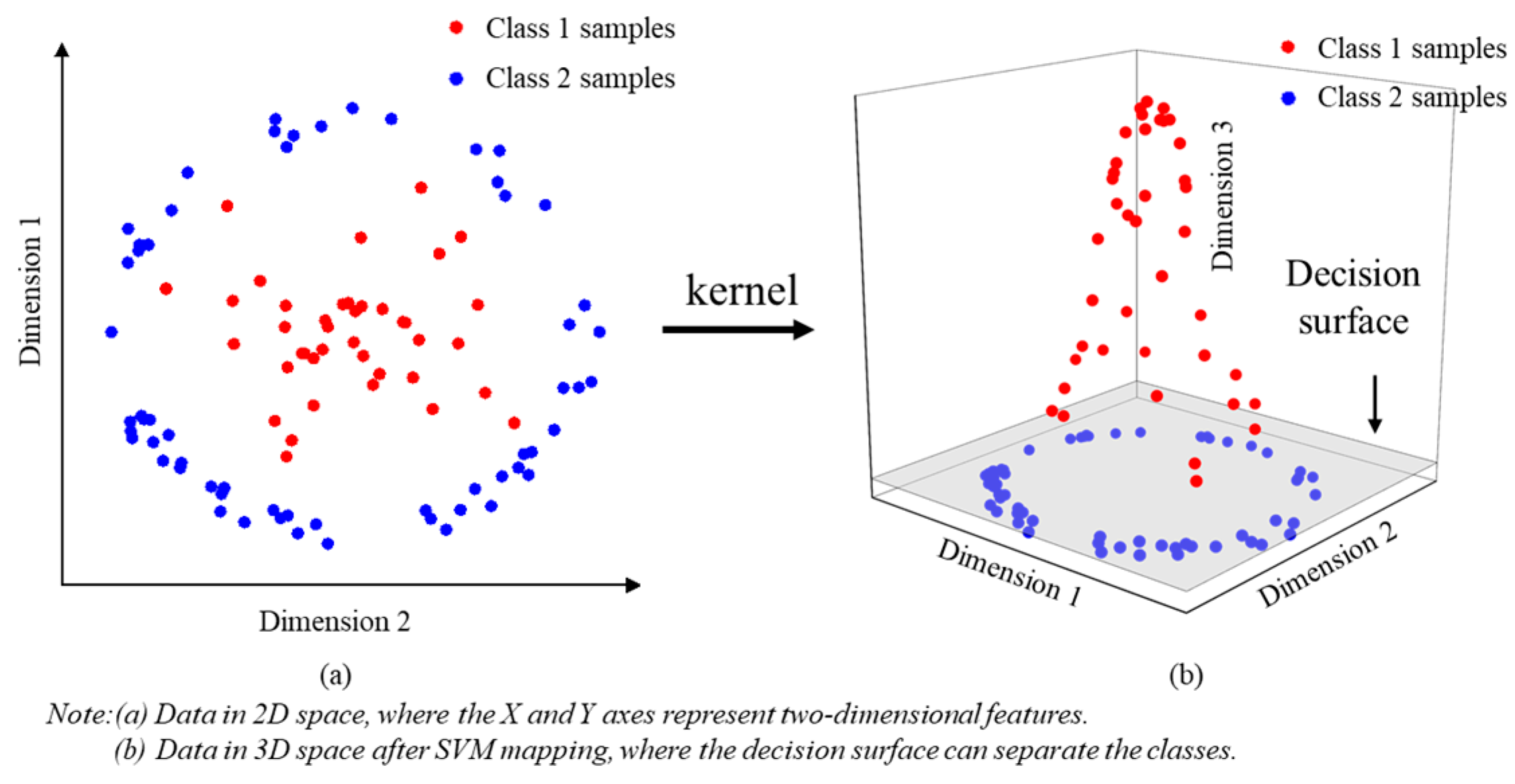
SVM is a supervised learning method grounded in statistical learning theory, well-suited for handling nonlinear time series prediction problems. In this study, the Radial Basis Function (RBF) kernel is employed to extract nonlinear features and complex patterns from the data, as illustrated in Figure 2.
The RBF kernel is defined as follows:
K x i , y i = exp γ x i y i 2
where γ > 0 is the kernel parameter that determines the strength of the similarity mapping between samples. The objective of SVM is to find the optimal function f x y within an acceptable error margin ε . The corresponding optimization objective is defined as follows:
min ω , b , ξ , ξ * 1 2 ω 2 + C i = 1 N ξ i + ξ i *
subject to the following constraints:
y i ω Φ x ω Φ x i + b ε + ξ b ε + ξ i ξ i , ξ i * 0
where ω is the weight vector, b is the bias term, ξ , ξ * are slack variables, C > 0 is the regularization parameter, and Φ ( x i ) is the mapping function to a high-dimensional feature space.
(4)
Base Learner 4: K-Nearest Neighbors(KNN) algorithm
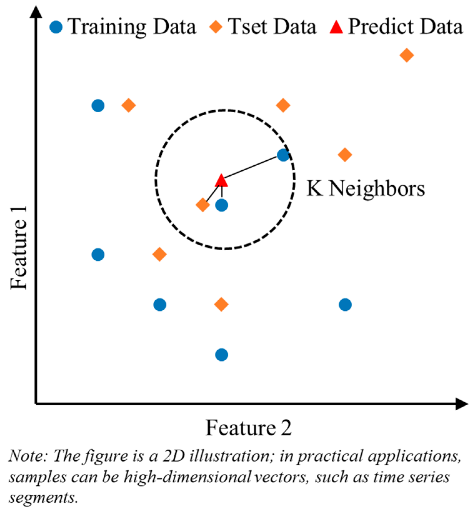
KNN algorithm [36] is a simple yet effective supervised learning method. Its core principle is to make predictions based on the attribute information of the K samples in the training set that are most similar to the target instance. The detailed process is illustrated in Figure 3.
In this study, the similarity between samples is measured using DTW. The corresponding calculation formula is as follows:
D T W ( X , Y ) = min ( i , j )   path   x i y j 2
where x i and y i represent the feature values of samples x and y in the i dimension, respectively, and n denotes the number of feature dimensions. In time series prediction tasks, a sample typically refers to a segment of time series data within a time window (or sliding window).
(5)
Base Learner 5: The Bidirectional Long Short-Term Memory network
The Bidirectional Long Short-Term Memory network (BiLSTM) [25] is an extension of the standard LSTM model, designed to enhance contextual modeling by incorporating both forward and backward temporal information. This bidirectional architecture improves the model’s ability to capture semantic dependencies in time series data, thereby increasing prediction accuracy. The core structure consists of two LSTM layers operating in opposite directions: one processes the sequence in forward order, while the other handles it in reverse. Their respective outputs are concatenated to form the final temporal feature representation. A schematic illustration is provided in Figure 4.
Taking the forward LSTM as an example, the specific network architecture is illustrated in Figure 5. The unit computation is as follows: Let the input sequence be denoted as x 1 , x 2 , x 3 , , x T , i t f represents the input gate, f t f denotes the forget gate, c t f is the self-update of the cell state, o t f corresponds to the output gate, and h t f is the final output. The structure of the backward LSTM is identical, except that the temporal order is reversed, as shown in the figure.
i t f = σ W i h t 1 , x t + b i f t f = σ W f h t 1 , x t + b f c t f = f t c t 1 + i t tan h W c h t 1 , x t + b c o t f = σ W x o x t + W h o h t 1 + W c o c t + b o h t f = o t tan h c t
The final output is obtained by concatenating the forward and backward hidden states.
h t = h t f , h t b
The output of the forward LSTM is denoted as h t f , while the output of the backward LSTM is denoted as h t b . After concatenation, the combined representation h t serves as the final output of the BiLSTM.
(6)
Base Learner 6: BiGRU
BiGRU [26] is a neural network model that extends the standard GRU by introducing a bidirectional architecture. It captures both forward and backward dependencies in a sequence, thereby enhancing the model’s ability to represent temporal dynamics. Compared with BiLSTM, BiGRU features a more compact structure, utilizing update and reset gates to control the flow of information and the updating of hidden states.
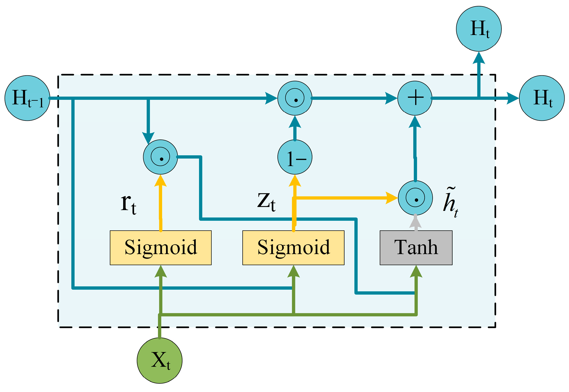
The computation of the forward GRU unit is as follows. A detailed schematic of the structure can be found in Figure 6.
z t f = σ W z x t + U z h t 1 + b z r t f = σ W r x t + U r h t 1 + b r h ~ t f = tan h W h x t + U h r t h t 1 + b h h t f = 1 z t h t 1 + z t h ~ t
In this context, z t serves as the update gate, controlling the fusion of new and old information, while r t acts as the reset gate, regulating the degree of historical information retention. h ~ t represents the candidate hidden state, which is a function of the current input and the previous hidden state after being modulated by the reset gate. The final hidden state h t is computed as the weighted sum of the previous hidden state and the candidate hidden state, with the weight determined by the update gate z t . The final output of the BiGRU, akin to that of the BiLSTM, is derived from the concatenation of the forward and backward GRU hidden layer outputs, with the specific formula corresponding to Equation (11).

2.2. Model Ensemble Methods

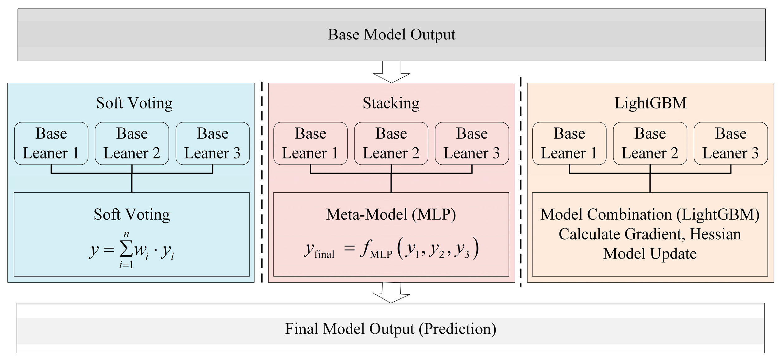
Traditional ensemble learning commonly employs strategies such as averaging and voting to combine the outputs of different base learners. While these methods can provide a reasonable approximation of model weighting, they often fail to capture the potential nonlinear interactions among the outputs of heterogeneous learners. To address the limitations of single-model approaches in modeling such complex relationships, this study explores three effective ensemble strategies: Soft Voting, Stacking based on a Multi-Layer Perceptron (MLP), and an integration method based on the LightGBM model. A schematic overview of these approaches is provided in Figure 7.
Weighted Averaging (Soft Voting): This method combines the predictions of multiple base models by performing a weighted average of their outputs. By assigning higher weights to more reliable models, it aims to optimize the final prediction outcome.
Stacking: Stacking is an ensemble strategy that takes the outputs of multiple base models as new input features and employs a meta-learner to generate the final prediction. In this study, a Multi-Layer Perceptron (MLP) is selected as the meta-learner. By learning the performance patterns of different base models across various samples, the meta-learner adaptively assigns weights, thereby enhancing prediction stability and generalization capability.
LightGBM-Based Integration: In this study, the LightGBM model, based on gradient boosting, is employed to learn and fuse the prediction outputs of multiple heterogeneous base models. Leveraging LightGBM’s superior nonlinear modeling capability and built-in feature importance evaluation mechanism, this approach effectively captures complex nonlinear interactions among base learner outputs, thereby improving the accuracy and robustness of the ensemble prediction. This method not only enhances the representational power of the integrated model but also increases the flexibility in aggregating information from diverse predictive sources.

2.3. GWO Optimization Algorithm

To enhance model diversity while further accelerating training and exploring the full potential of individual base learners, this study introduces the GWO algorithm [37] for hyperparameter optimization of base models. This optimization is essential for improving the prediction accuracy of these models, and GWO algorithm provides an effective solution by balancing exploration and exploitation during the optimization process. By leveraging GWO’s capability to explore a vast search space and fine-tune hyperparameters, the ensemble model’s performance is significantly enhanced. GWO minimizes the risk of overfitting and ensures that the optimized parameters yield the best performance across all base learners. This results in an ensemble model with high accuracy and robustness, capable of making more reliable predictions for dam displacement monitoring.
The GWO algorithm is a novel population-based metaheuristic optimization technique inspired by the social hierarchy and hunting behavior of grey wolves.By analyzing the hierarchical structure and predatory behavior of the wolf pack, wolves can be classified into four categories in descending rank: α , β , δ , ω . The α wolf serves as the leader of the pack, responsible for decision-making and other key behaviors. The β and δ wolves are capable of assuming leadership and decision-making roles should the α lose its position. The ω wolf plays a crucial role in maintaining internal balance within the pack.
The mathematical model for the encirclement is expressed as follows:
D w = C p × X w ( t ) X ( t ) X p = X w ( t ) A p × D w X ( t + 1 ) = p = 1 3 X p 3
In the equation, A p and C p are coefficients; t represents the current iteration number; D w denotes the distance between the gray wolf and the prey; X p indicates the position of the prey (optimal solution) in the t generation; and X ( t ) and X ( t + 1 ) represent the positions of the t and t + 1 generation gray wolves, respectively.
The values of A p and C p are influenced by a , and a dynamic search update strategy is employed. The calculation formula is as follows:
A = 2 a × r 1 a C = 2 r 2
r 1 and r 2 are two random vectors with values in the range [0, 1].
T represents the maximum number of iterations set for the algorithm. a is a parameter whose value decreases from 2 to 0, denoted as a i , where i indicates the current iteration. The value of a i varies within the interval [0, 2]. When a i is close to 2, it signifies that the gray wolves are gradually approaching the prey, prompting the pack to engage in an attack behavior, which corresponds to the exploitation phase of the algorithm. Conversely, when a i approaches 0, it indicates that the gray wolves are moving away from the prey, aiming to find a more suitable target, thereby encouraging the pack to perform a global search, which corresponds to the exploration phase of the algorithm.
a i = 2 2 × t T

2.4. Explainable Machine Learning Framework (SHAP)

The SHAP model [38] is used to interpret the predictions of machine learning models. Its core idea is to quantify the contribution of each input feature to the model’s output by computing its average marginal contribution across all possible combinations of feature subsets. Compared with other feature importance metrics, SHAP offers two key advantages: (1) it provides a unified framework for ranking feature importance, and (2) it satisfies the property of consistency when attributing contributions. The SHAP value for the i feature is computed as follows:
Φ i = S M { i } | S | ! ( | N | | S | 1 ) ! | N | ! ( ν ( S { i } ) ν ( S ) )
In the equation, N represents the set of all features, and S denotes the set that excludes the i influencing factor. | S | refers to the number of features in the set S , while ν ( S ) represents the contribution of the set S to the model’s predicted output. ν ( S { i } ) denotes the contribution of the set S { i } , which includes the i influencing factor, to the model’s predicted output.

3. Ensemble Learning-Based High-Arch Dam Deformation Prediction and Explanation Process

3.1. SHAP-Ensemble Learning Prediction Model Construction

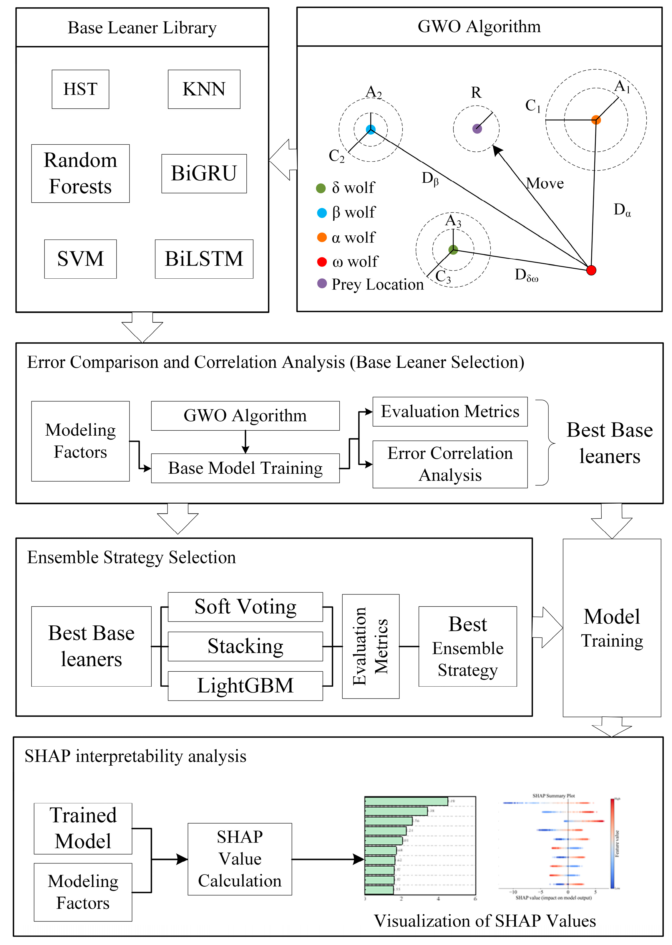
In the context of concrete arch dam deformation prediction, model performance is influenced by a wide range of complex factors. However, significant differences often exist among various base models in terms of predictive accuracy and error distribution. Blindly aggregating such models may lead to degraded performance. To address this issue, this study systematically compares the predictive performance of multiple models on the arch dam deformation task and analyzes the correlation characteristics of their prediction residuals, aiming to identify potential complementarities in their predictive mechanisms. Representative models are then selected to construct a multi-level ensemble learning framework to enhance overall prediction performance. The modeling workflow is illustrated in Figure 8, and the detailed procedure is as follows:
  • Data Preprocessing: Outlier detection and missing value interpolation are applied to both displacement monitoring data and corresponding environmental variables to ensure data completeness and accuracy. All input features are subsequently normalized.
  • Construction of Modeling Factors: Based on engineering experience, a total of 30 influencing factors—primarily including water pressure, temperature, and time-effect components—are selected for model development.
  • Residual Correlation Analysis of Base Models: The correlation coefficients between the prediction residuals of different base models are calculated to assess model complementarity, providing a foundation for subsequent model grouping and ensemble design.
  • Selection of Ensemble Strategies: Three ensemble strategies—Bayesian Model Averaging (BMA), Stacking, and LightGBM-based integration—are pre-defined. Model combinations are determined based on residual correlation analysis, and the optimal ensemble method is selected according to overall fitting accuracy.
  • Construction of the Ensemble-Based Displacement Prediction Model: Representative base models are integrated using the selected ensemble strategy to construct a predictive model capable of accurately forecasting arch dam displacements.
  • SHAP-Based Interpretability Analysis: The SHAP algorithm is employed to quantify the influence of each input factor on the model output, thereby enhancing interpretability and supporting engineering diagnosis and decision-making.

3.2. Prediction Evaluation Metrics

To comprehensively evaluate the predictive performance of the model in the regression task, three commonly used metrics are employed in this study: Root Mean Squared Error (RMSE), Coefficient of Determination (R2), and Mean Absolute Error (MAE).
RMSE measures the standard deviation of the errors between the predicted values and the actual values. The specific formula is as follows:
R M S E = 1 n i = 1 n y ^ i y i 2
R2 measures the goodness of fit of the model. The closer its value is to 1, the better the model’s fit. The specific formula is as follows:
R 2 = 1 i = 1 n y ^ i y i 2 i = 1 n y i ¯ y i 2
MAE represents the average absolute deviation between the predicted values and the actual values, providing an intuitive measure of the average deviation of the predictions. The formula is as follows:
M A E = 1 n i = 1 n y ^ i y i
In the above formula, n represents the sample size, y i denotes the actual value, y ^ i represents the predicted value, and y i ¯ is the mean of the actual values.

4. Engineering Applications

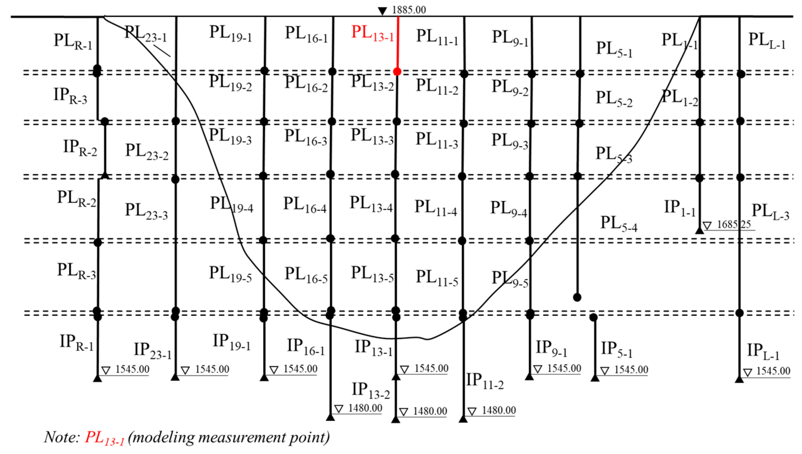
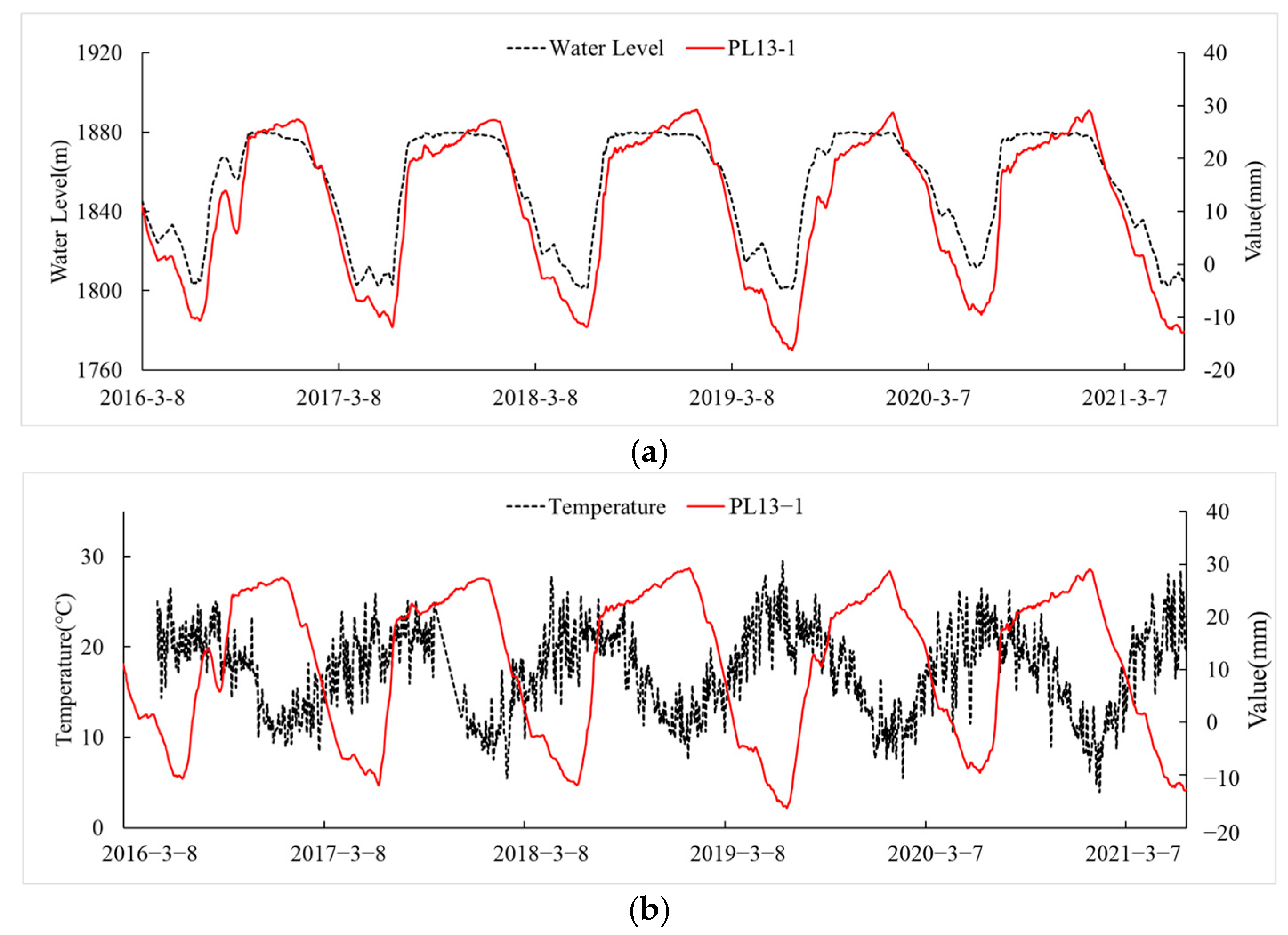
Based on the aforementioned methodology, a composite displacement prediction model is developed using a representative arch dam as a case study. The dam has a crest elevation of 1885.0 m and a maximum height of 305 m. Horizontal displacements are monitored using vertical plumb lines, and the layout of the monitoring system is shown in Figure 9. For model development and analysis, data from monitoring point PL13-1, located at the crown cantilever beam, are selected. Figure 10 illustrates the time series of measured displacements at the monitoring point, upstream reservoir water levels, and toe temperatures. It can be observed that dam displacement exhibits a strong correlation with upstream water level, while toe temperature demonstrates an annual periodic variation.

4.1. Construction of the Ensemble Learning Model

4.1.1. Optimization and Selection of Base Learners

To validate the rationality of the selected base learners in the ensemble learning framework, this study first analyzes the prediction accuracy and residual correlation of different individual models. Six standalone prediction models—including HST model, RF model, KNN model, SVM, BiLSTM, and BiGRU—are each optimized using the GWO algorithm and trained independently. A total of 1936 data samples from monitoring point PL13-1, recorded between 8 March 2016 and 25 June 2021, are used for model development. Of these, 80% of the data are used as the training set and 20% as the testing set. The predictive performance of each model is evaluated and compared based on its individual forecasting results.
The factors involved in modeling are divided as follows: water level-related factors are represented by H j k ( j = 5 i , i = 1 ~ 6 , k = 1 ~ 4 ), H j _ a v g k ( j = 5 i , i = 1 ~ 6 , k = 1 ~ 4 ), where H represents the water level on the current day, and H j denotes the average water depth in front of the dam on the previous j day. H j _ a v g represents the average water depth in front of the dam j days prior. Temperature-related factors are represented by two sets of periodic functions: sin 2 π i 365 t sin 2 π i 365 t 0 , cos 2 π i 365 t cos 2 π i 365 t 0   ( i = 1 ~ 2 ). Time-dependent factors are represented by linear and logarithmic factors: θ θ 0 , ln θ ln θ 0 , where θ = t 100 , θ 0 = t 0 100 , and t are the cumulative days from the monitoring day to the start of monitoring, and t 0 is the cumulative days from the start of monitoring to the first measurement day.
Firstly, the GWO algorithm is used to optimize the hyperparameters of each base model, with the search range as shown in Table 1:
To further corroborate the efficacy of the Grey Wolf Optimizer (GWO), we adopted the hyper-parameter tuning of the baseline BiGRU model as a representative case; the corresponding training trajectory is depicted in Figure 11. As evidenced by the figure, the training-set loss curve produced by GWO descends most precipitously and reaches the lowest asymptote among all comparator methods, attesting to the algorithm’s superior optimization capability. Moreover, the GWO-driven loss stabilizes at a markedly low level after only seven iterations, highlighting the efficiency of the training process. Collectively, these observations confirm the practicability of employing GWO for hyper-parameter optimization of the aforementioned base model.
Upon optimization of all baseline models via the Grey Wolf Optimizer and the completion of training, the performance metrics for each model are summarized in Table 2.
As evidenced by the table, each model attains a modest training error as well as a comparatively small forecasting error. Nevertheless, the predictive prowess of an ensemble hinges critically on the heterogeneity of its base learners—incorporating distinct model archetypes is an effective means of curtailing residual error. Accordingly, in addition to benchmarking raw accuracy, it is indispensable to quantify inter-model dissimilarity. To this end, we evaluate the pairwise Pearson correlation coefficients among the prediction residuals of all candidate models; the resulting analysis is displayed in Figure 12.
In aggregate, Figure 12 and Table 2 show that the RF, SVM and KNN learners achieve the highest individual accuracies. However, these models share a common foundation in traditional machine learning, and their residual-error structures exhibit strong correlations. This indicates that their errors are likely to be highly similar, and as such, including more than one of them in the ensemble would introduce redundancy without substantial improvement in predictive performance. Therefore, to avoid overfitting and maintain diversity in the model ensemble, only the most accurate of the three—the Random Forest (RF)—is retained as a base learner. Similarly, the BiLSTM and BiGRU models are both deep learning architectures, and their residual errors are moderately correlated (Pearson r = 0.716). While these architectures are based on different types of neural networks, the correlation suggests that they share similar patterns in prediction errors. Given its superior predictive accuracy, the BiGRU model is selected as the representative deep-learning model for the ensemble. The HST model, constructed using stepwise regression, shows relatively lower goodness-of-fit compared to the other models. However, its distinctive strengths lie in feature selection and interpretability, which are crucial in many practical applications. The HST model’s ability to provide insights into the importance of individual features and its transparency in decision-making processes make it an invaluable addition to the ensemble. Its inclusion enhances the ensemble’s robustness and introduces valuable methodological diversity, ensuring that the final model is not only accurate but also interpretable.
In summary, weighing both the inter-model error correlations and individual predictive accuracies, we designate the RF, BiGRU, and HST models as the ensemble’s base learners. The hyper-parameter configurations obtained after GWO-based tuning are presented in Table 3.

4.1.2. Selection of Meta-Learners

Building on ensemble-learning principles, we analysed 1936 observations recorded at monitoring point PL13-1 between 8 March 2016 and 25 June 2021. Employing the train–test split outlined in Section 4.1.1, we trained the optimally tuned RF, BiGRU, and HST base learners. Their predictions were then synthesised via three complementary ensemble schemes—soft voting, stacking, and LightGBM—to yield the final forecasts. The comparative predictive accuracies achieved by these strategies are depicted in Figure 13.
Figure 13 demonstrates that the ensemble employing a stacking strategy delivers the highest predictive accuracy among the alternatives; accordingly, stacking is selected as the ensemble-learning framework for this study.

4.1.3. Evaluation of Ensemble Learning Models

Building on the foregoing analysis, the computed evaluation metrics for each model’s forecasts are consolidated in Table 4. The train-test split is identical to that described in Section 4.1.1.
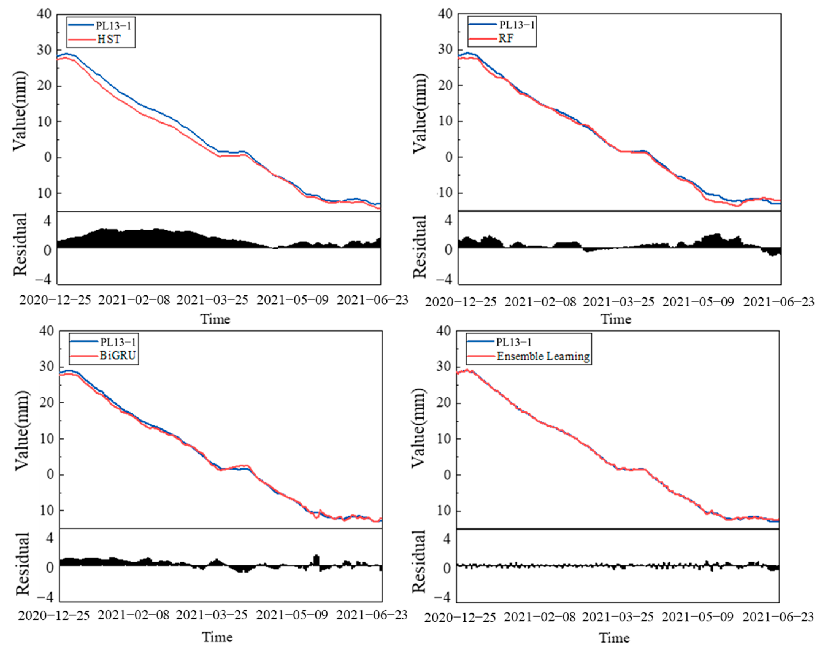
Table 4 indicates that the stacking-based ensemble attains the highest predictive fidelity, yielding an RMSE of 0.2241 and an R2 of 0.9993. Its overall accuracy surpasses that of every constituent base learner, demonstrating that—within the present arch-dam displacement-forecasting task—the ensemble markedly outperforms any single model. In addition, visual comparison of the predicted trajectories with the observed measurements in Figure 14 reveals that:
Although the HST model (derived via stepwise regression) faithfully reproduces the long-term trend of the monitoring series, it proves inadequate at resolving fine-grained fluctuations. The RF learner, representing the machine-learning cohort, captures short-term variability more effectively than HST, yet non-negligible deviations from the observations persist. The BiGRU network emerges as the most competent of the individual models; however, its fit deteriorates when the data display abrupt oscillations. By contrast, the proposed stacking-based ensemble yields predictions that align most closely with the measured values across the entire data set.

4.1.4. Interpretation of Model Prediction Results

After deriving the dam-displacement forecasts with the proposed ensemble model, we elucidated the model’s behavior using SHAP. Figure 15a,b display, respectively, the ranked feature-importance bar chart and the feature-density scatter plot for monitoring point PL13-1.
In Figure 15b, the colour bar to the right encodes the magnitude of each explanatory variable, whereas the abscissa quantifies the corresponding Shapley contribution to the predicted displacement. Inspection of the feature-importance ranking in Figure 15a reveals that nine of the ten most influential covariates are water-level descriptors, underscoring that the dam’s radial displacement is governed predominantly by hydraulic load. Consistent with Figure 10, the displacement exhibits a pronounced correlation with the reservoir stage. Notably, two of the five foremost predictors—H5AVG and H30—represent antecedent water-level indices, implying a discernible lag effect: even when the reservoir remains at a sustained high stage and ambient temperature is comparatively steady, the dam continues to deform gradually (see Figure 10). The temperature harmonic term also exerts a tangible influence, a consequence of the marked, quasi-periodic thermal fluctuations characteristic of the dam’s climatic setting. Finally, the horizontal span of the SHAP values in Figure 15b is greatest for H0, confirming that this variable wields the largest marginal impact on the ensemble’s output.

5. Conclusions and Discussion

This study proposes an interpretable arch-dam displacement prediction framework that combines an ensemble-learning architecture with GWO algorithm-based hyper-parameter tuning. The approach overcomes the limitations inherent in any single-model formulation. By surveying extant displacement-forecasting methodologies, selecting three representative base learners—HST, RF, and BiGRU—and optimising their hyper-parameters via GWO algorithm, the resulting ensemble not only improves predictive accuracy but also enhances model interpretability. Extensive comparative experiments substantiate the method’s efficacy. The principal findings are as follows:
  • The proposed ensemble-learning framework synergistically integrates the merits of multiple base learners. Employing a stacking architecture, it capitalizes on inter-model complementarity and delivers a marked enhancement in the accuracy of arch-dam displacement predictions. AI and ML algorithms, particularly the BiGRU and RF models, demonstrated their effectiveness in anticipating displacement patterns by capturing nonlinear relationships and temporal dependencies that traditional models struggle with.
  • GWO algorithm-based hyper-parameter tuning endows each constituent model with near-optimal training conditions while curtailing computational overhead. This procedure secures peak performance for every learner and appreciably shortens the overall training time.
  • Coupling the ensemble with SHAP analysis renders the model transparently interpretable. The Shapley values unveil the relative contributions of individual influencing factors, thereby reinforcing the model’s practical utility and engineering reliability.
Despite these achievements, several avenues remain for further improvement:
  • Advanced deep-learning architectures. Future studies might incorporate state-of-the-art paradigms—such as Transformers or graph neural networks—as base learners and refine the ensembling strategy to unlock additional predictive gains.
  • Distributed computation. Rising computational power could be harnessed through efficient distributed-learning schemes, expediting the training process and enlarging the ensemble’s operational envelope.
In summary, subsequent research may broaden the application of this methodology to diverse dam-monitoring contexts, experiment with richer families of ensemble and deep-learning algorithms, and thereby confront increasingly complex engineering-prediction challenges while advancing the discipline of structural health monitoring. Additionally, future studies could explore the integration of multiple sensor data to enhance modeling accuracy, investigate the potential of modeling with various sensor types, and incorporate finite element models to guide the modeling process. These approaches could be further refined by combining physical principles with data-driven techniques, offering more robust and interpretable predictive models for structural health monitoring.

Author Contributions

S.L.: Conceptualization, Investigation, Methodology, Software, Writing—original draft, Writing—Review and Editing. K.J.: Project administration, Visualization. S.Y.: Project administration, Visualization. Z.L.: Resources, Supervision, Project administration, Funding acquisition, Writing—Review and Editing. Y.Q.: Conceptualization, Investigation, Formal analysis, Data curation. H.S.: Supervision, Project administration, Funding acquisition, Writing—Review and Editing. All authors have read and agreed to the published version of the manuscript.

Funding

This research has been partially supported by the National Key Research and Development Program of China (2024YFC3210701), the National Natural Science Foundation of China (52239009), and the Independent research project of Yellow River Engineering Consulting Co., Ltd. (2025KY026(2)).

Data Availability Statement

The data that support the findings of this study are available from the corresponding author upon request. The data used in this study contain sensitive information related to the high-arch dam and cannot be shared publicly due to privacy and authority restrictions.

Conflicts of Interest

Authors Shasha Li, Kai Jiang, Shunqun Yang, Zuxiu Lan and Yining Qi are employed by Yellow River Engineering Consulting Co., Ltd. The remaining authors declare that the research was conducted in the absence of any commercial or financial relationships that could be construed as a potential conflict of interest.

References

  1. Li, B.; Yang, J.; Hu, D. Dam monitoring data analysis methods: A literature review. Struct. Control Health Monit. 2019, 27, e2501. [Google Scholar] [CrossRef]
  2. Wen, Z.; Zhou, R.; Su, H. MR and stacked GRUs neural network combined model and its application for deformation prediction of concrete dam. Expert Syst. Appl. 2022, 201, 117272. [Google Scholar] [CrossRef]
  3. Cheng, M.-Y.; Cao, M.-T.; Huang, I.F. Hybrid artificial intelligence-based inference models for accurately predicting dam body displacements: A case study of the Fei Tsui dam. Struct. Health Monit. Int. J. 2022, 21, 1738–1756. [Google Scholar] [CrossRef]
  4. Mata, J.; Tavares de Castro, A.; Sá da Costa, J. Constructing statistical models for arch dam deformation. Struct. Control Health Monit. 2014, 21, 423–437. [Google Scholar] [CrossRef]
  5. Belmokre, A.; Mihoubi, M.K.; Santillan, D. Analysis of Dam Behavior by Statistical Models: Application of the Random Forest Approach. Ksce J. Civ. Eng. 2019, 23, 4800–4811. [Google Scholar] [CrossRef]
  6. Li, M.; Ren, Q.; Li, M.; Qi, Z.; Tan, D.; Wang, H. Multivariate probabilistic prediction of dam displacement behaviour using extended Seq2Seq learning and adaptive kernel density estimation. Adv. Eng. Inform. 2025, 65, 103343. [Google Scholar] [CrossRef]
  7. Liu, X.; Li, Z.; Sun, L.; Khailah, E.Y.; Wang, J.; Lu, W. A critical review of statistical model of dam monitoring data. J. Build. Eng. 2023, 80, 108106. [Google Scholar] [CrossRef]
  8. Papaleontiou, C.G.; Tassoulas, J.L. Evaluation of dam strength by finite element analysis. Earthq. Struct. 2012, 3, 457–471. [Google Scholar] [CrossRef]
  9. Total stress rapid drawdown analysis of the Pilarcitos Dam failure using the finite element method. Front. Struct. Civ. Eng. 2014, 8, 115–123. [CrossRef]
  10. Sun, D.; Zhang, G.; Wang, K.; Yao, H. 3D Finite Element Analysis on a 270 m Rockfill Dam Based on Duncan-Chang E-B Model. In Proceedings of the International Conference on Advanced Engineering Materials and Technology (AEMT2011), Sanya, China, 29–31 July 2011; pp. 1213–1216. [Google Scholar]
  11. Zhu, X.; Wang, X.; Li, X.; Liu, M.; Cheng, Z. A New Dam Reliability Analysis Considering Fluid Structure Interaction. Rock Mech. Rock Eng. 2018, 51, 2505–2516. [Google Scholar] [CrossRef]
  12. Wei, B.; Chen, L.; Li, H.; Yuan, D.; Wang, G. Optimized prediction model for concrete dam displacement based on signal residual amendment. Appl. Math. Model. 2020, 78, 20–36. [Google Scholar] [CrossRef]
  13. Chen, S.; Gu, C.; Lin, C.; Zhang, K.; Zhu, Y. Multi-kernel optimized relevance vector machine for probabilistic prediction of concrete dam displacement. Eng. Comput. 2021, 37, 1943–1959. [Google Scholar] [CrossRef]
  14. Ren, Q.; Li, M.; Kong, R.; Shen, Y.; Du, S. A hybrid approach for interval prediction of concrete dam displacements under uncertain conditions. Eng. Comput. 2023, 39, 1285–1303. [Google Scholar] [CrossRef]
  15. Yu, X.; Li, J.; Kang, F. A hybrid model of bald eagle search and relevance vector machine for dam safety monitoring using long-term temperature. Adv. Eng. Inform. 2023, 55, 101863. [Google Scholar] [CrossRef]
  16. He, P.; Pan, J.; Li, Y. Long-term dam behavior prediction with deep learning on graphs. J. Comput. Des. Eng. 2022, 9, 1230–1245. [Google Scholar] [CrossRef]
  17. Xiong, F.; Wei, B.; Xu, F.; Zhou, L. Deterministic combination prediction model of concrete arch dam displacement based on residual correction. Structures 2022, 44, 1011–1024. [Google Scholar] [CrossRef]
  18. Zhang, C.; Fu, S.; Ou, B.; Liu, Z.; Hu, M. Prediction of Dam Deformation Using SSA-LSTM Model Based on Empirical Mode Decomposition Method and Wavelet Threshold Noise Reduction. Water 2022, 14, 3380. [Google Scholar] [CrossRef]
  19. Yuan, D.; Gu, C.; Wei, B.; Qin, X.; Xu, W. A high-performance displacement prediction model of concrete dams integrating signal processing and multiple machine learning techniques. Appl. Math. Model. 2022, 112, 436–451. [Google Scholar] [CrossRef]
  20. Yu, X.; Li, J.; Kang, F. SSA optimized back propagation neural network model for dam displacement monitoring based on long-term temperature data. Eur. J. Environ. Civ. Eng. 2023, 27, 1617–1643. [Google Scholar] [CrossRef]
  21. Huang, B.; Kang, F.; Li, J.; Wang, F. Displacement prediction model for high arch dams using long short-term memory based encoder-decoder with dual-stage attention considering measured dam temperature. Eng. Struct. 2023, 280, 115686. [Google Scholar] [CrossRef]
  22. Bui, K.-T.T.; Torres, J.F.; Gutierrez-Aviles, D.; Nhu, V.-H.; Bui, D.T.; Martinez-Alvarez, F. Deformation forecasting of a hydropower dam by hybridizing a long short-term memory deep learning network with the coronavirus optimization algorithm. Comput. Aided Civ. Infrastruct. Eng. 2022, 37, 1368–1386. [Google Scholar] [CrossRef]
  23. Yuan, D.; Gu, C.; Wei, B.; Qin, X.; Gu, H. Displacement behavior interpretation and prediction model of concrete gravity dams located in cold area. Struct. Health Monit. Int. J. 2022, 22, 2384–2401. [Google Scholar] [CrossRef]
  24. Zhang, Y.; Zhang, W.; Li, Y.; Wen, L.; Sun, X. A multi-output prediction model for the high arch dam displacement utilizing the VMD-DTW partitioning technique and long-term temperature. Expert Syst. Appl. 2025, 267, 126135. [Google Scholar] [CrossRef]
  25. Li, M.; Pan, J.; Liu, Y.; Wang, Y.; Zhang, W.; Wang, J. Dam deformation forecasting using SVM-DEGWO algorithm based on phase space reconstruction. PLoS ONE 2022, 17, e0267434. [Google Scholar] [CrossRef]
  26. Liu, D.; Yang, H.; Lu, C.; Ruan, S.; Jiang, S. Prediction of displacement of tailings dams based on MISSA-CNN-BiLSTM model. China Saf. Sci. J. (CSSJ) 2024, 34, 145–154. [Google Scholar]
  27. Song, C. A novel stability discriminant model of landslide dams based on CNN-BiGRU optimized by attention mechanism. Landslides 2025, 1–15. [Google Scholar] [CrossRef]
  28. Wu, W.; Su, H.; Feng, Y.; Zhang, S.; Zheng, S.; Cao, W.; Liu, H. A Novel Artificial Intelligence Prediction Process of Concrete Dam Deformation Based on a Stacking Model Fusion Method. Water 2024, 16, 1868. [Google Scholar] [CrossRef]
  29. Liu, M.; Wen, Z.; Su, H. Deformation prediction based on denoising techniques and ensemble learning algorithms for concrete dams. Expert Syst. Appl. 2024, 238, 122022. [Google Scholar] [CrossRef]
  30. Wang, R.; Bao, T.; Li, Y.; Song, B.; Xiang, Z. Combined prediction model of dam deformation based on multi-factor fusion and Stacking ensemble learning. J. Hydraul. Eng. 2023, 54, 497–506. [Google Scholar]
  31. Chithuloori, P.; Kim, J.-M. Soft voting ensemble classifier for liquefaction prediction based on SPT data. Artif. Intell. Rev. 2025, 58, 228. [Google Scholar] [CrossRef]
  32. Liu, M.; Feng, Y.; Yang, S.; Su, H. Dam Deformation Prediction Considering the Seasonal Fluctuations Using Ensemble Learning Algorithm. Buildings 2024, 14, 2163. [Google Scholar] [CrossRef]
  33. Yu, H.; Wang, X.; Ren, B.; Zheng, M.; Wu, G.; Zhu, K. IAO-XGBoost ensemble learning model for seepage behavior analysis of earth-rock dam and interpretation of prediction results. J. Hydraul. Eng. 2023, 54, 1195–1209. [Google Scholar]
  34. Luo, H.; Guo, S.; Bao, W. Random forest model and application of arch dam’s deformation monitoring and prediction. South-to-North Water Transf. Water Sci. Technol. 2016, 14, 116–121. [Google Scholar]
  35. Fang, C.; Jiao, Y.; Wang, X.; Lu, T.; Gu, H. A Dam Displacement Prediction Method Based on a Model Combining Random Forest, a Convolutional Neural Network, and a Residual Attention Informer. Water 2024, 16, 3687. [Google Scholar] [CrossRef]
  36. Wang, X.; Zhu, K.; Yu, H.; Cai, Z.; Wang, C. Combinatorial deep learning prediction model for dam seepage pressure considering spatiotemporal correlation. J. Hydroelectr. Eng. 2023, 42, 78–91. [Google Scholar]
  37. Mirjalili, S.; Mirjalili, S.M.; Lewis, A. Grey Wolf Optimizer. Adv. Eng. Softw. 2014, 69, 46–61. [Google Scholar] [CrossRef]
  38. Lundberg, S.M.; Lee, S.-I. A Unified Approach to Interpreting Model Predictions. In Proceedings of the 31st Annual Conference on Neural Information Processing Systems (NIPS), Long Beach, CA, USA, 4–9 December 2017. [Google Scholar]
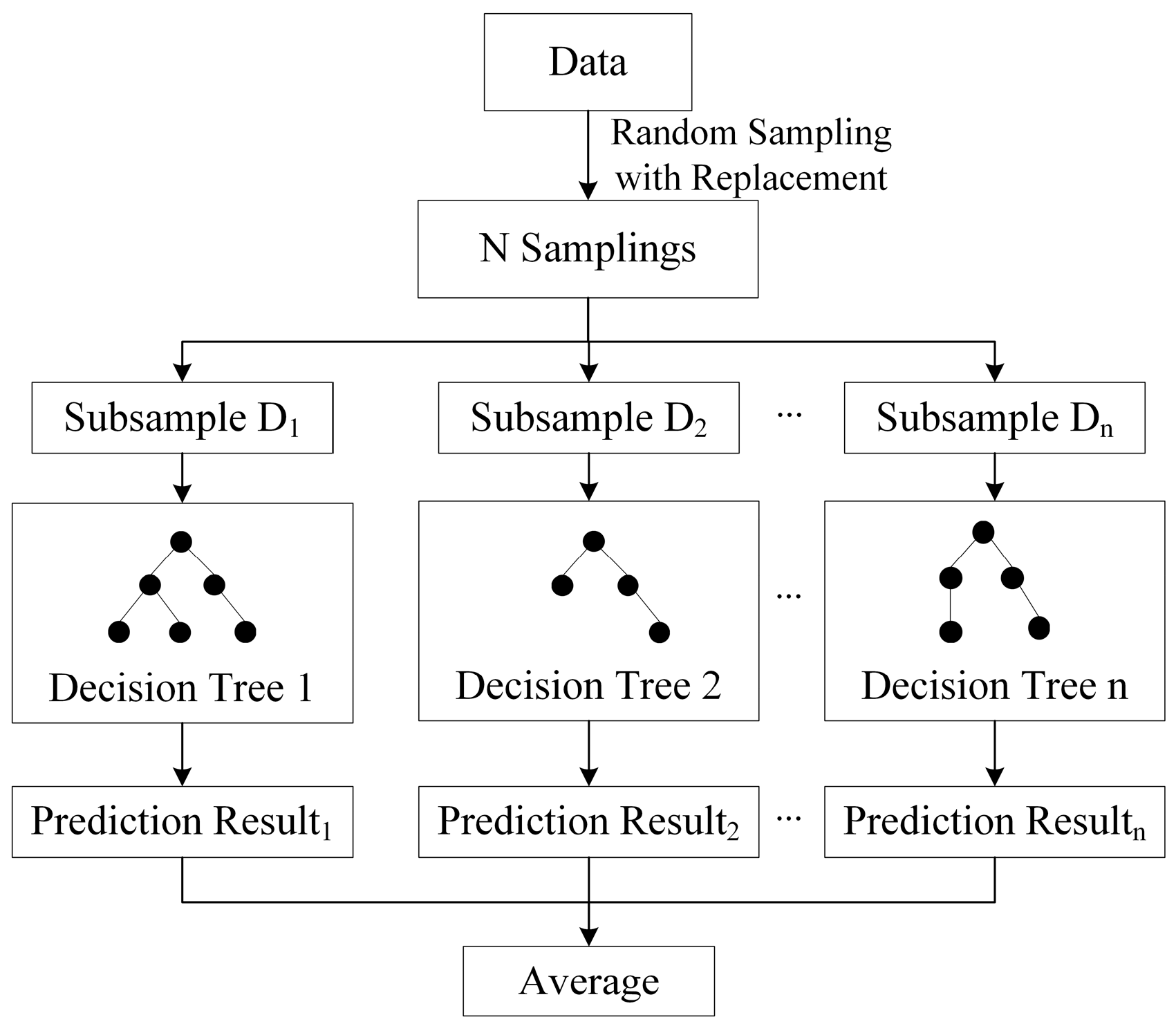
Figure 1. Basic Principle of Random Forest Algorithm.
Water 17 02766 g001
Figure 2. SVM Principle: Linear Separation in 2D and 3D Spaces.
Water 17 02766 g002
Figure 3. KNN Model Principle Diagram.
Water 17 02766 g003
Figure 4. Bidirectional Long Short-Term Memory Network Architecture.
Water 17 02766 g004
Figure 5. Long Short-Term Memory Network Architecture.
Water 17 02766 g005
Figure 6. Gated Recurrent Unit Architecture.
Water 17 02766 g006
Figure 7. Ensemble Strategy Diagram.
Water 17 02766 g007
Figure 8. Model Workflow Diagram.
Water 17 02766 g008
Figure 9. Dam Vertical Line Measurement Point Layout Diagram.
Water 17 02766 g009
Figure 10. The measurement values at point PL13-1 and the corresponding environmental parameters process curve of the dam. (a) The measurement values at point PL13-1 and the corresponding upstream water level process curve. (b) The measurement values at point PL13-1 and the corresponding temperature process curve.
Water 17 02766 g010
Figure 11. Loss Value Variation Curve.
Water 17 02766 g011
Figure 12. Correlation Analysis of Prediction Errors for Each Model.
Water 17 02766 g012
Figure 13. Radar Chart of Evaluation Metrics for Different Meta-Learning Strategies.
Water 17 02766 g013
Figure 14. Comparison of Prediction Results Between Base Models and the Ensemble Model.
Water 17 02766 g014
Figure 15. Multi-Method Comparative Analysis of Model Factor Feature Importance, they should be listed as: (a) Feature Importance Score Bar Chart, (b) Feature Density Scatter Plot for Monitoring Point PL13-1.
Water 17 02766 g015
Table 1. Hyperparameter Optimization Ranges for Each Base Model Table.
ModelModel Hyperparameter Search Range
RFEstimators number [50, 100, 150, 200, 300]; max depth [None, 5, 10, 15, 20]
min samples split [2, 5, 10, 20]; min samples leaf [1, 2, 4, 8]
SVMC [0.1, 1, 10, 100]
KNNNeighbors number [3, 5, 7, 9, 11, 15, 20]; weights [‘uniform’, ‘distance’]
BiLSTMUnits [50, 100, 200, 300]; dropout [0.0, 0.1, 0.2, 0.3, 0.5];
Batch size [16, 32, 64, 128]; learning rate [0.001, 0.01, 0.1]
BiGRUUnits [50, 100, 200, 300]; dropout [0.0, 0.1, 0.2, 0.3, 0.5];
Batch size [16, 32, 64, 128]; learning rate [0.001, 0.01, 0.1]
Table 2. Performance Evaluation Metrics for Each Base Model.
ModelTrain Data AccuracyTest Data Accuracy
RMSEMAER2RMSEMAER2
HST1.06400.55490.99720.71580.53350.9865
RF0.71450.40420.99850.52880.46460.9985
SVM0.83220.35830.99840.53350.40100.9642
KNN0.84680.20790.99930.34500.21110.9856
BiLSTM0.98810.30530.99890.45490.38280.9908
BiGRU0.64090.27350.99910.40880.23770.9941
Table 3. Optimized Hyperparameters for Selected Base Models.
ModelModel Optimal Hyperparameters
RFEstimators number: 200; max depth: 10 min samples split: 5; min samples leaf: 2
BiGRUUnits: 200; dropout: 0.3; Batch size: 64; learning rate: 0.01
Table 4. Table of Performance Evaluation Metrics for Each Model.
ModelTest Data Accuracy
RMSEMAER2
HST0.71580.53350.9865
RF0.52880.46460.9985
BiGRU0.40880.23770.9941
Ensemble Learning0.22410.23470.9993
Disclaimer/Publisher’s Note: The statements, opinions and data contained in all publications are solely those of the individual author(s) and contributor(s) and not of MDPI and/or the editor(s). MDPI and/or the editor(s) disclaim responsibility for any injury to people or property resulting from any ideas, methods, instructions or products referred to in the content.