Article

Water Demand Prediction Model of University Park Based on BP-LSTM Neural Network

1
Research Center of Fluid Machinery Engineering and Technology, Jiangsu University, Zhenjiang 212013, China
2
School of Marine Equipment Engineering, Jiangsu University, Zhenjiang 212013, China
*
Author to whom correspondence should be addressed.
Water 2025, 17(18), 2729; https://doi.org/10.3390/w17182729
Submission received: 4 August 2025 / Revised: 4 September 2025 / Accepted: 11 September 2025 / Published: 15 September 2025

Abstract

Accurate water demand prediction is essential for optimizing the daily operations of water treatment plants and pumping stations. To achieve accurate prediction of water demand for university campuses, this study utilizes real hourly water consumption data collected over 380 observation days from a water treatment plant located on a university campus in Zhenjiang, Jiangsu Province. Based on periodicity analysis of the original data through Fast Fourier Transform (FFT) and autocorrelation coefficients, the data were preprocessed and aggregated into two-hour intervals. The processed water consumption data, along with temporal information (month, day of the week, date, and hour) and weather conditions (daily average wind speed, maximum and minimum temperature), were used as model inputs. The first 352 days of data were utilized to train the model, followed by 14 days serving as the validation set and the final two weeks as the test set. A hybrid forecasting model for campus water demand was developed by integrating a Back Propagation (BP) neural network with a Long Short-Term Memory (LSTM) neural network. The model’s performance was compared with standalone BP, LSTM, and Seasonal Autoregressive Integrated Moving Average (SARIMA) models. Simulation results demonstrate that, compared to other models, the proposed BP–LSTM hybrid model achieves a reduction in Mean Absolute Percentage Error (MAPE) ranging from 4.4% to 15.8%, and a decrease in Root Mean Squared Error (RMSE) between 2.5% and 16.8%. These findings indicate that the BP–LSTM model offers higher prediction accuracy and greater reliability compared to traditional single-model approaches.

1. Introduction

With the development of industrialization, population growth, and the impacts of climate change, water demand continues to increase. A reliable water supply system is essential for the rational allocation and efficient management of water resources, directly influencing the stable operation of urban water distribution networks. Developing a high-precision water demand forecasting model can improve the decision-making capability of pump station scheduling, enhance information management technologies, and support more scientific and efficient planning and control [1]. Thus, it promotes the intelligent construction and development of the urban water supply system.
Water demand forecasting is typically categorized into three levels: long-term, medium-term, and short-term. Long-term forecasting, spanning over a decade, provides a foundation for strategic urban planning and development. Medium-term forecasting, conducted on a monthly or yearly basis, offers guidance for water usage policies. Short-term forecasting, usually performed at an hourly or daily resolution, is essential for the efficient operation of water treatment plants and pumping stations. It helps reduce costs while ensuring that regional water demands are met [2].
Traditional forecasting models often rely on statistical methods, such as linear regression, to analyze the relationship between urban water demand and external variables [3]. Miaou (1990) introduced a stepwise time-series regression identification method for water demand prediction, which was later applied to three datasets for comparative analysis [4]. However, they are insufficient in short-term forecasting accuracy. As research shifted toward data-driven approaches, single models such as autoregressive models, v-support vector machines, and Long Short-Term Memory (LSTM) neural networks [5] showed improvements in prediction performance. Chen et al. proposed an autoregressive model with 5–10 parameters. The double-seasonal autoregressive integrated (ARI) models were able to achieve 1 h-ahead forecasts with a mean absolute percentage error (MAPE) of approximately 5%, and 2–10 h-ahead forecasts with a MAPE of less than 11% [6]. Xue et al. proposed a v-support vector machine (v-SVM) for water consumption prediction, which achieved a maximum absolute relative error of 7.8% and a mean absolute percentage error (MAPE) of 3.45% in hourly water demand forecasting [7].
Nevertheless, these methods still struggle to process multi-source coupled-feature data effectively. In response, hybrid models have made notable progress by integrating feature fusion techniques. For example, Chen et al. developed a hybrid model combining wavelet transform and random forest regression to forecast daily urban water consumption in southwestern China. This model reported a MAPE of 6.98 and a normalized root mean square error (NRMSE) of 0.0857 [8]. Iwakin et al. proposed a CNN-BiLSTM architecture to enhance forecasting ability in real-world scenarios. This architecture achieved a prediction accuracy of 94.88% [9]. The former model focused on daily urban water usage, while the latter targeted hourly water consumption in standard residential areas. However, both approaches face limitations in transferring to university campus settings due to substantial differences in water usage magnitude and variability.
The application of deep learning in the water industry remains in its early stages. Most existing studies rely on synthetic data, laboratory-based systems, or pilot-scale platforms to evaluate model performance [10]. Previous research has mainly focused on urban or industrial water demand forecasting, which has more obvious statistical characteristics [11]. However, as a special small area, the campus has unique characteristics such as low data quality, complex periodicity, and severe instantaneous fluctuations. Existing models often lack sufficient transferability, and a single model is generally incapable of simultaneously accounting for both the temporal inertia inherent in time-series data and the influence of external factors [12].
To address the aforementioned issues, this study employs the Augmented Dickey–Fuller (ADF) test and Fast Fourier Transform (FFT) to examine the stability of historical data and analyze its characteristics. The ADF test ensures the stationarity of the time series data, providing a reliable statistical foundation for model construction. The FFT analysis quantitatively identifies the multi-scale physical periodicities inherent in the water demand series. These validated periodic features serve as strong prior information input to the model, effectively reducing the learning difficulty of the neural network and offering a quantitative basis for setting its hyperparameters. Furthermore, to overcome the limitations of existing hybrid models in integrating complex spatiotemporal features and coupling external factors, a BP-LSTM hybrid forecasting framework is proposed to capture the applicability of temporal and spatial relationships between multivariate factors such as user water demand, weather, and calendar information. This is achieved through improvements in neural network architecture and hyperparameter configuration to forecast future water usage data. Subsequently, structural innovations and algorithmic optimizations are introduced to preserve the temporal modeling strengths of LSTM while compensating for the inadequacy of BP networks in capturing spatial feature sensitivities. Finally, the predictive accuracy and reliability of the model are validated using a test set.

2. Data Presentation and Evaluation Method

The water demand data utilized in this study were collected from a university campus located in Zhenjiang, Jiangsu Province. The total water-consuming population of this campus is approximately 50,000, comprising over 45,000 students, approximately 2700 faculty members, and around 2000 administrative and logistics staff. Accordingly, the major water uses can be classified into three categories: domestic consumption, teaching and research activities, and logistics operations. Hourly water demand data were recorded from 1 June 2022 to 15 June 2023, spanning a total of 380 observation days. After preprocessing, the data were aggregated into two-hour intervals. The first 352 days of data were allocated for model training, the subsequent 14 days were used for validation, and the final two weeks served as the test set. The prediction resolution was maintained at two-hour intervals. In addition to water consumption data, this study also utilized temporal information (month, day of the month, day of the week, and hour) and weather conditions (daily average wind speed, maximum temperature, and minimum temperature) in Jingkou District, Zhenjiang City, Jiangsu Province, China, as inputs to the neural network. The meteorological data were obtained from the China Meteorological Administration [13] and compiled by the weather website [14] with a daily resolution. The weather data were provided with a daily resolution.

2.1. Data Processing

Deep learning models iteratively learn optimal network parameters based on historical data to accomplish forecasting tasks such as water demand prediction. The accuracy and quality of historical data significantly influence the model’s predictive performance. Due to hardware limitations of conventional pumping station measurement devices, the historical water consumption data from the university campus exhibit low quality, including missing values and outliers. Data points with water demand substantially lower than that of other periods are identified as invalid. An acceptable range for normal data is defined as values between 0.6 and 1.6 times the mean value. Data points falling outside this acceptable range are classified as erroneous. A moving average method, which accounts for the periodic nature of the data, is employed to estimate and impute both the invalid and erroneous data points in the original dataset [15].
The collected original time series of water demand is shown in Figure 1. As can be seen from Figure 1, the original water demand series has an obvious 24 h periodicity throughout the data range. Based on previous research findings, it is assumed that water demand at a given time is similar to that at the same time on the two preceding and following days, as well as on the same weekday during the two preceding and following weeks [16].
Therefore, the processing steps for missing and abnormal data in the original data are as follows:
(1) Removal of invalid data: By observing the original data, it is found that only a very small number of data are below 50 m3/h, which is much smaller than the water demand at other times. Therefore, data less than 50 m3/h are considered invalid.
(2) Missing value imputation using weighted moving average: A moving average of water demand was calculated based on one-week and one-day cycles, respectively. These two averages were then weighted and combined to fill in the missing values. The specific calculation formula is as follows:
q D t = A ( q ( D 7 ) t + q ( D + 7 ) t 2 ) + ( 1 A ) ( q ( D 1 ) t + q ( D + 1 ) t 2 ) ,
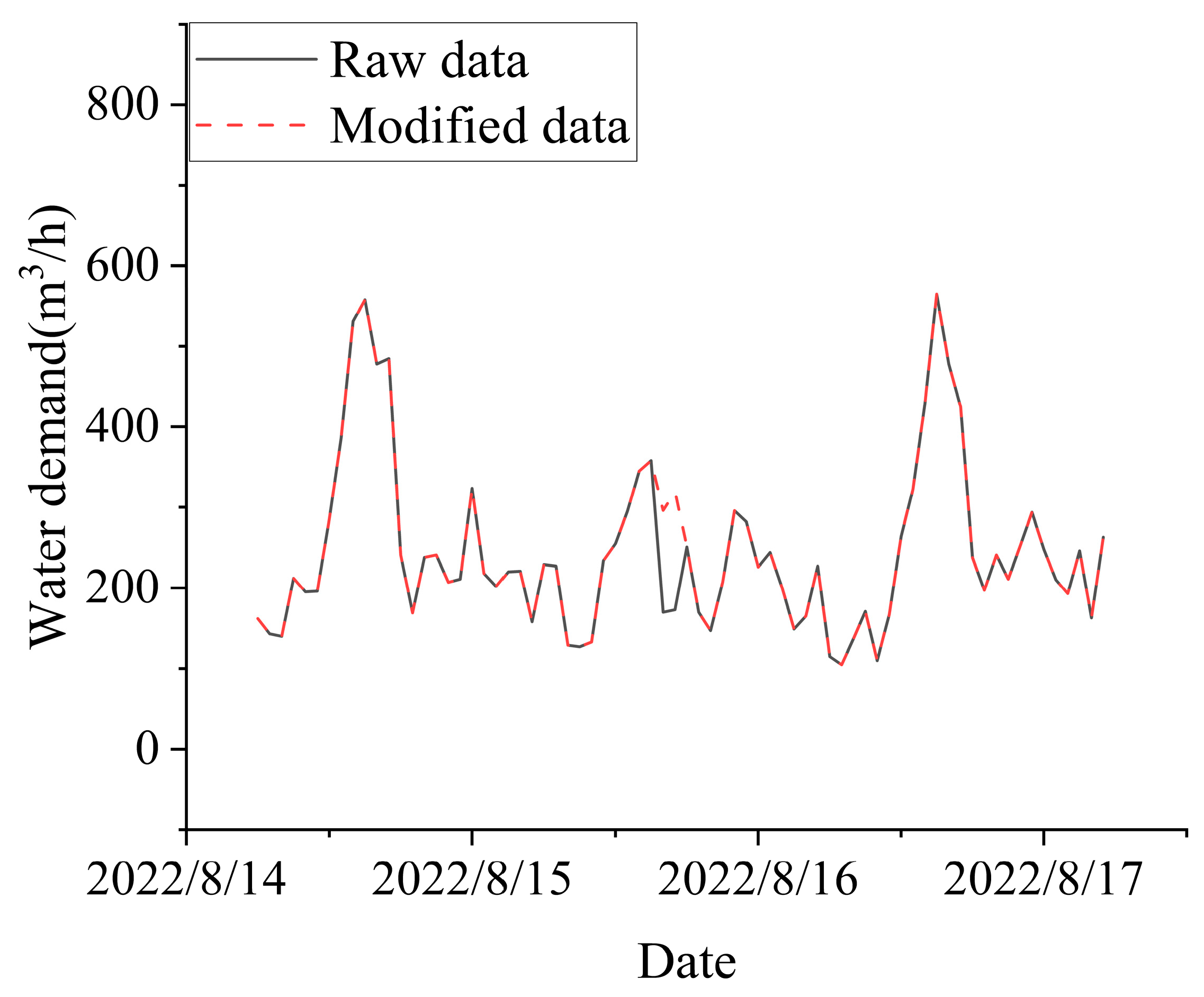
In the equation, qDt represents the water demand on the D-th day and at the t-th hour (t = 0, 1, 2, …, 23) in the data. A is a random weight, which is randomly generated within the range of 0 to 1 using the ‘random’ function in Python 3.9. The filled-in data are shown in Figure 2.
(3) Carrying out the monitoring of abnormal data for the filled data. Abnormal data usually arises due to special circumstances. An excessive amount of abnormal data often indicates that the selected determination conditions are inappropriate. Only the water demand situations during the same time period of two consecutive days are considered, and the determination conditions for abnormal data are adjusted. Based on this comparison, the criteria for identifying abnormal data are iteratively adjusted. Eventually, the acceptable range for normal data is established as 0.6 to 1.6 times the mean value. Under these conditions, a total of 21 data points are identified as abnormal.
These abnormal values were then replaced with random values within the range of 0.9 to 1.1 times the average water demand for the same time period across two consecutive days. Let B be the random coefficient, and the selection method is the same as that of A, an example of this replacement process is illustrated in Figure 3:
q D t = B ( q ( D 1 ) t + q ( D + 1 ) t 2 ) ,
(4) Water demand data are inherently time-series data. Aggregating data over longer time intervals can be achieved by summing the values from adjacent periods. Since water utilities typically estimate demand by calculating the difference between successive meter readings, the aggregated data over larger intervals more accurately reflect the actual water consumption. Meanwhile, to ensure that the model can effectively capture variation patterns in water demand, the temporal resolution should remain comparable to that of the original data. Therefore, the original hourly water demand data—24 data points per day—were aggregated into 12 two-hour intervals per day:
Q D T = q D ( 2 T ) + q D ( 2 T + 1 ) ,
In the equation, QDT represents the water demand for the T-th two-hour period on the D-th day in the data (t = 0, 1, 2, …, 11).

2.2. Data Analysis

Comprehensive data analysis enables the explicit characterization of feature patterns, which in turn guides the optimal selection of input variables and supports the development of customized neural network architectures. This process contributes to improved forecasting accuracy.

2.2.1. Fast Fourier Transform

In signal processing and spectral analysis, the Fourier transform is widely used to convert data from the time domain to the frequency domain, thereby revealing the underlying frequency components and periodic patterns. It is a fundamental tool for key tasks such as analyzing complex time-series data, performing signal decomposition and reconstruction, and facilitating pattern recognition [17].
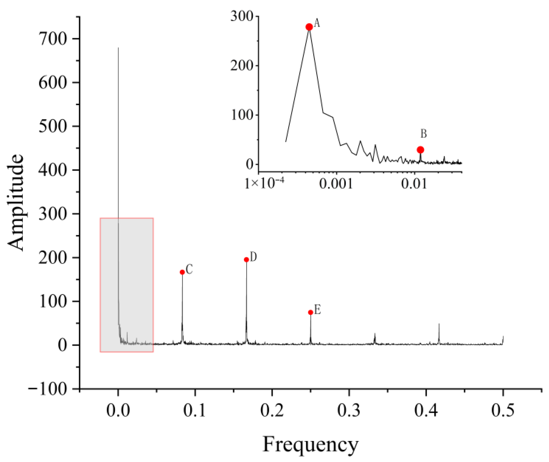
By using the FFT tool in Origin, the processed water demand time-series data with a resolution of 2 h is converted into frequency-domain data. The resulting frequency and amplitude data are presented in Figure 4. Based on these results, the periodic characteristics of the original data were analyzed. The calculation of the actual time periods corresponding to different frequencies is as follows:
T Z = T I f ,
In the equation, TI represents the time interval between two adjacent data points in the original data. Here, it is two hours. f represents the frequency. It can be seen that the amplitudes at the five frequencies from A to E are significantly larger than those at their surrounding frequencies. Although the amplitude at point B is relatively small in absolute terms, it is still markedly greater than those of its adjacent frequencies. The corresponding time periods for frequencies A through E are listed in Table 1.
As shown in Table 1, the water demand data for the university campus exhibit pronounced periodic characteristics. The 186-day cycle (approximately half a year) aligns with the academic semester structure. The one-week cycle is related to the work cycle. The remaining cycles are regarded as the result of the influence of daily work and rest time.

2.2.2. Difference and ADF Tests

Many traditional time series prediction models require the input data to be stationary, meaning that the mean and variance of the time series do not exhibit significant changes over time. The stationarity of data reflects the extent to which past values can be used to predict future values. In this study, the ADF test, also known as the unit root test, is employed. A time series that contains a unit root is considered non-stationary, implying that its statistical properties (such as mean and variance) vary over time [18].
In practical applications, time series data often exhibit trends and seasonality, which contribute to non-stationarity. In such cases, differencing can be applied to the original series to remove trend or seasonal components, thereby transforming the data into a stationary series [19]. The definition is as follows:
X t = Y t + 1 Y t ,
In the formula, Yt represents the original data, and Xt represents the differenced data. The results of the first-order and second-order differencing are illustrated in Figure 5.
The ADF test was performed on three sets of data using the statsmodels module in Python. The corresponding results are shown in Table 2. The T-value indicates the t-statistic obtained from the test, and the p-value denotes the probability associated with the t-statistic.
By comparing the statistical values and the critical T-values for rejecting the null hypothesis at different significance levels, one can observe the p-values. If the T-value is sufficiently small and the p-value is less than 0.05, it indicates that the data strongly rejects the unit root hypothesis and belongs to stationary data. From the above table, the original data are non-stationary, while the data starting from the first-order difference are stationary.

2.2.3. Autocorrelation Coefficient Calculation

After confirming the stationarity of the data, it is necessary to examine whether internal correlation—namely, autocorrelation—exists within the time series, as this reflects the sequential dependency among data points. In this study, the Autocorrelation Function (ACF) is employed to evaluate this aspect. The ACF measures the degree of correlation between current and past observations, thereby quantifying the strength of autocorrelation in the time series [20]. Its definition is given as follows:
ρ k = Cov ( X t , X t k ) Var ( X t ) Var ( X t k ) ,
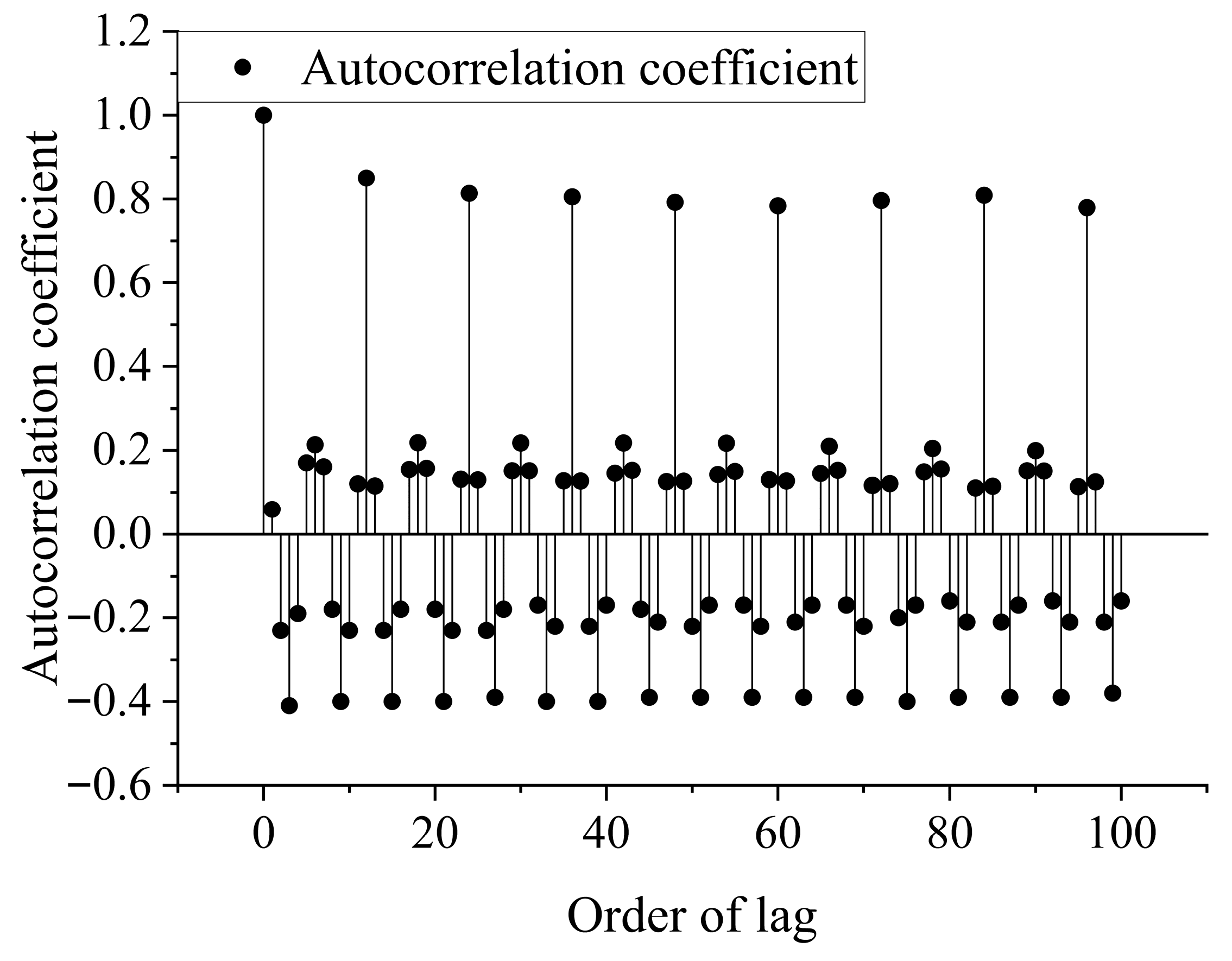
In the formula, k represents the lag order. Cov(Xt, Xt−k) represents the covariance between the time series Xt and Xt−k. Var(Xt) and Var(Xt−k) represent the variances of the time series Xt and Xt−k, respectively. Figure 6 shows the autocorrelation coefficients of the original data after first-order differencing.
As can be seen from Figure 6, the time series with a lag of every 12 steps (24 h) has a relatively strong correlation. Secondly, the correlation with a lag of every 6 steps (12 h) is also more significant. Moreover, an obvious 12-step periodic pattern is presented as a whole. This phenomenon further supports the findings of the FFT analysis.

3. Model and Method

3.1. Seasonal Autoregressive Differential Moving Average Model

The Seasonal Autoregressive Integrated Moving Average (SARIMA) model is an extension of the Autoregressive Integrated Moving Average (ARIMA) model [21]. The traditional ARIMA model, typically denoted as ARIMA (p, d, q), consists of three components:
(1) Autoregressive model (AR): It is used to describe the relationship between the current value and historical values. It predicts itself using historical data. The parameter p indicates the number of lagged terms included in the autoregressive part. The formula for this component is as follows:
X t = μ + i = 1 p γ i X t i + ε t ,
In the equation, μ is a constant, ε t is random noise, and γ i is an autoregressive coefficient.
(2) Differencing (I): This part of the model is associated with the parameter d, which represents the number of differencing operations required to transform the data into a stationary series. As stated in Section 2.2.2, d = 1 in this paper.
(3) Moving Average Model (MA): This component models the dependency between the current observation and past forecast errors. It is used to smooth the data and enhance forecasting accuracy. The parameter q denotes the number of lagged forecast errors included in the moving average part. The corresponding formula is as follows:
X t = μ + i = 1 q θ i ε t i + ε t ,
In the equation, θ i is the moving average coefficient.
The SARIMA model extends the ARIMA model by explicitly capturing the seasonal or periodic components in the data. The SARIMA model is usually written as SARIMA(p, d, q)(P, D, Q)ss. Here, p represents the autoregressive lag length of the series; d is the order of differencing; q is the order of the moving average. P is the seasonal autoregressive lag length of the series; D is the order of seasonal differencing; Q is the seasonal order of moving average; and s is the season length.

3.2. BP-LSTM Combined Model

To enhance the accuracy of water demand forecasting based on the water-use characteristics of university campuses, this study proposes a BP-LSTM forecasting model, which integrates a BP neural network with an LSTM neural network. The LSTM component is designed to capture both long-term and short-term periodic patterns in water consumption [22]. The BP network, on the other hand, analyzes the instantaneous impacts of discrete variables such as sudden weather changes and holidays through non-linear mapping [23]. These two networks are jointly trained in an end-to-end manner, with feature space fusion achieved via dynamic weight allocation within the neural network. The overall structure and data flow of the combined model are illustrated in Figure 7.

3.2.1. BP Neural Network

The BP neural network is a multi-layer feedforward neural network trained using the error backpropagation algorithm. It typically consists of three layers: the input layer, hidden layers, and the output layer [24]. Each hidden layer contains a certain number of neurons. For a single neuron, its input–output formula is as follows:
y i j = f ( n = 1 n ω i j n x ( i 1 ) n + b i j ) ,
In the equation, y i j represents the output of the j-th neuron in the i-th layer. x ( i 1 ) n represents the n-th output of the previous layer. ω i j n is the weight corresponding to the output of the previous layer at the position of this neuron. b i j is the bias corresponding to this neuron. f(x) is the activation function. In this paper, the ReLU function is chosen:
RELU ( x ) = x x > 0 0 x 0 ,
During training, the weights and biases of the neural network are initially initialized using random functions. These parameters are iteratively updated via gradient descent and backpropagation to minimize the discrepancy between predictions and target values. This adaptive learning mechanism addresses the limitations of traditional static weight updates and enhances both the learning efficiency and generalization capability of the model through real-time parameter optimization.
Previous studies [25] have shown that when the temporal resolution of the input layer exceeds that of the forecasting target, the model is better able to capture fluctuations in water demand, thereby improving forecasting accuracy. Considering the periodic nature of the original data, this study selects hourly water consumption data from the 12 h preceding the target time, as well as two-hour water consumption records from the corresponding time period on the previous day and the previous week, as input features. Additionally, target time information and daily weather information are incorporated [26]. The final structure of the input layer is shown in Table 3.

3.2.2. LSTM Neural Network

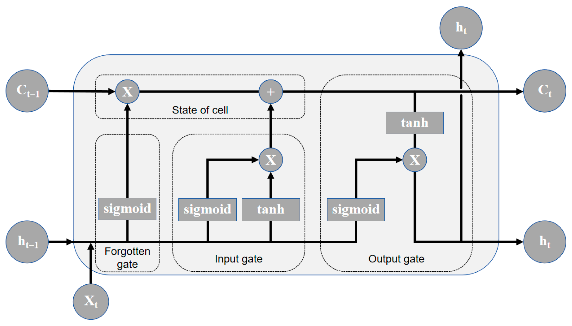
LSTM neural network, a specialized type of Recurrent Neural Network (RNN), has demonstrated exceptional performance in handling sequential data with long-term dependencies. It effectively addresses the issues of gradient vanishing and gradient explosion commonly encountered in traditional RNNs when processing long sequences [27]. LSTM introduces a gating mechanism that regulates the flow of information, thereby optimizing the learning process. It comprises four core components: the input gate, the forget gate, the cell state, and the output gate. The structure is shown in Figure 8. Here, Xt represents the input information, Ct represents the cell state, and ht represents the hidden information.
The forget gate determines which information should be discarded from the current cell state. It employs a sigmoid activation function, which outputs values between 0 and 1 to represent the importance of each piece of information. This enables the LSTM to selectively retain or discard information based on the current input and the previous hidden state.
The input gate decides whether new information should be stored in the cell state. It consists of a sigmoid activation function and a tanh activation function. The sigmoid function evaluates the relevance of the new input, while the tanh function scales the input values to the range of [−1, 1]. These functions work jointly to filter and retain essential input information.
The state of the cell is a key part of the LSTM. It allows information to flow without increasing the computational complexity. It is a linear layer that can read information from the cell state of the previous time step or through the forget gate. This mechanism allows the model to maintain long-term information and avoid gradient-related issues during training.
The output gate determines the next hidden state. It also comprises a sigmoid activation function and a tanh activation function. The sigmoid function controls the significance of the output, while the tanh function extracts part of the cell state. With this, the LSTM can generate output information with appropriate importance according to the current input and the cell state.
By adjusting its internal states in response to the current input and long-term memory, the LSTM is capable of learning complex long-term dependencies in sequential data [28]. Given the periodic characteristics of the original data and referring to the quality of the forecasting effect during the debugging process, the data of the first 96 h, that is, the data of the first four days, are finally selected as the input of the LSTM model.

3.2.3. Ensemble Design

In a combined forecasting model, the determination of weight coefficients for individual forecasting results is of critical importance, as it directly influences the overall forecasting accuracy. These models typically employ a weighted average of the outputs from individual models as the integration approach. A reasonable assignment of weight coefficients can substantially enhance the accuracy of the combined forecasting model, enabling it to more effectively capture patterns and trends by leveraging the strengths of different individual models. Currently, common methods for determining weight coefficients include the arithmetic mean method, the reciprocal method, and methods based on mathematical optimization [29]. In this study, a simple BP neural network with two hidden layers is employed to perform the combination. The forecasting results of the trained BP and LSTM models, along with time information and weather information, are used as the model inputs to obtain the final forecasting result.

3.3. Determine the Hyperparameters of the Model

The hyperparameters of a model play a critical role in determining its performance. Therefore, evaluating different hyperparameter combinations using a validation set and selecting the optimal configuration is essential. Various optimization strategies exist for hyperparameter tuning, including grid search, genetic algorithms, particle swarm optimization, etc. [30]. Considering the scale of tunable hyperparameters of the model and the size of the input layer of each model, this paper chooses the grid search method as the main means of hyperparameter optimization. The hyperparameters are explored and compared within a predefined search space, and the optimal combination is ultimately selected based on performance evaluation.

3.3.1. SARIMA Model Parameters Determination

When constructing the SARIMA model, the intrinsic meanings of its hyperparameters are taken into account. Some parameters can be determined directly based on data analysis results. For example, the seasonal length parameter s is set to 12, as inferred from the periodic pattern identified in Figure 6. Regarding the differencing order d and the seasonal differencing order D, the original data becomes stationary after first-order differencing. Therefore, d = D = 1. For other parameters, the grid search method is adopted, and an optimized selection is carried out according to the Akaike Information Criterion (AIC). The formula is as follows:
A I C = 2 ln ( L ) + 2 α ,
In this equation, L represents the maximum likelihood function under the given model, and α is the number of parameters in the model. Based on the concept of entropy, AIC can comprehensively consider the complexity of the model and the goodness of data fitting. A lower AIC value indicates better model performance. In this study, the statsmodels library in Python is used to compute the AIC values of SARIMA models under various parameter combinations. By comparison, the parameter combination with the minimum AIC value is selected as the final model parameter. Accordingly, SARIMA(5,1,1)(6,1,1)12 is finally determined as the model parameter.

3.3.2. BP-LSTM Model Parameters Determination

Hyperparameter optimization is essential for improving the accuracy and efficiency of neural networks. In this study, for the BP neural network, LSTM neural network, and the combined BP-LSTM model, preliminary training with a small number of epochs is conducted to examine the influence of various hyperparameters, including the number of network layers, the number of neurons in each hidden layer, the learning rate, and the batch size. Based on minimizing the MAPE on the validation set, the hyperparameters for each model are selected using the grid search method. According to the MAPE performance of the three models under different hyperparameter combinations, the final configurations for the BP, LSTM, and BP-LSTM models are determined, as summarized in Table 4.

4. Results and Discussion

4.1. Model Evaluation Metrics

To evaluate the forecasting accuracy of the forecasting model more intuitively, this study selected three key performance indicators: the Coefficient of Determination R2, the Root Mean Squared Error (RMSE), and the Mean Absolute Percentage Error (MAPE) [31,32]. R2 quantifies the goodness of the model fit. Its value ranges from 0 to 1. The closer the value is to 1, the higher the degree of fit. RMSE focuses on measuring the absolute magnitude of the forecasting error, while MAPE concerns the relative proportion between the forecasting error and the actual value. Lower RMSE and MAPE values generally indicate higher forecasting accuracy. These metrics are widely employed in practice to assess the accuracy and reliability of forecasting models. The mathematical definitions of these metrics are presented as follows:
R 2 = 1 i ( y ^ i y i ) 2 i ( y ¯ i y i ) 2 ,
RMSE = 1 m i m ( y ^ i y i ) 2 ,
MAPE = 100 % m i m y ^ i y i y i ,
In the formula, y ^ i represents the predicted value, y i represents the true value, y ¯ i represents the average value, and m represents the number of data points.

4.2. Forecasting Results

To evaluate the effectiveness of the proposed BP-LSTM model for water demand forecasting, real water usage data from 2 June 2023 to 15 June 2023 are utilized. The forecasting results of the BP-LSTM model are analyzed and compared with those of the SARIMA model, BP neural network, and LSTM neural network.
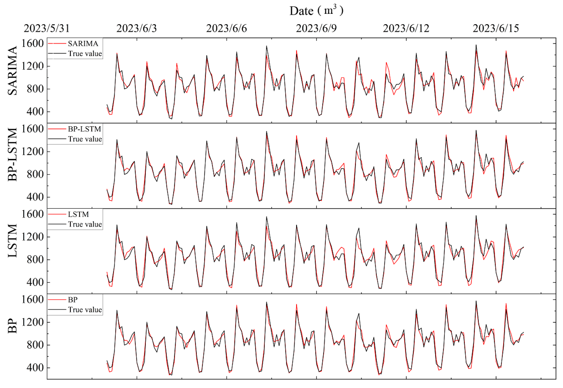
To visually demonstrate the performance of the forecasting models, Figure 9 presents the prediction results of each model on the test dataset. All four models effectively capture the periodic trends in water demand, clearly illustrating the regular 24 h cycle of fluctuations. The predicted values exhibit a high degree of alignment with the actual observations.
However, when faced with periods of frequent changes, such as from 8:00 to 22:00 every day, all models exhibit certain limitations. During this stage, water demand is affected by the interaction of numerous complex dynamic factors, showing drastic and irregular fluctuations. Consequently, the forecasting accuracy of each model declines, and the deviation between predicted and actual values increases markedly.
Notably, the water demand variation pattern from 8:00 to 22:00 on 11 June (Sunday) exhibited a significantly different pattern compared to other dates. Figure 10 illustrates the forecasting performance of the four models from 8:00 to 22:00 on 11 June.
It can be observed that on 11 June, the forecasting performance of the SARIMA model is significantly inferior to that of the other three deep learning models in capturing both the maximum and minimum values. This is because the SARIMA model is a linear model and has higher requirements for the stability of the time series itself, resulting in a significant reduction in its forecasting performance for mutation cases. The single BP and LSTM models show relatively higher or lower forecasting trends compared to other models in predicting the two peaks. The BP-LSTM model outperforms the other three models in both aspects.
To further analyze the performance differences among the models across different time periods, it is necessary to calculate R2, RMSE, and MAPE. These metrics quantify the deviations between predicted values and actual water demand, thereby providing more objective and accurate support for model evaluation and optimization.
As can be seen from Table 5, in terms of the MAPE metric, the errors of the BP-LSTM model are all smaller than those of the other three single forecasting models. Compared with other models, the MAPE is reduced by at least 4.4% and at most 15.8%. Similarly, under the RMSE metric, the BP-LSTM model also exhibits lower error values compared to the other models, with reductions ranging from 2.5% to 16.8%. These results indicate that, in terms of error metrics, the combined forecasting model achieves higher accuracy.
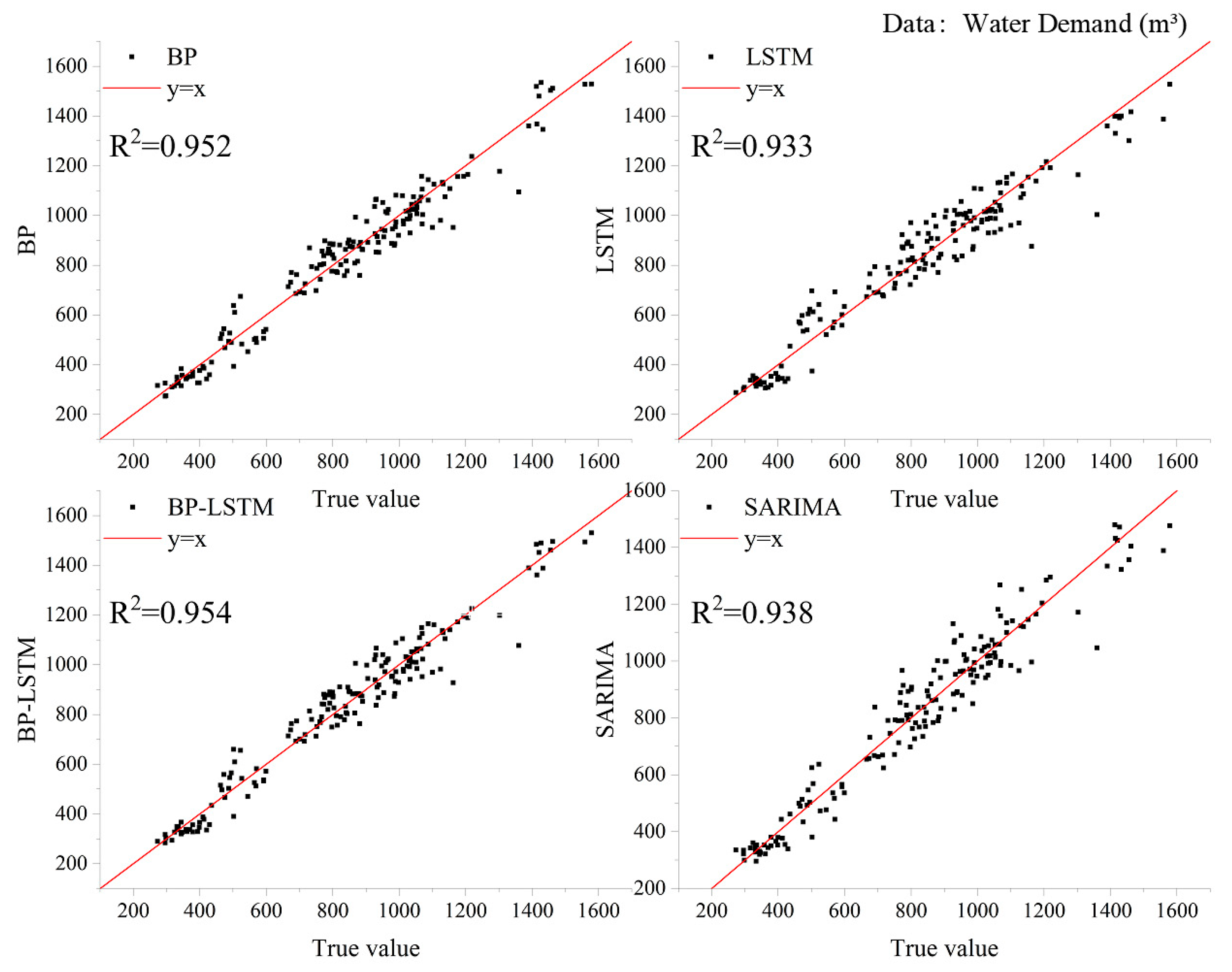
Additionally, Figure 11 presents a comparison between the actual and predicted values of the four model types from a different perspective. The red line represents the ideal case where the predicted values perfectly match the actual values.
From the scatter distribution in the figure, it is evident that the predicted values of all four models are relatively symmetrically distributed around the solid line, with no significant overestimations or underestimations. This balanced distribution helps to minimize cumulative errors in practical applications. Moreover, the R2 values of the four forecasting models are all greater than 0.9. Thus, it can be recognized that the models all have good fitting results. Specifically, the R2 values of the BP and BP-LSTM neural network models are greater than 0.95. This suggests that in time-series forecasting, considering both inherent temporal dependencies and external factors (such as weather and temperature) significantly enhances prediction accuracy.
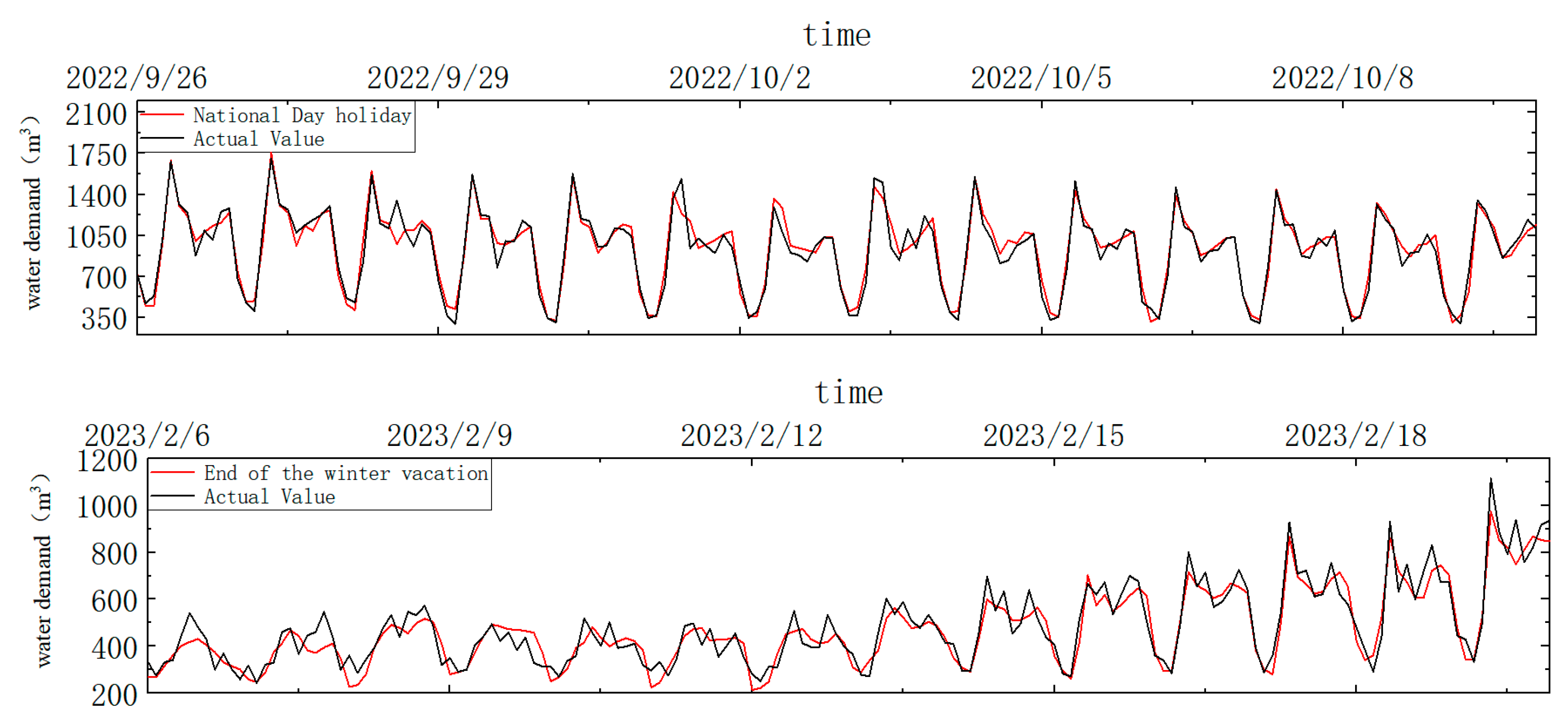
To evaluate the historical fitting and pattern recognition capabilities of the BP-LSTM model in capturing university-specific water demand patterns, a backtesting analysis was conducted. The purpose was to examine whether the model successfully learned and replicated short-term drastic fluctuations in water demand caused by collective student departures and returns within the training data. The backtesting focused on two key periods, the end of the winter break and the National Day holiday, to assess the model’s performance around these distinct seasonal nodes. The National Day holiday occurred from 1 October to 7 October 2022, and the winter break ended on 12 February 2023.
During backtesting, windows consistent with the length of the original test set were selected. Specifically, two-week periods adjacent to both the National Day holiday and the end of the winter break were chosen. The detailed settings are summarized in Table 6.
The backtesting results are presented in Figure 12, which compares predicted and actual values, and Table 7, which summarizes performance metrics.
As shown in Table 7, metrics such as RMSE were significantly better in the backtesting sets compared to the original test set. This improvement can be attributed to the model having learned and memorized historical fluctuation patterns from the training phase. The substantial decrease in RMSE and MAPE, with RMSE reduced by approximately an order of magnitude, indicates a strong ability of the model to reproduce historical holiday water usage patterns within the training data. This reflects successful internalization of water demand patterns, including holiday fluctuations, and demonstrates a high degree of consistency in historical fitting.
The R2 values remained at a relatively high level overall, suggesting that the model consistently captured the major trends in water demand. However, the slight decrease in R2 around the end of the winter break implies that the model’s explanatory power may still be limited under certain scenarios involving abrupt demand changes.
The backtesting evaluation, conducted within the range of the training data, verifies the model’s interpolation performance and its consistency in learning historical patterns. These results indicate that the model has developed a coherent understanding of the underlying data-generating process, thereby laying a foundation for further investigating its extrapolation and generalization capabilities.
To further evaluate the model performance and compare it with existing studies, the evaluation metrics presented in Table 5 were compared with those reported in the relevant literature. A hybrid deep learning model proposed by [17] achieved the best R2 of 0.910 across multiple real-world water use scenarios. In comparison, the BP-LSTM-combined model developed in this study attained an R2 of 0.954, demonstrating superior goodness-of-fit and higher predictive accuracy.
When compared to the DWT-PCA-LSTM model introduced in [27], the proposed model exhibits a comparable level of high accuracy, with an R2 value of 0.954 versus 0.961 reported in [27], indicating that the model presented in this study also offers excellent predictive performance.
In summary, based on comparisons using identical evaluation metrics with existing research, the BP-LSTM combined model proposed in this work demonstrates superior or comparable performance on key indicators, validating the effectiveness of this hybrid approach in enhancing the accuracy of water demand forecasting.

5. Conclusions

This study innovatively proposes a combined BP-LSTM model based on deep learning for water demand forecasting. A comparative analysis was conducted involving traditional single models, such as SARIMA and BP, as well as the emerging single LSTM model. Through a joint FFT and ADF test analysis, the multi-scale periodic characteristics of water demand in high-campus areas were successfully extracted, including a 24 h daily routine cycle, a 7-day teaching cycle, and a 186-day semester cycle. This extraction provides a quantitative basis for selecting model input variables, ultimately aiming to deliver a more accurate forecasting approach for regional water resource planning and management.
The BP-LSTM model integrates the BP neural network and LSTM neural network, effectively combining the strengths of both. It comprehensively accounts for various influencing factors and mitigates the limitations inherent in single models. Consequently, it demonstrates superior forecasting performance compared to the other three models.
The results show that the predicted water demand curves of the four models are close to the actual curve, indicating an overall good fit to the water demand data. Experiments show that for the BP-LSTM model on the test set, the MAPE is 6.48%, which is 15.8%, 4.4%, and 12.6% lower than that of SARIMA, BP, and LSTM, respectively. Similarly, the RMSE of 65.05 is lower by 16.8%, 2.5%, and 13.8%, respectively. The BP-LSTM model, with an R2 value of 0.954, effectively captures the multi-cycle water use patterns of universities. It exhibits superior alignment between predicted and actual values, lower dispersion of deviation, and higher forecasting accuracy. Therefore, the model can be effectively employed to support off-peak scheduling at water plants, thereby reducing energy consumption at pumping stations.
Although this study has achieved meaningful results, opportunities for further improvement remain. Future research could consider additional micro-factors influencing water demand, such as changes in residents’ water usage habits, to further enhance forecasting accuracy. Moreover, advancements in artificial intelligence could inspire more sophisticated model fusion techniques and deeper learning architectures, providing enhanced solutions for water demand forecasting. Finally, comparative studies focusing on water demand forecasting across various regions, examining how water usage patterns differ, and evaluating the applicability of forecasting models under distinct regional characteristics would offer more targeted decision support for broader water resources management.

Author Contributions

Conceptualization, R.Z. and Y.Y.; methodology, R.Z. and H.Y.; software, Y.Y. and H.L.; validation, H.Y. and H.L.; formal analysis, H.Y.; investigation, H.L.; resources, R.Z.; data curation, R.Z.; writing—original draft preparation, H.Y. and Y.Y.; writing—review and editing, H.Y. and R.Z.; visualization, H.Y. and H.L.; supervision, R.Z.; project administration, R.Z.; funding acquisition, R.Z. All authors have read and agreed to the published version of the manuscript.

Funding

This research was funded by the National Natural Science Foundation of China, grant number 52176038.

Data Availability Statement

The original contributions presented in this study are included in the article. Further inquiries can be directed to the corresponding author.

Conflicts of Interest

The authors declare no conflicts of interest.

References

  1. Shah, W.; Chen, J.; Ullah, I.; Shah, M.H.; Ullah, I. Application of RNN-LSTM in Predicting Drought Patterns in Pakistan: A Pathway to Sustainable Water Resource Management. Water 2024, 16, 1492. [Google Scholar] [CrossRef]
  2. Mu, L.; Zheng, F.; Tao, R.; Zhang, Q.; Kapelan, Z. Hourly and Daily Urban Water Demand Predictions Using a Long Short-Term Memory Based Model. J. Water Resour. Plan. Manag. 2020, 146, 05020017. [Google Scholar] [CrossRef]
  3. Howe, C.W.; Linaweaver, F.P. The Impact of Price on Residential Water Demand and Its Relation to System Design and Price Structure. Water Resour. Res. 1967, 3, 13–32. [Google Scholar] [CrossRef]
  4. Miaou, S. A Stepwise Time Series Regression Procedure for Water Demand Model Identification. Water Resour. Res. 1990, 26, 1887–1897. [Google Scholar] [CrossRef]
  5. Xue, X.H.; Xue, X.F.; Xu, L. Study on Improved PCA-SVM Model for Water Demand Prediction. Adv. Mat. Res. 2012, 591–593, 1320–1324. [Google Scholar] [CrossRef]
  6. Zhou, S.; Guo, S.; Du, B.; Huang, S.; Guo, J. A Hybrid Framework for Multivariate Time Series Forecasting of Daily Urban Water Demand Using Attention-Based Convolutional Neural Network and Long Short-Term Memory Network. Sustainability 2022, 14, 11086. [Google Scholar] [CrossRef]
  7. Chen, J.; Boccelli, D.L. Forecasting Hourly Water Demands with Seasonal Autoregressive Models for Real-Time Application. Water Resour. Res. 2018, 54, 879–894. [Google Scholar] [CrossRef]
  8. Chen, G.; Long, T.; Xiong, J.; Bai, Y. Multiple Random Forests Modelling for Urban Water Consumption Forecasting. Water Resour. Manag. 2017, 31, 4715–4729. [Google Scholar] [CrossRef]
  9. Iwakin, O.; Moazeni, F. Improving Urban Water Demand Forecast Using Conformal Prediction-Based Hybrid Machine Learning Models. J. Water Process Eng. 2024, 58, 104721. [Google Scholar] [CrossRef]
  10. Fu, G.; Jin, Y.; Sun, S.; Yuan, Z.; Butler, D. The Role of Deep Learning in Urban Water Management: A Critical Review. Water Res. 2022, 223, 118973. [Google Scholar] [CrossRef] [PubMed]
  11. Donkor, E.A.; Mazzuchi, T.A.; Soyer, R.; Roberson, J.A. Urban Water Demand Forecasting: Review of Methods and Models. J. Water Resour. Plan. Manag. 2014, 140, 146–159. [Google Scholar] [CrossRef]
  12. Liu, X.; Sang, X.; Chang, J.; Zheng, Y. Multi-Model Coupling Water Demand Prediction Optimization Method for Megacities Based on Time Series Decomposition. Water Resour. Manag. 2021, 35, 4021–4041. [Google Scholar] [CrossRef]
  13. Wang, T. Zhenjiang June 2022 Historical Weather. 2022. Available online: https://lishi.tianqi.com/zhenjiang/202206.html (accessed on 20 August 2025).
  14. China Meteorological Administration. Official Website. Available online: https://www.cma.gov.cn/ (accessed on 20 August 2025).
  15. Huang, H.; Zhang, Z.; Song, F. An Ensemble-Learning-Based Method for Short-Term Water Demand Forecasting. Water Resour. Manag. 2021, 35, 1757–1773. [Google Scholar] [CrossRef]
  16. Ghiassi, M.; Zimbra, D.K.; Saidane, H. Urban Water Demand Forecasting with a Dynamic Artificial Neural Network Model. J. Water Resour. Plan. Manag. 2008, 134, 138–146. [Google Scholar] [CrossRef]
  17. Wang, K.; Xie, X.; Liu, B.; Yu, J.; Wang, Z. Reliable Multi-Horizon Water Demand Forecasting Model: A Temporal Deep Learning Approach. Sustain. Cities Soc. 2024, 112, 105595. [Google Scholar] [CrossRef]
  18. Szostek, K.; Mazur, D.; Drałus, G.; Kusznier, J. Analysis of the Effectiveness of ARIMA, SARIMA, and SVR Models in Time Series Forecasting: A Case Study of Wind Farm Energy Production. Energies 2024, 17, 4803. [Google Scholar] [CrossRef]
  19. Guo, G.; Liu, S.; Wu, Y.; Li, J.; Zhou, R.; Zhu, X. Short-Term Water Demand Forecast Based on Deep Learning Method. J. Water Resour. Plan. Manag. 2018, 144, 04018076. [Google Scholar] [CrossRef]
  20. Wang, Y.; Qin, L.; Wang, Q.; Chen, Y.; Yang, Q.; Xing, L.; Ba, S. A Novel Deep Learning Carbon Price Short-Term Prediction Model with Dual-Stage Attention Mechanism. Appl. Energy 2023, 347, 121380. [Google Scholar] [CrossRef]
  21. Almanjahie, I.M.; Chikr-Elmezouar, Z.; Bachir, A. Modeling and Forecasting the Household Water Consumption in Saudi Arabia. Appl. Ecol. Environ. Res. 2019, 17, 1299–1309. [Google Scholar] [CrossRef]
  22. Tian, Y.; Wu, Q.; Zhang, Y. A Convolutional Long Short-Term Memory Neural Network Based Prediction Model. Int. J. Comput. Commun. Control 2020, 15, 3906. [Google Scholar] [CrossRef]
  23. Wu, J.; Wang, Z.; Dong, L. Prediction and Analysis of Water Resources Demand in Taiyuan City Based on Principal Component Analysis and BP Neural Network. J. Water Supply Res. Technol.-Aqua 2021, 70, 1272–1286. [Google Scholar] [CrossRef]
  24. Tang, Z.Q.; Liu, G.; Xu, W.N.; Xia, Z.Y.; Xiao, H. Water Demand Forecasting in Hubei Province with BP Neural Network Model. Adv. Mat. Res. 2012, 599, 701–704. [Google Scholar] [CrossRef]
  25. Zou, S.; Ren, X.; Wang, C.; Wei, J. Impacts of Temporal Resolution and Spatial Information on Neural-Network-Based PM2.5 Prediction Model. Acta Sci. Nat. Univ. Pekin. 2020, 56, 417–426. [Google Scholar]
  26. Kavya, M.; Mathew, A.; Shekar, P.R.; Sarwesh, P. Short Term Water Demand Forecast Modelling Using Artificial Intelligence for Smart Water Management. Sustain. Cities Soc. 2023, 95, 104610. [Google Scholar] [CrossRef]
  27. Du, B.; Zhou, Q.; Guo, J.; Guo, S.; Wang, L. Deep Learning with Long Short-Term Memory Neural Networks Combining Wavelet Transform and Principal Component Analysis for Daily Urban Water Demand Forecasting. Expert. Syst. Appl. 2021, 171, 114571. [Google Scholar] [CrossRef]
  28. Hu, P.; Tong, J.; Wang, J.; Yang, Y.; Oliveira Turci, L. de A Hybrid Model Based on CNN and Bi-LSTM for Urban Water Demand Prediction. In Proceedings of the 2019 IEEE Congress on Evolutionary Computation (CEC), Wellington, New Zealand, 10–13 June 2019; IEEE: New York, NY, USA; pp. 1088–1094. [Google Scholar]
  29. Cao, K.; Kim, H.; Hwang, C.; Jung, H. CNN-LSTM Coupled Model for Prediction of Waterworks Operation Data. J. Inf. Process. Syst. 2018, 14, 1508–1520. [Google Scholar] [CrossRef]
  30. Hu, S.; Gao, J.; Zhong, D.; Deng, L.; Ou, C.; Xin, P. An Innovative Hourly Water Demand Forecasting Preprocessing Framework with Local Outlier Correction and Adaptive Decomposition Techniques. Water 2021, 13, 582. [Google Scholar] [CrossRef]
  31. Xenochristou, M.; Kapelan, Z. An Ensemble Stacked Model with Bias Correction for Improved Water Demand Forecasting. Urban Water J. 2020, 17, 212–223. [Google Scholar] [CrossRef]
  32. Stańczyk, J.; Kajewska-Szkudlarek, J.; Lipiński, P.; Rychlikowski, P. Improving Short-Term Water Demand Forecasting Using Evolutionary Algorithms. Sci. Rep. 2022, 12, 13522. [Google Scholar] [CrossRef]
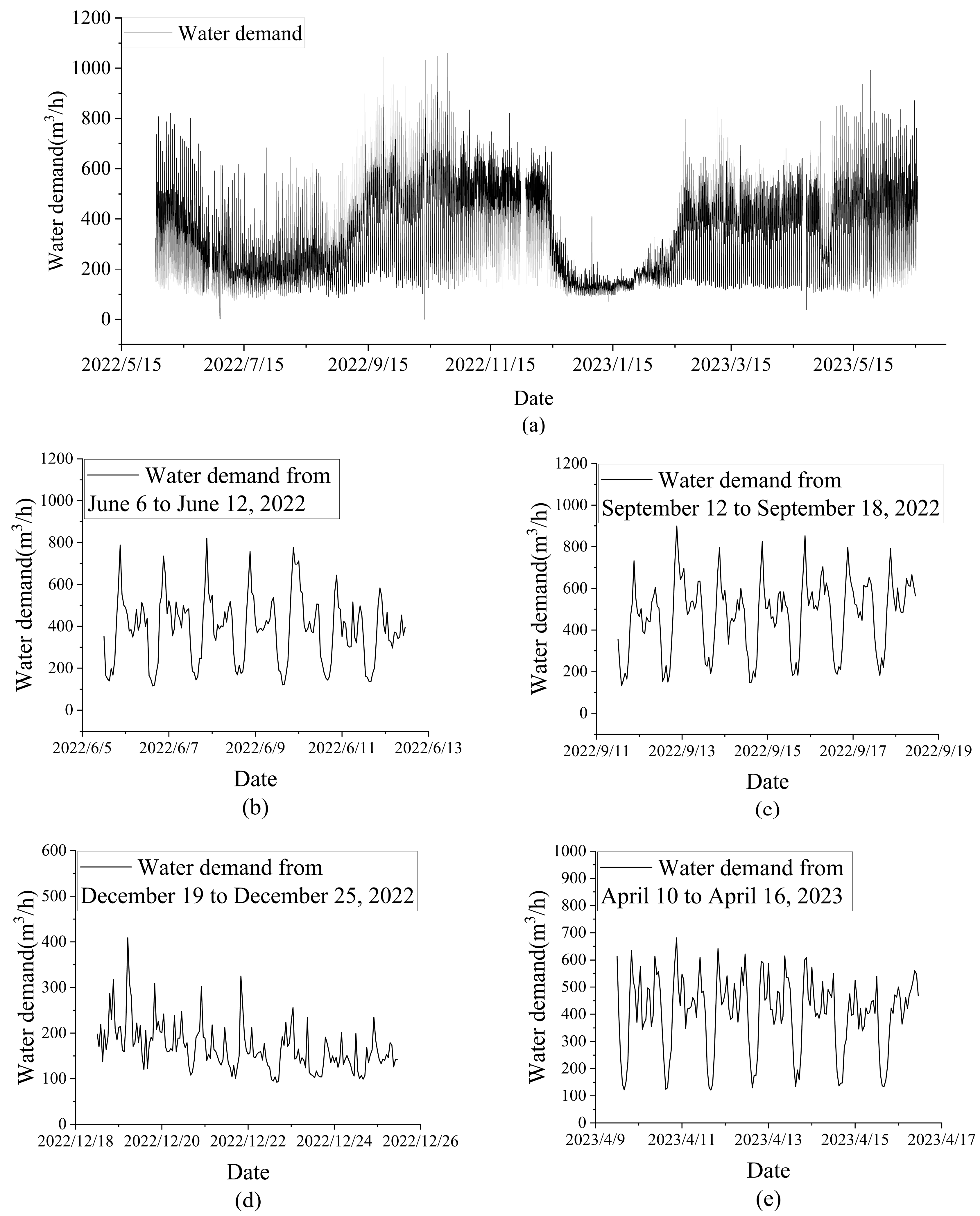
Figure 1. Water demand changes from 1 June 2022 to 15 June 2023: (a) Overview; (be) Data of one week randomly selected.
Water 17 02729 g001
Figure 2. Example of missing data imputation.
Water 17 02729 g002
Figure 3. Example of abnormal data modification.
Water 17 02729 g003
Figure 4. Frequency-amplitude plot of water demand data after fast Fourier transform.
Water 17 02729 g004
Figure 5. First and second order difference results of raw water demand data.
Water 17 02729 g005
Figure 6. Autocorrelation coefficient of the original data after first differencing.
Water 17 02729 g006
Figure 7. The overall structure and data direction of the combined model.
Water 17 02729 g007
Figure 8. LSTM model structure.
Water 17 02729 g008
Figure 9. Forecasting from different models.
Water 17 02729 g009
Figure 10. Forecasting performance of four water demand forecasting models from 8 to 22 on 11 June.
Water 17 02729 g010
Figure 11. Comparison of the predicted values and real values of different models.
Water 17 02729 g011
Figure 12. Comparison of backtesting predicted and actual values.
Water 17 02729 g012
Table 1. Points A to E correspond to the time period case.
ABCDE
Period186 days7 days24 h12 h8 h
Table 2. ADF test results.
T-Valuep-ValueStatistical Values for Varying Degrees of Rejection of the Null Hypothesis
1%5%10%
Raw date−1.920.32−3.43−2.86−2.57
First-order difference−19.560−3.43−2.86−2.57
Second-order difference−25.890−3.43−2.86−2.57
Table 3. BP neural network input example.
NameValueNameValue
The data of the previous week1283Month6
The data of the previous day1272Date8
The data of the previous hour450Day of week5
Hours of day3
Data of the previous 12 h501Maximum temperature31
Wind speed3Minimum temperature18
Table 4. BP, LSTM, and BP-LSTM neural network model hyperparameters.
Number of
Hidden Layers
The Number of Neurons in Each Hidden LayerLearning RateBatch Size
BP neural network3(64, 64, 16)2.5 × 10−464
LSTM neural network2(128, 128)10−432
BP-LSTM neural network2(16, 8)10−532
Table 5. Evaluation and comparison of four forecasting model indicators.
SARIMABPLSTMBP-LSTM
R20.9380.9520.9330.954
RMSE (m3)75.5066.7178.1865.05
MAPE7.41%6.78%7.70%6.48%
Table 6. Backtesting periods and data volume.
Backtesting IntervalNumber of Data Points
National Day26 September to 9 October 2022168
Winter Break End6 February to 19 February 2023168
Table 7. Backtesting performance metrics.
R2RMSE (m3)MAPE
National Day0.9396.842.77
Winter Break End0.8801.275.91
Disclaimer/Publisher’s Note: The statements, opinions and data contained in all publications are solely those of the individual author(s) and contributor(s) and not of MDPI and/or the editor(s). MDPI and/or the editor(s) disclaim responsibility for any injury to people or property resulting from any ideas, methods, instructions or products referred to in the content.