Article

Runoff Forecast Model Integrating Time Series Decomposition and Deep Learning for the Short Term: A Case Study in the Weihe River Basin, China

1
State Key Laboratory of Efficient Utilization of Agricultural Water Resources, China Agricultural University, Beijing 100083, China
2
Center for Agricultural Water Research in China, China Agricultural University, Beijing 100083, China
3
College of Water Resources and Civil Engineering, China Agricultural University, Beijing 100083, China
4
Key Laboratory of Water Cycle and Related Land Surface Processes, Institute of Geographic Sciences and Natural Resources Research, Chinese Academy of Sciences, Beijing 100101, China
5
University of Chinese Academy of Sciences, Beijing 100190, China
*
Author to whom correspondence should be addressed.
Water 2025, 17(18), 2718; https://doi.org/10.3390/w17182718
Submission received: 31 July 2025 / Revised: 7 September 2025 / Accepted: 12 September 2025 / Published: 14 September 2025

Abstract

Accurate prediction of river runoff is significant for flood control, water resource allocation, and basin ecological management. Despite the promise of integrating signal decomposition with deep learning, current decomposition-based hybrid models face critical forward data contamination: decomposition algorithms improperly access future test data in full-series applications, artificially inflating prediction accuracy. In contrast, the stepwise decomposition method currently proposed leads to high computational costs. To address this limitation, we introduce a novel framework integrating segmented decomposition sampling with a multi-input neural network. Specifically, a hybrid forecasting model combining Seasonal-Trend decomposition using Loess (STL) and Convolutional Long Short-Term Memory (CNN-LSTM) networks was implemented for daily runoff estimation. Method reliability was evaluated using historical runoff data from Huaxian Station in China’s Weihe River Basin, with comparative experiments conducted against established single and hybrid models. The results showed that the proposed framework can effectively avoid future information leakage and simultaneously improve prediction accuracy. For 1–3-day-ahead Nash-Sutcliffe efficiency (NSE) at Huaxian Station, the STL-CNN-LSTM model achieved values of 0.96, 0.83, and 0.80, respectively—representing improvements of 5.49%, 5.06%, and 12.68% over the VMD-CNN-LSTM model. This STL-based configuration outperformed the standalone LSTM counterpart by 23.08%, 9.21%, and 17.65% in NSE, respectively. Therefore, the proposed framework, which incorporates the segmented decomposition sampling method and a multi-input neural network, proves to be both practical and reliable.

1. Introduction

As a pivotal element of hydrological forecasting systems, runoff prediction constitutes a core research focus [1]. Accurate short-term runoff prediction and the identification of key driving factors are essential for the rational allocation of water resources [2,3]. While long-term projections are valuable for planning, the short-term forecast horizon presents a distinct challenge due to the need to capture rapidly evolving atmospheric and hydrological processes [4]. Current runoff prediction models primarily fall into two categories: physically based hydrological models and data-driven models [5,6]. Physically based models effectively simulate hydrological processes, but their predictive accuracy is substantially degraded when forecast lead times exceed the critical duration required for runoff concentration within the watershed [7]. The complexity of rainfall-runoff processes at the watershed scale has been further exacerbated by synergistic effects of climatic variability, underlying surface alterations, and anthropogenic activities [8]. In contrast, data-driven models do not require a clear understanding of the specific hydrological mechanisms of a watershed; instead, they can directly uncover the nonlinear relationships between input factors and runoff from a data perspective [9,10].
Data-driven approaches to runoff prediction primarily encompass time series analysis models and machine learning techniques, both extensively developed and applied in hydrological forecasting [11]. Traditional time series models, such as autoregressive (AR) models and autoregressive integrated moving average (ARIMA) models, have played a crucial role in runoff forecasting analysis [12,13,14]. Nevertheless, owing to the multifaceted complexity characterizing hydrological processes, these models, which are based on linear assumptions, are not sufficient to fully mine all the features of the data and are not suitable for predicting the non-stationary runoff series [15,16]. Recent advancements in computer technology and artificial intelligence, especially those represented by artificial neural networks, have significantly transformed the methods of forecasting [17,18,19,20]. These methods can be used to extract key features from data and effectively handle complex nonlinear relationships and interactions between multiple variables [21,22]. Additionally, they are capable of accurately capturing the temporal and spatial structural characteristics of hydrological, meteorological, and geographical data [23].
While machine learning models excel at fitting complex relationships, a single machine learning model often struggles to fully capture the intricate periodicity, transient behaviors, and trend information present in runoff time series [24,25], especially in daily runoff prediction [26]. This difficulty is compounded by the inherent non-stationarity and noise components frequently found in runoff data, which can obscure underlying patterns and degrade model performance [27]. Developing a hybrid forecasting model based on decomposition is seen as an effective approach to enhancing runoff prediction accuracy [28]. Fundamentally, this approach decomposes original runoff series into constituent components to capture intrinsic variation patterns, resulting in improved forecasting precision [1,10]. Decomposition yields multiscale features that are inherently simpler and more regular than the original composite signal. Modeling these decomposed components enables machine learning techniques to more effectively characterize the underlying dynamics and leverage the information embedded within each component, thereby enhancing predictive accuracy [29].
Runoff sequence decomposition techniques can primarily be categorized into two types: time series decomposition and time-frequency signal decomposition methods. The former method centers on extracting key data features such as trends, seasonal patterns, and periodic components. This method proves particularly useful when dealing with intricate time-dependent data, aiding in both analysis and prediction. The main methods are, for example, Breaks For Additive Season and Trend (BFAST) [30], Seasonal Extraction in ARIMA Time Series (SEATS) [31], and Seasonal-Trend decomposition using Loess (STL) [32]. STL stands out for its robustness against outliers and versatility in handling various seasonality types, making it promising for runoff prediction across scales [33]. The predominant time-frequency methods are Discrete Wavelet Transform (DWT) [34], Empirical Mode Decomposition (EMD) [35], and Variational Mode Decomposition (VMD) [2]. VMD is valuable for preprocessing time series by breaking down complex signals into simpler, more manageable sub-signals for machine learning modeling [35]. Decomposition methods have a direct impact on hybrid runoff forecasting model performance. Currently, while both methods have been applied to runoff forecasting, studies that empirically and systematically compare their relative performance are notably lacking. Zhang et al. (2005) contend that the complex multi-scale periodicity of runoff series fundamentally compromises modeling accuracy when decomposition techniques like VMD neglect explicit seasonal component extraction [36]. Incorporating inherent seasonal components is critical for accurate runoff modeling. And the comparative evaluation of different main decomposition methods is important for building a decomposition-based hybrid forecasting framework.
A critical flaw in many decomposition-based models for runoff forecasting is the artificially inflated accuracy caused by information leakage. This well-documented issue arises from applying decomposition holistically to the entire time series, which inadvertently incorporates future data into the model’s explanatory variables [37,38,39]. In essence, models trained on such data exhibit spuriously high performance on test samples by implicitly leveraging future information during training. Thus, overall sampling remains hydrologically implausible, and falsely high predictive performance is not credible [14]. Although stepwise decomposition frameworks effectively eliminate this leakage through iterative processing [14,33], they impose prohibitively high computational costs. To address these critical limitations, this study introduced an innovative segmented decomposition framework employing decomposition methods with a unit sliding constant increment mechanism. This temporally constrained strategy ensures that each decomposition step utilizes only contemporaneous and historical hydrological data, thereby rigorously preventing future information leakage. While this rigorous decomposition might theoretically lead to a degradation in prediction performance compared to traditional decomposition methods, it ensured that the predictions are physically valid [27,40,41].
The key contributions of this study are as follows: To explore the practical and effective application of time series decomposition in runoff prediction, we developed a segmented decomposition framework that strictly precludes the use of any future information. Building upon this architecture, we further proposed an innovative hybrid model that integrates STL with CNN-LSTM techniques for runoff forecasting. The validity and advantages of our proposed framework were demonstrated through three-day-ahead runoff forecasting experiments conducted at Huaxian Station in the Weihe River Basin, China.

2. Materials and Methods

2.1. Study Area and Data

As a major tributary of the Yellow River, the Weihe River was selected as the study area. The Weihe River originates in Weiyuan County, Gansu Province, and converges with the Yellow River in Tongguan County, Shaanxi Province [42]. The river’s topography is characterized by high elevations in the surrounding areas and lower elevations in the central region. The Weihe River Basin is characterized by a temperate monsoon climate with an average annual temperature of 12–14 °C and mean annual precipitation ranging from 500 to 700 mm. The precipitation exhibits significant seasonal and inter-annual variability, with over 60% of the annual total occurring during the wet season (July to September), leading to frequent spring droughts and summer floods [43]. As illustrated in Figure 1, it is located between longitudes 103°5′ E and 110°5′ E, and latitudes 33°5′ N and 37°5′ N. The main channel of the Weihe River spans a total length of 818 km, with a drainage area of 134,800 square kilometers [44]. As illustrated in Table 1, this study used daily runoff measurements from the Huaxian Station, located on the lower Weihe River, for the period 1990–2019 to validate the predictive performance of the proposed forecasting framework and model.
The expanded integration of remote sensing data enhances runoff simulation capabilities by providing high-resolution spatial heterogeneity information [45]. Building on this capability, we incorporated the following remote sensing data as model inputs to further improve prediction accuracy. Meteorological data, including precipitation, air temperature, surface pressure, specific humidity, downward longwave radiation, and downward shortwave radiation, were sourced from the China Meteorological Forcing Dataset (CMFD) (National Tibetan Plateau Data Center, Chinese Academy of Sciences, Beijing, China). This dataset has a spatial resolution of 0.1° × 0.1° and covers the period from 1990 to 2019 [46,47]. Additionally, the Normalized Difference Vegetation Index (NDVI) dataset were obtained from the MOD13C2 product (LP DAAC, USGS, Sioux Falls, SD, USA). This dataset possesses a spatial resolution of 0.05° × 0.05° and spans the duration from 2000 to 2019. The hydrological information data center of the Shaanxi Hydrographic and Water Resources Survey Bureau (Xi‘an, China) provided the streamflow records. Daily runoff records (1990–2019) for key mainstream stations in the Weihe River Basin were obtained from the Annual hydrological report, P. R. China (Ministry of Water Resources, Beijing, China).

2.2. Methodologies

2.2.1. Runoff Sequence Decomposition Methods

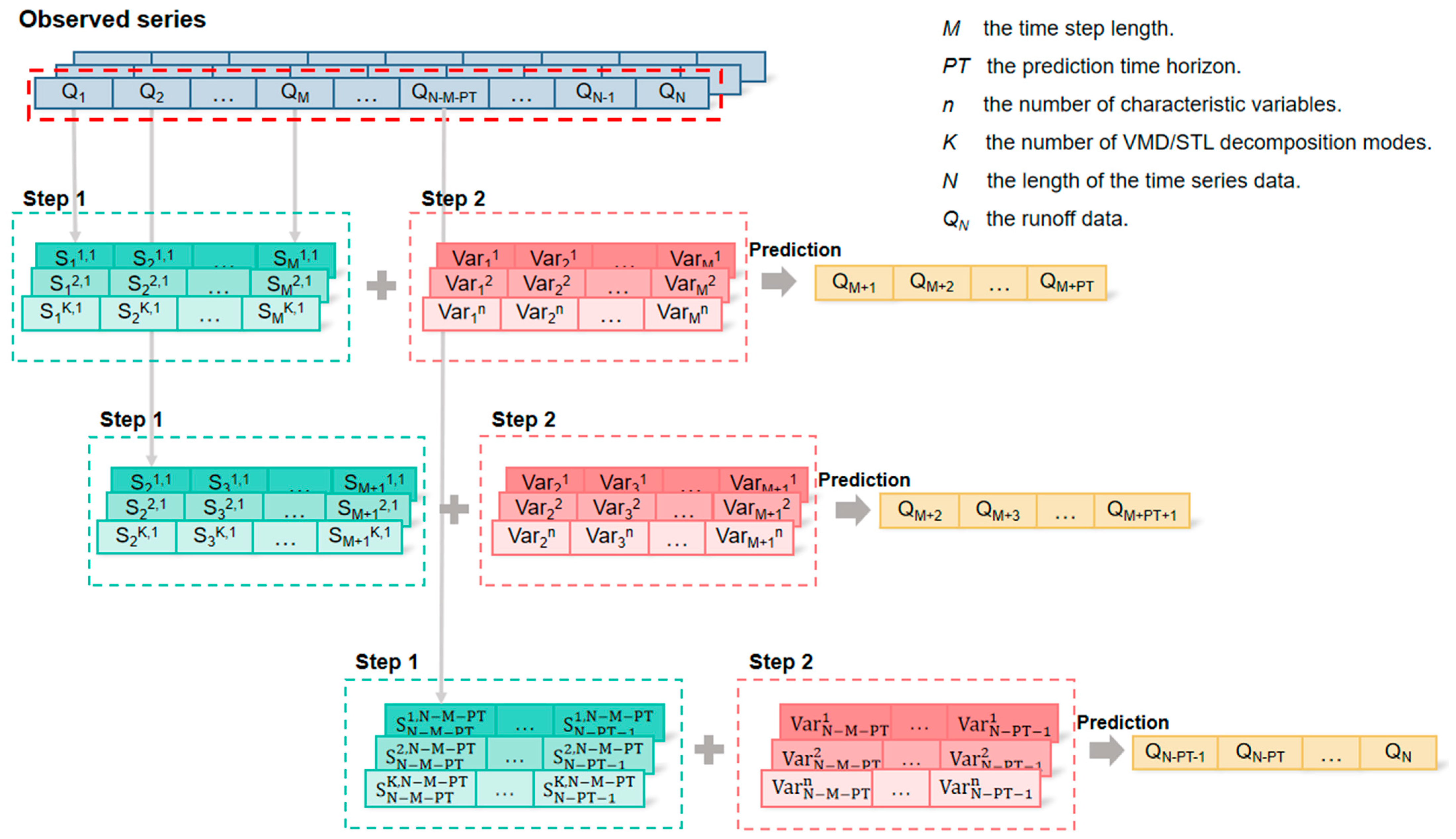
Many existing studies have opted for overall decomposition before prediction, which can lead to information leakage and inflate prediction accuracy [37,38,39]. As schematically illustrated in Figure 2, our segmented decomposition-based sampling technique rigorously adhered to temporal causality through a constant increment mechanism. The implementation comprised three operational phases: The first decomposition window spanned historical runoff observations from Q 1 (the first runoff observation in the sequence) to Q M (the M-th observation in the sequence), where M denotes the required antecedent period for hydrological memory effects. The decomposition methods were applied exclusively to this initial sequence to derive decomposed sequences, from which predictive features for forecasting Q 1 to Q M were extracted. Secondly, upon acquiring the observed Q 2 value, the window advanced by one timestep, incorporating the new observation while discarding the oldest data point. The decomposition methods were reinitialized on the updated sequence [ Q 2 , …, Q N M P T ], where PT represents the prediction time horizon. Transient hydrological features from the fresh decomposition informed predictors for Q N M P T . This causal decomposition-prediction cycle persisted until reaching the current timestep Q N M P T , with each iteration: maintaining a fixed window length (M) through forward sliding. The decomposition continued stepwise until all model training and test samples were available. Response variables across all model samples were preserved as undecomposed observations sourced exclusively from the initial runoff sequence, without utilizing decomposed elements. The runoff decomposition volume is shown in Step 1. The other variables in Step 2 are the aforementioned meteorological and subsurface data, which are temporally aligned with the data used in Step 1. For this study, M is set to 40 days through Partial Autocorrelation Function (PACF) analysis (see Section 2.2.3 for details), PT to 3, and n to 37 (where n is the number of characteristic variables).
Variational Mode Decomposition
Dragomiretskiy and Zosso proposed the VMD method [48] in 2014, which is a time-frequency signal decomposition method. VMD is a data decomposition technique that determines optimal solutions for variational models through iterative computation. VMD decomposes a complex time series into multiple Intrinsic Mode Functions (IMFs) with different time scales and residual components. Each IMF represents a specific oscillation or trend, which efficiently captures the potential modal effects of the time series at different time scales. This method adapts to data’s intrinsic characteristics, proving particularly effective for analyzing complex non-stationary sequences like daily runoff. The input signal f ( t ) is formally defined by the following variational model:
m i n u k , w k { k = 1 K t δ t + j π t     u k t e j ω k t 2 2 } s . t .   k = 1 K u k t = f t
where K is the number of subsequence IMFs, u k = { u 1 , u 2 , , u k } is the set of all IMFs, ω k = { ω 1 , ω 2 , , ω k } is the corresponding center frequency of each IMF, δ t is the impulse function, and * is the convolution operator.
Seasonal-Trend Decomposition Procedures Based on Loess
STL is a time series decomposition method based on locally weighted regression (Loess) [49], which smooths the time series through locally weighted regression, and the iterative process decomposes the Trend, Seasonal, and Remainder of the time series. The STL method has the advantages of strong flexibility, wide range of application, and the ability to deal with nonlinear and irregular data, and it is often used in meteorology, hydrology, and other fields of time series analysis. Its basic formula is:
Y t = T t + S t + R t
where Y t is the observed value of the time series; T t is the trend component; S t is the seasonality component; R t is the residual component.
Among various techniques for breaking down time series data, STL stands out chiefly because of its exceptional ability for outliers in the time series. This capability enables decomposition into stable component subsequences, consequently elevating model forecasting precision and enhancing prediction accuracy [33].

2.2.2. Light Gradient Boosting Machine

The Light Gradient Boosting Machine (LightGBM) is an implementation of a tree-based ensemble method called gradient boosting. This method makes predictions sequentially, combining weak predictive tree models and learning from their mistakes [33]. In this study, the selection of characteristic variables was performed by accumulating the importance of each variable by LightGBM. The top 20 variables were selected based on their importance and used as input factors for constructing the runoff prediction model.

2.2.3. Partial Autocorrelation Function

The Partial Autocorrelation Function (PACF) determines direct relationships in time series while controlling for other variables’ effects. Time steps critically impact model performance: although LSTM networks utilize gating mechanisms to capture long-term dependencies, an excessively long time step may introduce noise accumulation, while an insufficient step length risks omitting critical temporal trends [50]. The PACF has been extensively employed as a well-established methodology for identifying optimal time step lengths in time series modeling [51,52]. The LSTM model efficiently removes unnecessary data, enabling the selection of a larger time step for runoff prediction [33]. Given computational constraints and LSTM characteristics, this study uses a 40-day sequence of preceding daily runoff values as model inputs.

2.2.4. Integrated CNN-LSTM Forecasting Model

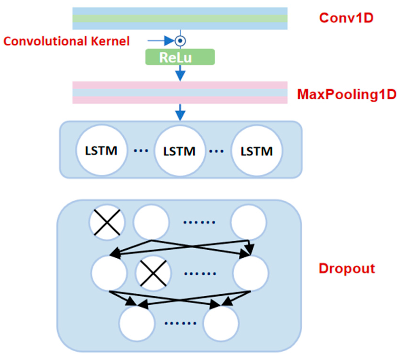
The CNN-LSTM model outperformed the LSTM model in identifying complex feature representations by stacking several convolutional and pooling layers [53]. The CNN-LSTM model integrates two parts: the CNN part, which includes convolutional and max pooling layers, and the LSTM part. The CNN uses convolutional kernels to extract deep nonlinear features hidden in the data. Through convolutional operations, the initial feature matrix generated in convolutional layers exhibits superior representational capacity compared to original time series [54]. The convolutional layers utilize Rectified Linear Unit (ReLU) activation functions to introduce nonlinearity into the model. Subsequent maximum pooling layers further enhance feature expressiveness by processing the convolutional output. Collectively, the CNN component functions as an advanced data processing structure, delivering refined sequences to the LSTM part for enhanced temporal pattern recognition. The LSTM part excels in learning sequential dependencies and maintaining short-term memory, effectively capturing latent temporal dynamics in the data streams. Integrating CNN and LSTM combines the strengths of both architectures. Figure 3 illustrates the integrated CNN-LSTM architecture.

2.2.5. Decomposition Ensemble Models for Runoff Forecasting

Decomposition-ensemble forecasting models face a critical issue: information leakage artificially inflates prediction performance. To mitigate this issue while practically enhancing runoff forecasting accuracy, we developed a segmented decomposition sampling with a multi-input neural network framework and established the STL-CNN-LSTM runoff forecasting model (as illustrated in Figure 4): (i) Segmented decompositions were executed on fixed runoff sequences (M-40 days) using strict forward-propagation, ensuring each decomposition cycle incorporated only antecedent observations prior to prediction targets. (ii) Gridded climate data were integrated with in situ hydrometeorological observations, and predictors exhibiting dominant influence were extracted as model inputs. (iii) The Sparrow Search Algorithm (SSA) optimized model parameters, while a multi-input CNN-LSTM architecture extracted spatiotemporal features to simulate predictor-runoff relationships, ultimately generating runoff forecasts.
The implementation of the proposed runoff forecasting framework integrates data preprocessing, decomposition, and hybrid modeling. First, the LightGBM selects input variables based on cumulative feature importance (top 70%), while decomposition parameters—such as K and α for VMD and the periodicity for STL—are optimized using Bayesian optimization with Gaussian processes. The original runoff sequence is partitioned into units ( Q 1 to Q M ), which are decomposed using both VMD and STL methods. Spatiotemporal driving factors from the Weihe Basin are incorporated, and subsequent segments ( Q 2 to Q N M P T ) are iteratively decomposed to construct training samples, with Q M + 1 to Q M + P T as prediction targets. The samples are split into calibration and validation sets in a 4:1 ratio based on chronological year. A multi-input CNN-LSTM model is employed to extract spatiotemporal features, trained on the calibration set and further optimized using the SSA. Predictions are generated from the validation set inputs and evaluated using standard performance metrics.

2.2.6. Performance Assessment

The predictive performance of the model on the test set was quantitatively characterized by Nash-Sutcliffe Efficiency (NSE), Root Mean Square Error (RMSE), and Mean Absolute Error (MAE).
N S E = 1 i = 1 n y 0 i y c i 2 i = 1 n y 0 i y 0 ¯ 2
R M S E = 1 n i = 1 n y 0 i y c i 2
M A E = i = 1 n y 0 i y c i
where y 0 i is the measured value at time i ; y c i is the predicted value at time i ; y 0 ¯ is the mean of predicted values; and n is the length of the data series.

3. Results

3.1. Comparative Analysis of CNN-LSTM and Standalone LSTM Performance

Among the data-driven runoff models, those based on the LSTM network showed good performance. Based on the hydrometeorological dataset described in Section 2.1 (daily records at 19 monitoring stations) and the evaluation metrics outlined in Section 2.2.6, we constructed an LSTM model based on the optimization of the SSA for daily runoff prediction. As demonstrated in Table 2, the LSTM model achieved competent performance. However, an analysis of its performance revealed a marked increase in MAE (from 37.47 m3/s to 56.18 m3/s) and RMSE (from 101.06 m3/s to 120.56 m3/s) as the forecast horizon extended from day 1 to day 3. This significant performance degradation highlighted the limitations of the standard LSTM in capturing features, necessitating a more sophisticated architecture. To address this degradation in accuracy, we introduced a CNN component to form a hybrid model. The CNN-LSTM combines the local feature extraction capability of CNN with the time-series modeling capability of LSTM to achieve accurate modeling of complex hydrological processes. As shown in Table 2, the hybrid model improved the overall accuracy compared to the standalone LSTM, demonstrating its superiority.
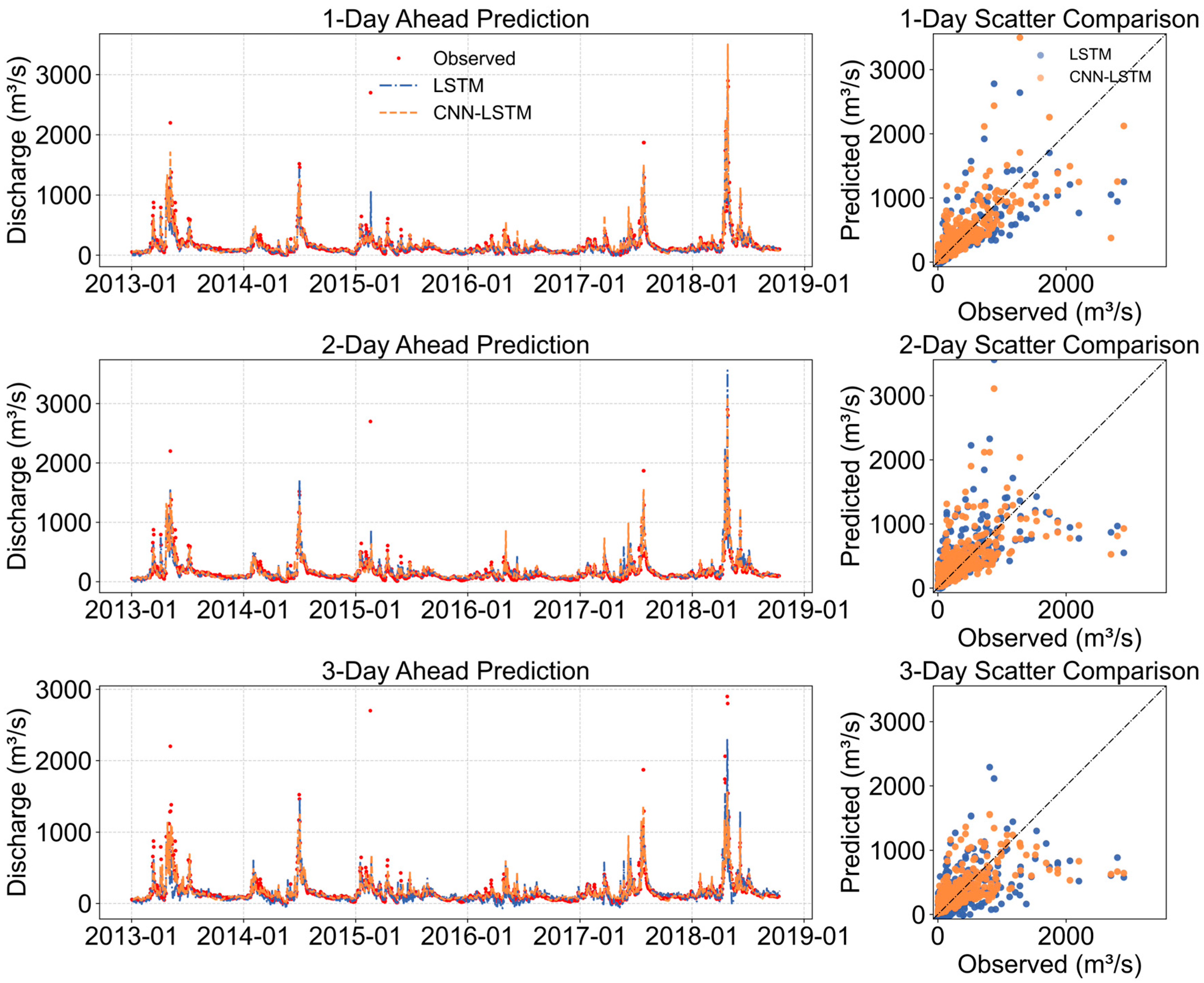
The integration of a CNN layer for enhanced feature extraction significantly improved the model prediction ability. Overall, the CNN-LSTM model achieved higher prediction accuracy in runoff forecasting at Huaxian Station compared to the standalone LSTM model. Specifically, the RMSE of the CNN-LSTM model drops by 8.81% on the first day, 6.54% on the second day, and 2.23% on the third day compared to the standard LSTM approach. The NSE accuracy gains of 4.79%, 3.69%, and 2.12% were observed for one-, two-, and three-day forecasts, respectively, in comparison to using only LSTM. However, the CNN-LSTM model exhibited an increase in the MAE of 10.67% on day 1 and 1.69% on day 2, while achieving a substantial reduction of 11.50% on day 3 compared to the LSTM baseline. This pattern suggests that the standalone LSTM model achieved stable predictions under most conditions (resulting in lower MAE) but produced substantially larger errors at critical points, such as flow peaks. In contrast, although the CNN-LSTM model introduced slightly higher average errors in some cases (contributing to its increased MAE on days 1 and 2), it was more effective at mitigating extreme prediction inaccuracies. To visually evaluate the accuracy of different methods, Figure 5 presents a comparison between forecasted and observed runoff from the validation set using both the LSTM and CNN-LSTM models. The predictions generated by the CNN-LSTM model more closely follow the observed runoff dynamics at Huaxian Station, capturing hydrograph variations with greater fidelity. Across most evaluation metrics, the CNN-LSTM model exhibits superior performance compared to the standalone LSTM, although the degree of improvement decreases as the forecast horizon lengthens. This indicates that CNN-based feature extraction enhances the model’s short-term predictive ability, whereas long-term forecasting remains a persistent challenge. To further improve the prediction of peak flow events, decomposition methods were incorporated into the modeling framework to isolate extreme hydrological patterns, thereby increasing predictive robustness.

3.2. Comparative Analysis of VMD and STL Decomposition Performance

To enhance forecasting accuracy while preventing information leakage, this study incorporated a segmented decomposition strategy into the prediction framework. Given the demonstrated efficacy and wide adoption of both STL and VMD, these methods were selected for representative comparison. Each was integrated with a CNN-LSTM runoff prediction model to leverage its capability in effectively extracting spatial features from the input data. In this study, the Bayesian optimization was applied to optimize the parameters of VMD and STL. Through this process, the optimal parameter combination of VMD was determined to be K was determined to be 10, and the penalty factor α was determined to be 500. Concurrently, the optimal parameter combination of STL was determined, with the seasonal length set to 11 and the trend window length set to 413.
As quantified in Table 3, the VMD-CNN-LSTM model outperformed the CNN-LSTM model across all lead times. For one-day-ahead predictions, both the MAE and RMSE decreased significantly, while NSE increased substantially, underscoring the model’s marked advantages in short-term forecasting. Although the degree of improvement moderated for certain metrics at the two- and three-day lead times, an overall optimization trend remained evident. These results strongly indicate that the VMD method effectively extracted meaningful temporal patterns within the runoff data, thereby enhancing the predictive capability of the model.
When the STL decomposition method was integrated with the CNN-LSTM model, the STL-CNN-LSTM model exhibited significant gains in NSE accuracy: 17.10% for the first-day forecast, 5.06% for the second-day forecast, and 14.29% for the third-day forecast, all relative to the original CNN-LSTM model. Overall, substantial gains in runoff prediction accuracy were achieved by the STL-CNN-LSTM model compared to its CNN-LSTM counterpart. An examination of daily prediction effects reveals a significant decreasing trend in both the MAE and RMSE for the STL-CNN-LSTM model across all three prediction days. This indicates a considerable reduction in the model’s runoff volume prediction error, signifying a much-improved fit to runoff variations. This result clearly shows that combining the STL decomposition method with the CNN-LSTM model enhances the model’s predictive performance by effectively extracting seasonal and trend information from runoff time series.
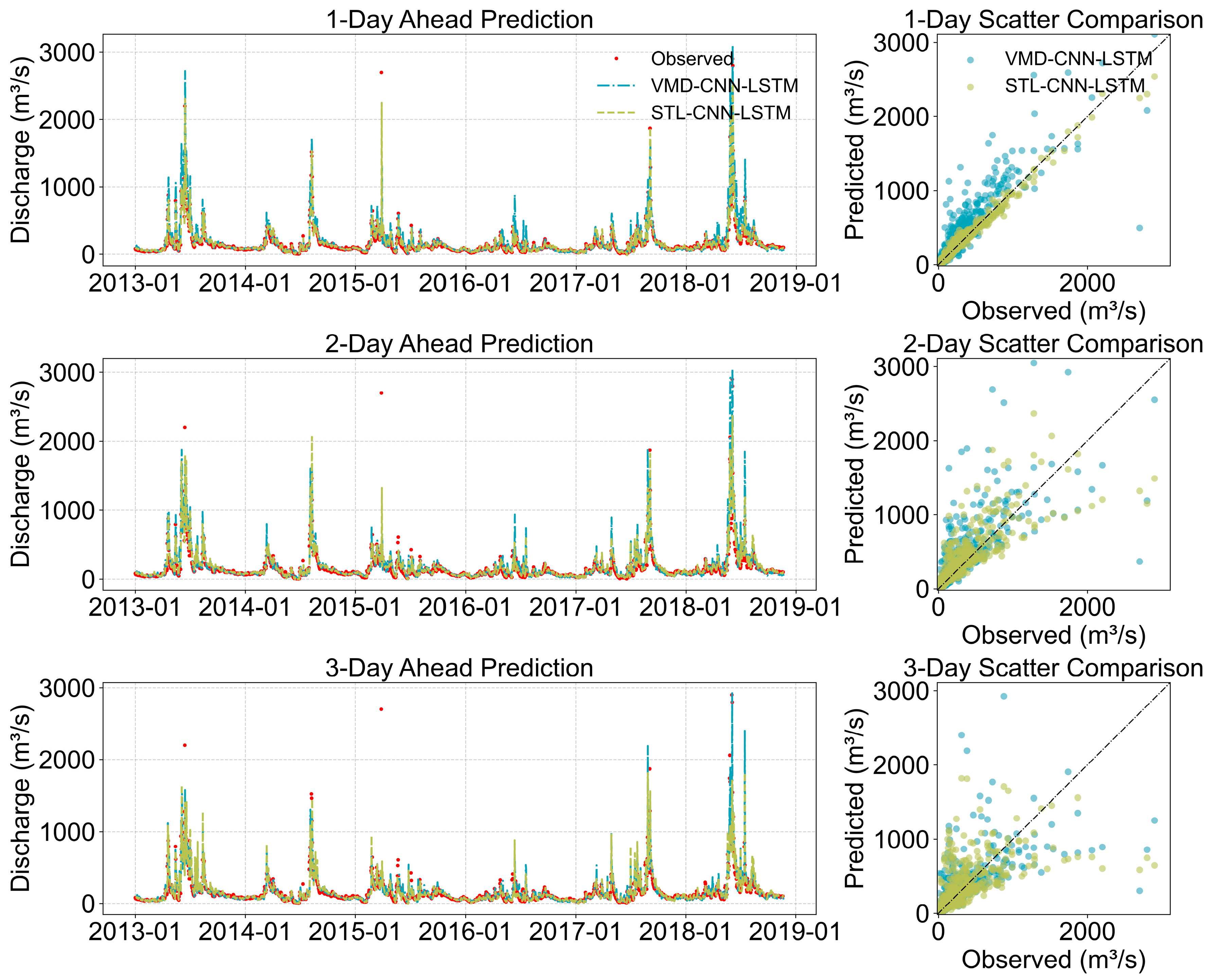
Furthermore, an in-depth comparative analysis was conducted between the STL-CNN-LSTM and VMD-CNN-LSTM models. The results indicate that the STL-CNN-LSTM model demonstrates marginally superior performance over the VMD-CNN-LSTM model. This advantage is consistently reflected across three key evaluation metrics: MAE, RMSE, and NSE. The enhanced performance in these measures suggests that the STL decomposition method conveys a distinct advantage in runoff prediction tasks. Figure 6 illustrates the hybrid prediction framework integrating both decomposition techniques, presenting time-series comparisons between predicted and observed runoff as well as scatter density plots for assessing predictive accuracy. Visual inspection confirms that the decomposition-based models achieve visibly improved agreement with observed values compared to the baseline CNN-LSTM model. Notably, predictions using STL decomposition exhibit tighter clustering along the 1:1 line relative to those using VMD, indicating its stronger capability in capturing runoff dynamics.
In summary, adding decomposition methods to the CNN-LSTM model could enhance runoff prediction accuracy. STL, a time series decomposition method, outperformed VMD, a time-frequency signal decomposition method, in boosting prediction performance. STL better extracted seasonal and trend components from runoff data, becoming a better choice for optimizing CNN-LSTM models.

3.3. Comparative Predictive Performance Across Models

Figure 7 presents a comparative analysis of model performance across different lead times (1, 2, and 3 days) using the MAE and Relative Error (RE) as metrics. The models evaluated include LSTM, CNN-LSTM, VMD-CNN-LSTM, and STL-CNN-LSTM. Each plot displays the predictive performance of runoff forecasting models, with different size symbols representing various sample sizes (e.g., 1, 875, and 1750 samples) and different shapes indicating different model types. Figure 7 demonstrates that the STL-CNN-LSTM model delivers optimal performance for one and two-day forecast periods. This is corroborated by consistently low RE and MAE values during prediction, underscoring the model’s effectiveness in accurately forecasting outcomes over shorter lead times. At three-day lead times, the STL-CNN-LSTM model maintains robust accuracy across most runoff ranges but shows declining precision above 2000 m3/s (data are rendered in red within Figure 7). This is likely due to the increased uncertainty inherent in longer forecast periods, which can hinder the model’s capability to accurately capture extreme event dynamics.
It is noteworthy that the majority of the runoff values are concentrated within the range of 1–500 m3/s (data are rendered in blue within Figure 7), where the STL-CNN-LSTM model demonstrates exceptional prediction capabilities. Although the STL-CNN-LSTM model exhibits moderate peak runoff accuracy at 3-day lead times, its overall performance remains superior due to exceptional consistency across most flow regimes. This substantiates the model’s robustness and reliability under hydrologically diverse conditions.
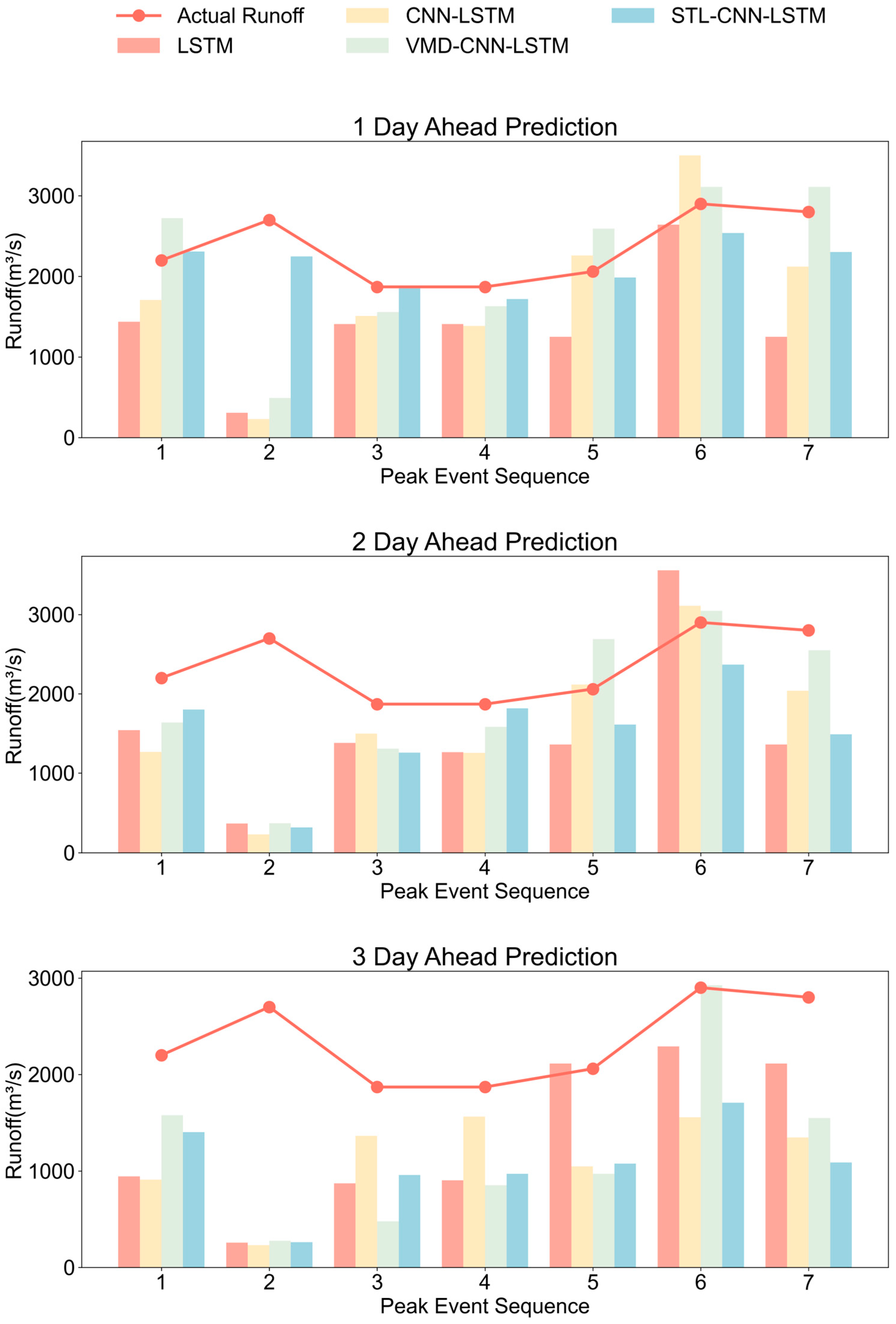
To evaluate the predictive performance of the four models regarding runoff peaks across different lead times, the seven largest peak runoff events within the test set were selected for detailed analysis.
As illustrated in Figure 8, a comparison of flood peak predictions across multiple models during representative events reveals that the STL-CNN-LSTM model generally demonstrates superior accuracy in capturing peak values. Nevertheless, despite its overall enhanced performance in runoff peak forecasting, the STL-CNN-LSTM model exhibits certain deficiencies in predicting specific individual peaks. For instance, in the 3-day ahead prediction, it produced a peak runoff value of 1401 m3/s, significantly underestimating the observed peak of 2200 m3/s. In contrast, the standalone LSTM model shows relatively greater prediction stability compared to the hybrid frameworks under certain conditions. However, for complex runoff processes, the predictive performance of the LSTM model approximates that of a naive model, displaying noticeable time lags between predictions and observations. Specifically, its higher peak predictions tend to align closely with preceding high-value measurements, leading to improved agreement with the actual runoff peaks.

4. Discussion

4.1. Forecasting Performance Advantage Analysis of the Proposed Framework

The results demonstrate the efficacy of the proposed STL-CNN-LSTM model within decomposition-based hybrid forecasting frameworks. This approach achieves robust prediction performance, attributable to the following factors: first, because the use of segmented decomposition-based sampling method leads to a decrease in the prediction accuracy; hybrid neural networks integrate the advantages of different neural networks and have been shown to be effective in improving prediction accuracy in recent years [53,55]. The CNN-LSTM coupling significantly enhanced prediction accuracy over standalone LSTM, evidenced by progressive NSE improvements of 4.79%, 3.69%, and 2.12% for 1 to 3 day runoff forecasts, respectively. The CNN-LSTM’s runoff prediction superiority stems from its synergistic resolution of the “spatial heterogeneity-temporal persistence paradox” [56]: convolutional layers hierarchically abstract localized spatial features, while LSTM gates capture irregular temporal dynamics [57]. According to the seminal model evaluation guidelines by Moriasi et al. (2007) [58], NSE values above 0.75 are considered ‘very good’, while values between 0.65 and 0.75 are deemed ‘satisfactory’. Therefore, our CNN-LSTM model delivers ‘very good’ performance for the first two days and a ‘satisfactory’ performance on Day 3, effectively extending the reliable prediction horizon compared to the LSTM model, which only achieves ‘very good’ performance on Day 1.
Second, STL decomposition explicitly isolates seasonal and trend components via iterative smoothing and cyclic subseries extraction. This aligns with runoff sequences’ intrinsic hydrological periodicity, and seasonal component removal yields stabilized series with enhanced model ability for predictive frameworks [59]. In contrast, VMD’s signal-adaptive decomposition into IMFs may inadvertently disperse critical hydrological features across multiple bandwidth-limited components. Moreover, its frequency-domain methodology risks introducing phase distortions or over-decomposition artifacts that compromise prediction accuracy in hydrological applications [60,61].
In addition, the multi-input neural network critically contributes to the predictive advantage of the proposed framework. By establishing direct functional mappings between runoff subsequences and original series samples, this architecture significantly enhances model accuracy. Our framework utilizes original runoff data as the response variable, while the segmented decomposition methodology rigorously precludes future information incorporation during sampling. It is more rigorous and consistent with the practical application scenarios. By establishing direct the mappings relationship between the runoff subsequence samples and the original sequence samples, this framework effectively avoided the problem of prediction error accumulation in the traditional decomposition-prediction framework, thereby improving the prediction accuracy of the model [7,14]. For lead times of 1 to 3 days, our STL-CNN-LSTM model significantly exceeds the NSE threshold of 0.75. Furthermore, its accuracy is competitive with that reported in recent studies on deep learning for runoff prediction [62,63,64].

4.2. Uncertainties and Limitations

Although the proposed STL-CNN-LSTM model demonstrates strong capabilities in precipitation-runoff modeling, several limitations still persist. First, that while STL-CNN-LSTM outperforms LSTM overall, its continued applicability across all conditions requires additional investigation. Second, emerging explainable frameworks including SHAP (SHapley Additive exPlanations [65]) values and gradient-based saliency analysis can partially decode input-prediction causality in neural networks, enhancing hydrological model interpretability [66]—due to the limitation of space, however, this article does not conduct a more in-depth study. Finally, adopting the MSE as the loss function prioritized overall runoff series prediction at the expense of peak/valley accuracy. Runoff variations induced by extreme precipitation events, anthropogenic water usage, or reservoir regulation operations may introduce uncertainties in framework performance. This study employed STL and VMD for input signal preconditioning, targeting abrupt change mitigation in hydrological series. Currently, studies are exploring hybrid models combining both the STL and VMD methods, such as using STL to extract trend and seasonal terms, while using VMD to process the residuals, in order to combine the advantages of the two to improve the prediction accuracy of the long foresight period [59]. Future work will investigate STL-VMD applications in hydrological time series to elucidate underlying hydrological cycle mechanisms revealed by the model.

5. Conclusions

This study addresses the dual objectives of enhancing practicability and prediction performance in decomposition-based hybrid runoff forecasting by proposing an innovative segmented decomposition framework. Within this framework, we implement an STL-CNN-LSTM model where runoff series undergo stepwise STL decomposition to extract prediction samples derived from trend, seasonality, and remainder subsequences. These decomposed features are subsequently fed into a multi-input CNN-LSTM neural network to produce final runoff predictions. Validation through medium-term runoff forecasting in the Weihe River basin confirms notable performance improvements. The CNN-LSTM hybrid achieves substantial improvements over standalone LSTM, with NSE enhancements of 5.13% (day 1), 3.95% (day 2), and 2.94% (day 3) across lead times. The STL-CNN-LSTM model demonstrated superior performance, achieving optimal NSE values of 0.96 (day 1), 0.83 (day 2), and 0.80 (day 3)—representing significant improvements of 23.08%, 9.21%, and 17.65%, respectively, over the standalone LSTM model.
The proposed framework effectively simulates runoff during both high-flow and low-flow periods, demonstrating robust applicability throughout annual hydrologic cycles regardless of seasonal variations. Moreover, the utility of the STL-CNN-LSTM model extends beyond the specific case study and simulation targets presented here. Given adequate observational data, the framework also supports hydrological simulations of groundwater storage dynamics and water quality parameters.

Author Contributions

Conceptualization, L.L. and R.M.; methodology, R.M.; software, R.M., Y.C. and Q.A.; writing and editing, R.M., L.L. and X.L. All authors contributed to the editing of the manuscript. All authors have read and agreed to the published version of the manuscript.

Funding

This research was jointly funded by the National Natural Science Foundation of China (Grant number: 52379054) and the 2115 Talent Development Program of China Agricultural University (Grant Number: 00109019).

Data Availability Statement

Meteorological data, including precipitation, air temperature, surface pressure, specific humidity, downward longwave radiation, and downward shortwave radiation, were sourced from the CMFD (https://www.tpdc.ac.cn/home). The NDVI dataset were obtained from the MOD13C2 product (https://ladsweb.modaps.eosdis.nasa.gov/missions-and-measurements/products/MOD13C2, accessed on 11 September 2025). Daily runoff records (1990–2019) for key mainstream stations in the Weihe River Basin were obtained from the Annual hydrological report, P. R. China.

Acknowledgments

The authors are grateful to Moderate Resolution Imaging Spectroradiometer (MODIS) team, The China Meteorological Forcing Data (CMFD) group, for making the data freely available.

Conflicts of Interest

The authors declare no conflicts of interest.

References

  1. Feng, Z.; Niu, W.; Tang, Z.; Jiang, Z.; Xu, Y.; Liu, Y.; Zhang, H. Monthly runoff time series prediction by variational mode decomposition and support vector machine based on quantum-behaved particle swarm optimization. J. Hydrol. 2020, 583, 124627. [Google Scholar] [CrossRef]
  2. He, X.X.; Luo, J.G.; Zuo, G.G.; Xie, J.C. Daily Runoff Forecasting Using a Hybrid Model Based on Variational Mode Decomposition and Deep Neural Networks. Water Resour. Manag. 2019, 33, 1571–1590. [Google Scholar] [CrossRef]
  3. Shiri, J.; Kisi, O. Short-term and long-term streamflow forecasting using a wavelet and neuro-fuzzy conjunction model. J. Hydrol. 2010, 394, 486–493. [Google Scholar] [CrossRef]
  4. Liu, Y.; Gupta, H.V. Uncertainty in hydrologic modeling: Toward an integrated data assimilation framework. Water Resour. Res. 2007, 43, W07401. [Google Scholar] [CrossRef]
  5. Kratzert, F.; Klotz, D.; Brenner, C.; Schulz, K.; Herrnegger, M. Rainfall–runoff modelling using Long Short-Term Memory (LSTM) networks. Hydrol. Earth Syst. Sci. 2018, 22, 6005–6022. [Google Scholar] [CrossRef]
  6. Xu, Y.; Hu, C.; Wu, Q.; Jian, S.; Li, Z.; Chen, Y.; Zhang, G.; Zhang, Z.; Wang, S. Research on particle swarm optimization in LSTM neural networks for rainfall-runoff simulation. J. Hydrol. 2022, 608, 127553. [Google Scholar] [CrossRef]
  7. Nazeer, A.; Maskey, S.; Skaugen, T.; McClain, M.E. Simulating the hydrological regime of the snow fed and glaciarised Gilgit Basin in the Upper Indus using global precipitation products and a data parsimonious precipitation-runoff model. Sci. Total Environ. 2022, 802, 149872. [Google Scholar] [CrossRef]
  8. Zhao, S.; Fang, J.; Wang, Y.; Zhang, Y.; Zhou, Y.; Zhuo, S. Construction of three-dimensional mesoporous carbon nitride with high surface area for efficient visible-light-driven hydrogen evolution. J. Colloid Interface Sci. 2020, 561, 601–608. [Google Scholar] [CrossRef] [PubMed]
  9. Chen, I.; Chang, L.; Chang, F. Exploring the spatio-temporal interrelation between groundwater and surface water by using the self-organizing maps. J. Hydrol. 2018, 556, 131–142. [Google Scholar] [CrossRef]
  10. He, X.; Luo, J.; Li, P.; Zuo, G.; Xie, J. A Hybrid Model Based on Variational Mode Decomposition and Gradient Boosting Regression Tree for Monthly Runoff Forecasting. Water Resour. Manag. 2020, 34, 865–884. [Google Scholar] [CrossRef]
  11. Xiang, Z.; Yan, J.; Demir, I. A Rainfall-Runoff Model with LSTM-Based Sequence-to-Sequence Learning. Water Resour. Res. 2020, 56, e2019WR025326. [Google Scholar] [CrossRef]
  12. Malakoutian, M.M.A.; Samaei, S.Y.; Khaksar, M.; Malakoutian, Y. A prediction of future flows of ephemeral rivers by using stochastic modeling (AR autoregressive modeling). Sustain. Oper. Comput. 2022, 3, 330–335. [Google Scholar] [CrossRef]
  13. Wang, Z.; Xu, N.; Bao, X.; Wu, J.; Cui, X. Spatio-temporal deep learning model for accurate streamflow prediction with multi-source data fusion. Environ. Modell. Softw. 2024, 178, 106091. [Google Scholar] [CrossRef]
  14. Zuo, G.; Luo, J.; Wang, N.; Lian, Y.; He, X. Decomposition ensemble model based on variational mode decomposition and long short-term memory for streamflow forecasting. J. Hydrol. 2020, 585, 124776. [Google Scholar] [CrossRef]
  15. Qiao, X.; Peng, T.; Sun, N.; Zhang, C.; Liu, Q.; Zhang, Y.; Wang, Y.; Shahzad Nazir, M. Metaheuristic evolutionary deep learning model based on temporal convolutional network, improved aquila optimizer and random forest for rainfall-runoff simulation and multi-step runoff prediction. Expert Syst. Appl. 2023, 229, 120616. [Google Scholar] [CrossRef]
  16. Valipour, M.; Banihabib, M.E.; Behbahani, S.M.R. Comparison of the ARMA, ARIMA, and the autoregressive artificial neural network models in forecasting the monthly inflow of Dez dam reservoir. J. Hydrol. 2013, 476, 433–441. [Google Scholar] [CrossRef]
  17. Huang, S.; Chang, J.; Huang, Q.; Chen, Y. Monthly streamflow prediction using modified EMD-based support vector machine. J. Hydrol. 2014, 511, 764–775. [Google Scholar] [CrossRef]
  18. Man, Y.; Yang, Q.; Shao, J.; Wang, G.; Bai, L.; Xue, Y. Enhanced LSTM Model for Daily Runoff Prediction in the Upper Huai River Basin, China. Engineering. 2023, 24, 229–238. [Google Scholar] [CrossRef]
  19. Meng, E.; Huang, S.; Huang, Q.; Fang, W.; Wu, L.; Wang, L. A robust method for non-stationary streamflow prediction based on improved EMD-SVM model. J. Hydrol. 2019, 568, 462–478. [Google Scholar] [CrossRef]
  20. Yao, Z.; Wang, Z.; Wang, D.; Wu, J.; Chen, L. An ensemble CNN-LSTM and GRU adaptive weighting model based improved sparrow search algorithm for predicting runoff using historical meteorological and runoff data as input. J. Hydrol. 2023, 625, 129977. [Google Scholar] [CrossRef]
  21. Uttarwar, S.B.; Lerch, S.; Avesani, D.; Majone, B. Performance assessment of neural network models for seasonal weather forecast postprocessing in the Alpine region. Adv. Water Resour. 2025, 204, 105061. [Google Scholar] [CrossRef]
  22. Kachroo, R.K.; Natale, L. Non-linear modelling of the rainfall-runoff transformation. J. Hydrol. 1992, 135, 341–369. [Google Scholar] [CrossRef]
  23. Guo, J.; Liu, Y.; Zou, Q.; Ye, L.; Zhu, S.; Zhang, H. Study on optimization and combination strategy of multiple daily runoff prediction models coupled with physical mechanism and LSTM. J. Hydrol. 2023, 624, 129969. [Google Scholar] [CrossRef]
  24. Parisouj, P.; Jun, C.; Bateni, S.M.; Heggy, E.; Band, S.S. Daily runoff forecasting using novel optimized machine learning methods. Results Eng. 2024, 24, 103319. [Google Scholar] [CrossRef]
  25. Wu, S.; Dong, Z.; Guzmán, S.M.; Conde, G.; Wang, W.; Zhu, S.; Shao, Y.; Meng, J. Two-step hybrid model for monthly runoff prediction utilizing integrated machine learning algorithms and dual signal decompositions. Ecol. Inform. 2024, 84, 102914. [Google Scholar] [CrossRef]
  26. Xu, P.; Wang, D.; Wang, Y.; Singh, V.P. A Stepwise and Dynamic C-Vine Copula–Based Approach for Nonstationary Monthly Streamflow Forecasts. J. Hydrol. Eng. 2022, 27, 4021043. [Google Scholar] [CrossRef]
  27. Zhang, X.; Peng, Y.; Zhang, C.; Wang, B. Are hybrid models integrated with data preprocessing techniques suitable for monthly streamflow forecasting? Some experiment evidences. J. Hydrol. 2015, 530, 137–152. [Google Scholar] [CrossRef]
  28. Liu, J.; Xu, T.; Lu, C.; Yang, J.; Xie, Y. Variational mode decomposition coupled LSTM with encoder-decoder framework: An efficient method for daily streamflow forecasting. Earth Sci. Inform. 2024, 18, 38. [Google Scholar] [CrossRef]
  29. Bai, Y.; Chen, Z.; Xie, J.; Li, C. Daily reservoir inflow forecasting using multiscale deep feature learning with hybrid models. J. Hydrol. 2016, 532, 193–206. [Google Scholar] [CrossRef]
  30. Luo, Y.; Dong, Z.; Liu, Y.; Wang, X.; Shi, Q.; Han, Y. Research on stage-divided water level prediction technology of rivers-connected lake based on machine learning: A case study of Hongze Lake, China. Stoch. Environ. Res. Risk Assess. 2021, 35, 2049–2065. [Google Scholar] [CrossRef]
  31. Luo, X.; Yuan, X.; Zhu, S.; Xu, Z.; Meng, L.; Peng, J. A hybrid support vector regression framework for streamflow forecast. J. Hydrol. 2019, 568, 184–193. [Google Scholar] [CrossRef]
  32. Lei, Q.; Gao, P.; Li, J. A Monthly Runoff Forecast Model Combining Time Series Decomposition and CNN-LSTM. J. Yangtze River Sci. Res. Inst. 2023, 40, 49–54. [Google Scholar]
  33. Xu, Z.; Mo, L.; Zhou, J.; Fang, W.; Qin, H. Stepwise decomposition-integration-prediction framework for runoff forecasting considering boundary correction. Sci. Total Environ. 2022, 851, 158342. [Google Scholar] [CrossRef]
  34. Okkan, U.; Samui, P. Modeling of Watershed Runoff Using Discrete Wavelet Transform and Support Vector Machines. Fresenius Environ. Bull. 2012, 21, 3971–3986. [Google Scholar]
  35. Parisouj, P.; Jun, C.; Bateni, S.M.; Heggy, E.; Band, S.S. Machine learning models coupled with empirical mode decomposition for simulating monthly and yearly streamflows: A case study of three watersheds in Ontario, Canada. Eng. Appl. Comput. Fluid. Mech. 2023, 17, 2242445. [Google Scholar] [CrossRef]
  36. Zhang, G.P.; Qi, M. Neural network forecasting for seasonal and trend time series. Eur. J. Oper. Res. 2005, 160, 501–514. [Google Scholar] [CrossRef]
  37. Du, K.; Zhao, Y.; Lei, J. The incorrect usage of singular spectral analysis and discrete wavelet transform in hybrid models to predict hydrological time series. J. Hydrol. 2017, 552, 44–51. [Google Scholar] [CrossRef]
  38. Fang, W.S.K.Q. Examining the applicability of different sampling techniques in the development of decomposition-based streamflow forecasting models. J. Hydrol. 2019, 568, 534–550. [Google Scholar] [CrossRef]
  39. Quilty, J.; Adamowski, J. Addressing the incorrect usage of wavelet-based hydrological and water resources forecasting models for real-world applications with best practices and a new forecasting framework. J. Hydrol. 2018, 563, 336–353. [Google Scholar] [CrossRef]
  40. Tan, Q.; Lei, X.; Wang, X.; Wang, H.; Wen, X.; Ji, Y.; Kang, A. An adaptive middle and long-term runoff forecast model using EEMD-ANN hybrid approach. J. Hydrol. 2018, 567, 767–780. [Google Scholar] [CrossRef]
  41. Wang, Y.; Wu, L. On practical challenges of decomposition-based hybrid forecasting algorithms for wind speed and solar irradiation. Energy. 2016, 112, 208–220. [Google Scholar] [CrossRef]
  42. Chen, Z.; Zhang, H.; Lu, H.; Lyu, F.; Lyu, H.; Gao, R.; Chen, Y.; Wu, M. Evolution of the proto-Weihe River system during the Eocene–Oligocene: Evidence from sediment provenance of the Weihe Basin. Geomorphology. 2025, 473, 109616. [Google Scholar] [CrossRef]
  43. Zhang, Y.; Zhang, B.; Ma, B.; Yao, R.; Wang, L. Evaluation of the water conservation capacity of the Weihe River Basin based on the Integrated Valuation of Ecosystem Services and Tradeoffs model. Ecohydrology 2022, 15, e2465. [Google Scholar] [CrossRef]
  44. Liu, L.; Rui, H. Exploration on Structural Characteristics of the Weihe Basin and Its Evolution. J. Geomech. 2018, 24, 60–69. [Google Scholar]
  45. Fan, J.; Yu, G.; Zhao, M.; Zong, H. Addressing multi-scale temporal variability: Deep integration and application of the CNN and transformer model in monthly streamflow prediction. Expert Syst. Appl. 2025, 292, 128658. [Google Scholar] [CrossRef]
  46. Tang, G.; Wood, A.W.; Swenson, S. On Using AI-Based Large-Sample Emulators for Land/Hydrology Model Calibration and Regionalization. Water Resour. Res. 2025, 61, e2024WR039525. [Google Scholar] [CrossRef]
  47. He, J.; Yang, K.; Tang, W.; Lu, H.; Qin, J.; Chen, Y.; Li, X. China Meteorological Forcing Dataset (1979–2018); National TPDC ed:National Tibetan Plateau Data Center: Beijing, China, 2015. [Google Scholar]
  48. Dragomiretskiy, K.; Zosso, D. Variational Mode Decomposition. IEEE Trans. Signal Process. 2014, 62, 531–544. [Google Scholar] [CrossRef]
  49. Cleveland, R.B.; Cleveland, W.S. STL: A seasonal-trend decomposition procedure based on Loess. J. Off. Stat. 1990, 6, 3–73. [Google Scholar]
  50. Wen, S.; Wang, H.; Qian, J.; Men, X. A novel combined model based on echo state network optimized by whale optimization algorithm for blast furnace gas prediction. Energy. 2023, 279, 128048. [Google Scholar] [CrossRef]
  51. Guo, Y.; Xu, Y.; Sun, M.; Xie, J. Multi-step-ahead forecast of reservoir water availability with improved quantum-based GWO coupled with the AI-based LSSVM model. J. Hydrol. 2021, 597, 125769. [Google Scholar] [CrossRef]
  52. Guo, Z.; Zhao, W.; Lu, H.; Wang, J. Multi-step forecasting for wind speed using a modified EMD-based artificial neural network model. Renew. Energy. 2012, 37, 241–249. [Google Scholar] [CrossRef]
  53. Deng, H.Q.; Chen, W.J.; Huang, G.R. Deep insight into daily runoff forecasting based on a CNN-LSTM model. Nat. Hazards 2022, 113, 1675–1696. [Google Scholar] [CrossRef]
  54. Wang, Y.; Li, J.; Wang, S.; Zhang, H.; Yang, L.; Wu, W. Extreme Short-Term Prediction of Unmanned Surface Vessel Nonlinear Motion Under Waves. J. Mar. Sci. Eng. 2025, 13, 610. [Google Scholar] [CrossRef]
  55. Zhou, F.; Chen, Y.; Liu, J. Application of a New Hybrid Deep Learning Model That Considers Temporal and Feature Dependencies in Rainfall–Runoff Simulation. Remote Sens. 2023, 15, 1395. [Google Scholar] [CrossRef]
  56. Li, B.; Li, R.; Sun, T.; Gong, A.; Tian, F.; Khan, M.Y.A.; Ni, G. Improving LSTM hydrological modeling with spatiotemporal deep learning and multi-task learning: A case study of three mountainous areas on the Tibetan Plateau. J. Hydrol. 2023, 620, 129401. [Google Scholar] [CrossRef]
  57. Li, T.; Hua, M.; Wu, X.U. A Hybrid CNN-LSTM Model for Forecasting Particulate Matter (PM2.5). IEEE Access 2020, 8, 26933–26940. [Google Scholar] [CrossRef]
  58. Moriasi, D.N.; Arnold, J.G.; Liew, M.W.V.; Bingner, R.L.; Harmel, R.D.; Veith, T.L. Model Evaluation Guidelines for Systematic Quantification of Accuracy in Watershed Simulations. Trans. ASABE. 2007, 50, 885–900. [Google Scholar] [CrossRef]
  59. Yang, H.; Li, W. Data Decomposition, Seasonal Adjustment Method and Machine Learning Combined for Runoff Prediction: A Case Study. Water Resour. Manag. 2023, 37, 557–581. [Google Scholar] [CrossRef]
  60. Chen, Y.; Xue, M.; Zhang, J.; Ou, R.; Zhang, Q.; Kuang, P. DetectDUI: An In-Car Detection System for Drink Driving and BACs. IEEE/ACM Trans. Netw. 2022, 30, 896–910. [Google Scholar] [CrossRef]
  61. Zheng, T.; Chen, Z.; Cai, C.; Luo, J.; Zhang, X. V2iFi: In-Vehicle Vital Sign Monitoring via Compact RF Sensing. Proc. ACM Interact. Mob. Wearable Ubiquitous Technol. 2020, 4, 70. [Google Scholar] [CrossRef]
  62. Wang, W.; Gao, J.; Liu, Z.; Li, C. A hybrid rainfall-runoff model: Integrating initial loss and LSTM for improved forecasting. Front. Environ. Sci. 2023, 11, 1261239. [Google Scholar] [CrossRef]
  63. Yu, C.; Hu, D.; Shao, H.; Dai, X.; Liu, G.; Wu, S. Runoff simulation driven by multi-source satellite data based on hydrological mechanism algorithm and deep learning network. J. Hydrol. Reg. Stud. 2024, 52, 101720. [Google Scholar] [CrossRef]
  64. Yue, J.; Zhou, L.; Du, J.; Zhou, C.; Nimai, S.; Wu, L.; Ao, T. Runoff Simulation in Data-Scarce Alpine Regions: Comparative Analysis Based on LSTM and Physically Based Models. Water 2024, 16, 2161. [Google Scholar] [CrossRef]
  65. Lundberg, S.M.; Lee, S. A unified approach to interpreting model predictions. In Proceedings of the 31st International Conference on Neural Information Processing Systems, Long Beach, CA, USA, 4–9 December 2017; Curran Associates Inc.: Red Hook, NY, USA, 2017; pp. 4768–4777. [Google Scholar]
  66. Wang, S.; Peng, H. Multiple spatio-temporal scale runoff forecasting and driving mechanism exploration by K-means optimized XGBoost and SHAP. J. Hydrol. 2024, 630, 130650. [Google Scholar] [CrossRef]
Figure 1. Location, topography, and hydrometeorological station distribution of the Weihe River Basin.
Water 17 02718 g001
Figure 2. A progressive decomposition methodology chart.
Water 17 02718 g002
Figure 3. The structure of the CNN-LSTM model.
Water 17 02718 g003
Figure 4. Decomposition ensemble models for runoff forecasting.
Water 17 02718 g004
Figure 5. Comparison of discharge prediction using LSTM and CNN-LSTM.
Water 17 02718 g005
Figure 6. Comparison of discharge prediction using VMD-CNN-LSTM and STL-CNN-LSTM.
Water 17 02718 g006
Figure 7. Comparative model performance across 1–3 day lead times using MAE and RE. Runoff magnitude visualization via blue (low runoff: <500 m3/s) to red (peak runoff: >2500 m3/s) color scaling and different shapes indicating different model types. Symbol area is proportional to the number of observations per runoff bin, facilitating visual assessment of data representativeness.
Water 17 02718 g007
Figure 8. Peak flow forecasting of different models. The x-axis (Peak Event Sequence) represents the chronological order of the seven largest peak flow events identified within the test period.
Water 17 02718 g008
Table 1. Water Gauge Information.
Water Gauge IDWater Gauge NameLongitude (°E)Latitude (°N)Elevation (m a.s.l.)Basin Area Controlled By Individual Water Gauge (km2)
W1Beidao105.9734.62138924,871
W2Weijiabao107.7034.3049637,012
W3Xianyang108.7034.3238746,827
W4Lintong109.2034.4335497,299
W5Huaxian109.7734.58339106,498
Table 2. The prediction accuracy of LSTM model and CNN-LSTM model.
Model CategoryPerformance Assessment1st-Day2nd-Day3rd-Day
LSTMMAE (m3/s)37.4744.4356.18
RMSE (m3/s)101.06104.84120.56
NSE0.780.760.68
CNN-LSTMMAE (m3/s)41.4745.1849.72
RMSE (m3/s)92.1697.98117.75
NSE0.820.790.70
Note: where 1st-day is the first day; 2nd-day is the second day; 3rd-day is the third day.
Table 3. The prediction accuracy of VMD-CNN-LSTM and STL-CNN-LSTM model.
Model CategoryPerformance Assessment1st-Day2nd-Day3rd-Day
VMD-CNN-LSTMMAE (m3/s)29.6546.5849.63
RMSE (m3/s)65.1896.98112.63
NSE0.910.790.71
STL-CNN-LSTMMAE (m3/s)19.0132.4534.01
RMSE (m3/s)42.4193.8287.14
NSE0.960.830.80
Disclaimer/Publisher’s Note: The statements, opinions and data contained in all publications are solely those of the individual author(s) and contributor(s) and not of MDPI and/or the editor(s). MDPI and/or the editor(s) disclaim responsibility for any injury to people or property resulting from any ideas, methods, instructions or products referred to in the content.