Abstract
Subsea pipelines with intermittent spanwise arrangements are commonly encountered in offshore engineering, yet their complex hydrodynamic interactions remain insufficiently understood. In this study, three-dimensional numerical simulations were conducted to investigate the hydrodynamics of intermittently spanning cylinders at a Reynolds number of 40,250. The hydrodynamic coefficients and flow fields of cylinders with different gap ratios e/D, total spanning ratios L/H, and individual spanning ratios l/D were investigated (where e is the gap height, D is the diameter of the cylinder, L is the total spanning length, H is the length of the cylinder, and l is the individual spanning length). Moreover, this work validates the applicability of existing hydrodynamic prediction formulas for spanning cylinders under complex spanning conditions, as proposed by previous researchers. Numerical results show that the existing formulas can accurately predict the drag coefficient of spanning cylinders under different uniform l/D ratios, but it fails to provide reliable predictions for the lift coefficient . These findings provide critical insights for optimizing the design of subsea pipelines and marine structures with intermittent spanwise arrangements.
1. Introduction
Steady incoming flow past a smooth circular cylinder (referred to as flow past a circular hereafter) has been a classical problem in fluid mechanics for more than a century, given its fundamental significance and practical applications. Due to its complex hydrodynamic phenomena, such as flow separation, vortex shedding, and the evolution characteristics of the flow structure, a large number of experimental and numerical simulation studies have been conducted. And a wealth of data and results have recently been obtained [1,2]. It is well known that the benchmarking case is mainly controlled by the Reynolds number Re, defined as Re = UD/ν, where U is the characteristic velocity, D is the diameter of cylinder, and ν is the fluid kinematic viscosity. Despite its geometrically simple structure, many flow regimes are observed as increasing Re. For instance, two-dimensional vortex shedding begins to occur at Re ≈ 47, the wake transitions from two-dimensional to three-dimensional at Re ≈ 190, and the phenomenon of drag crisis caused by the transition of the boundary layer of the cylinder [1]. To date, there have been numerous investigations on the evolution characteristics of flow fields and the hydrodynamic characteristics of the fluid around a cylinder in an unbounded flow field at different Reynolds numbers [1,2,3,4].
Compared to the problem of flow past a circular cylinder in an unbounded flow field, the wake structure of a near-wall cylinder is more complex, and the interaction between the wall boundary layer and the wake behind a cylinder will profoundly alter the hydrodynamic characteristics of the cylinder. For more than half a century, extensive experiments and numerical simulations have been conducted on the forces and flow-field structure of the near-wall cylinder. Bearman and Zdravkovich [5] investigated the wake patterns of a cylinder placed above a flat plate at different heights, as well as the pressure distribution along the surface of the cylinder through wind tunnel experiments, with the inflow boundary layer thickness being 0.8D in the experiments. The results of the experiment indicated that in the case of a small gap ratio e/D (where e is the distance of the cylinder from the wall), the vortex shedding in the wake will be suppressed, while the presence of the wall significantly alters the symmetry of the pressure on the surface of the cylinder. Zdravkovich [6] measured drag force and lift force acting on a near-wall circular cylinder in subcritical flow. The experimental results show that when the cylinder is placed outside of the incoming boundary layer, the average drag coefficient increases with the increase in the gap ratio e/D, and approaches in an unbounded flow field when the gap ratio e/D is greater than 2. When the cylinder is placed within the boundary layer, the average drag coefficient is mainly influenced by the thickness of the boundary layer, while the average lift coefficient is primarily controlled by the gap ratio. Further investigations have found that the mean drag coefficient and the mean lift coefficient both strongly depend on the gap ratio e/D and are affected by the boundary layer thickness. Within the gap ratio range of e/D from 0.2 to 0.3, the shedding of the cylinder’s trailing vortex is suppressed; when the gap ratio of e/D is in the range of 0.5 to 0.6, the suppression of the vortices near the wall weakens, and the mean drag coefficient reaches its maximum value, which is approximately 1.2 times of the mean drag coefficient of the cylinder in an unbounded flow field under the same conditions [6,7,8]. In addition, the wake structure behind the near-wall cylinder is asymmetric. Two peaks are observed in the variation in mean lift coefficient as the gap ratio e/D changes. One peak occurs at e/D = 0, where the suction on the surface of the cylinder is dominant, and the other peak occurs at approximately e/D = 0.1, where the stagnation pressure is dominant [9].
In actual marine engineering, local scour often occurs at multiple positions along the pipelines and cables. Furthermore, the actual seabed can be uneven, causing the submarine cables to form multiple intermittent spanning sections, with adjacent spanning being supported by the seabed. The spanning distribution of the cylinder will dramatically alter the hydrodynamic forces acting on them, and its force characteristics involve obvious three-dimensional features, which significantly affect the assessment of the on-bottom stability of the cables [10,11]. Griffiths et al. [12] conducted a parametric study through two-dimensional and three-dimensional numerical simulations to explore the hydrodynamic characteristics of non-uniformly spanning cylindrical structures under combined wave and current conditions, quantifying the variation in hydrodynamic loads along the axial direction of the cylinder. Sollund et al. [13] investigated the dynamic response of offshore pipelines in free spans, and derived a novel semi-analytical method for calculating the dynamic response of multi-span pipelines. In addition, Teng et al. [14] studied the effects of the single uniform free spans, multiple regularly spaced free spans, and seabed roughness elements by conducting a large number of experiments under waves. The main purpose aims to quantify the effects of gap height to pipeline diameter ratio and the span length to pipeline diameter ratio on the peak force coefficients. Tong et al. [15,16] used large eddy simulation to study the hydrodynamics of multiple spanning sections near the wall under unidirectional flow. The results show that even a small gap beneath the cylinder can significantly alter the fluid forces acting on the cylinder. Additionally, empirical prediction formulas for the hydrodynamics of spanning cylinders are proposed, as shown in Equations (1) and (2):
Among them, and are the drag coefficient and lift coefficient predicted by empirical formulas, respectively. The superscript S represents the hydrodynamic coefficient of the spanning cylinder, and the superscript NS represents the hydrodynamic coefficient of the non-spanning cylinder. L is the total length of the spanning cylinder, B is the total length of the non-spanning cylinder, and H = L + B is the total length of the cylinder. It is noteworthy that the variables and denote the time-averaged drag and lift coefficients for fully free-spanning cylinder, respectively, while and represent the time-averaged drag and lift coefficients for the fully blocked cylinder.
Although significant achievements have been made in the study of cylindrical flow around spanning structures considering the effects of spanning sections, it is undeniable that there are still certain limitations. Although the above study considered the effects of the total spanning ratio L/H and the gap ratio e/D on the hydrodynamic characteristics of the cylinder, it did not take into account the effect of the individual spanning length l/D on the hydrodynamic characteristics of the cylinder. In addition, the applicability of the existing formula under complex spanning conditions in a cylindrical structure also needs to be examined. Therefore, this work mainly focused on the effect of the single spanning length l/D on the hydrodynamic characteristics of cylinders, while also exploring the applicability of the empirical prediction formula proposed by Tong et al. [16] with different spanning lengths l/D.
With this intention, we have structured the current paper as follows: a short overview and details of the chosen numerical method are presented in Section 2. The main results and discussion are given in Section 3, which includes the hydrodynamic coefficients and flow structure. Finally, Section 4 gives the conclusion of the paper.
2. Numerical Model
Previous similar studies have shown that the large eddy simulation method (LES) has the capability to model high-Reynolds-number flow and resolve the 3D bluff body flow at a relatively lower computational cost Therefore, numerical simulations are performed using the LES model provided by STAR-CCM+ (17.04.008) for investigating the forces acting on the circular cylinder with intermittent spanwise arrangements. It uses a SIMPLEC algorithm for pressure–velocity coupling, which requires Rhie and Chow interpolation to avoid odd–even oscillations [17]. Moreover, the dynamic Smagorinsky model is employed in this research, which automatically updates the Smagorinsky constant over both time and the computational domain and outperforms the conventional Smagorinsky model [18,19].
2.1. Governing Equations
Within the framework of large eddy simulation, the continuity equation and momentum equation for three-dimensional incompressible flow are given as follows:
In the equation, “-” indicates the variable after filtering by a grid filter with a filtering width of Δ, where Δ = V1/3, and V represents the volume of the grid cell. (x1, x2, x3) = (x, y, z) are the Cartesian coordinate components, ui is the velocity component corresponding to the xi direction, t is time, ρ is the fluid density, p is the pressure, and μ is the dynamic viscosity coefficient. τij is the subgrid stress, which characterizes the effect of unresolved small-scale turbulent motions on large-scale flow during the grid filtering process, and can be defined as
Due to the unknown value of subgrid stress term τij, the group of equations is not closed. To close the group of equations, Smagorinsky introduced the Boussinesq hypothesis into large eddy simulation and proposed the relationship between subgrid stress and subgrid eddy viscosity as follows:
where δij is the Kronecker delta, μt is the subgrid-scale turbulent viscosity coefficient, and Sij is the strain rate tensor, which is defined as
To solve the subgrid vortex viscosity coefficient μt, it is necessary to establish a turbulence model. The dynamic Smagorinsky model is employed, and the equation of the dynamic Smagorinsky turbulence model is
where , CS is the coefficient of the Smagorinsky model. In the dynamic Smagorinsky turbulence model, CS is required to be calculated through quadratic filtering, as follows:
where < > indicates spatial averaging of physical quantities, and the calculation formulas of Lij and Mij are as follows:
In the above formula, “~” represents the variable of the secondary filtering with a test filter of width 2Δ. For a detailed introduction of large eddy simulations, please refer to references [20,21].
2.2. Definition of Characteristic Coefficients
For convenience of subsequent descriptions, the characteristic parameters involved in this work are listed here. The drag coefficient CD and lift coefficient CL of the cylinder are defined as follows:
The mean drag coefficient and mean lift coefficient are calculated using the following equations:
In addition, the standard deviation of the drag and lift coefficients is defined as follows:
The pressure coefficient Cp are determined from the time-averaged flow field, where Cp is calculated as
The dimensionless vortex shedding frequency, Strouhal number St, defined as
where FD and FL are the drag force and lift force acting on the unit-length cylinder in the streamwise and cross-flow directions, respectively; U0 represents the free stream velocity outside the boundary layer; A is the cross-sectional area of the cylinder; D is the diameter of the cylinder; p is the pressure distribution on the surface of cylinder; is the reference pressure at the inlet boundary, and f is the vortex-shedding frequency of the cylinder, which is typically obtained by performing fast Fourier transform (FFT) on the time history of the lift coefficient. It is note worthing that similar studies have indicated that the number of the statistical sample N has a critical impact on the accuracy and reliability of the statistical measures of the drag and lift coefficients. Therefore, the statistical period of more than 200 nondimensional time units (defined as ) is adopted in this study (the section enclosed by the green dashed box in Figure 4).
2.3. Geometric Parameters
The hydrodynamic characteristics of cylinder with intermittent spanwise arrangements are mainly influenced by their substructure, which divides the cylinder into spanning and non-spanning sections through multiple blockage blocks, as shown in Figure 1. This work refers to the physical experiment conducted by Teng et al. [22] where the diameter of the cylinder is D, the total length is H, and the total length of the spanning section is L. The distance from the bottom boundary of calculation domain to the cylinder is e. The blocking structure at the lower part of the cylinder is simplified to a rectangular structure, with the blocking block parallel to the length of the cylinder being b and the width being 0.91D. In order to completely block the non-spanning section of the cylinder while accurately capturing the flow structure around the cylinder, a zero-thickness plate is set between the surface of the blocking rectangular structure and the bottom of the cylinder, with a height of e0, where e0 is taken as 0.01D. Therefore, the structural parameters that mainly affect the hydrodynamic coefficients of the cylinder with intermittent spanwise arrangements are the height of the spanning cylinder e/D, the total spanning length L/H, and the individual spanning length of a single spanning section l/D.

Figure 1.
Schematic diagram of a cylinder with intermittent spanwise arrangements.
2.4. Calculation Domain and Boundary Conditions
As is well known, for flow past circular flow problems with Reynolds numbers less than 190, two-dimensional numerical models can provide accurate simulations. However, when the Reynolds number exceeds 190, significant discrepancies arise between the results obtained from two-dimensional and three-dimensional numerical models. Therefore, based on the relevant studies by previous scholars and the research objectives of this paper, the computational domain of this study was established [23,24]. The computational domain, with dimensions of 30D × 10D × 8.7D, is schematically represented in Figure 2. The origin of the Cartesian coordinates is positioned at the center of the circular cross-section of the cylinder, located at the z = 0 plane. The inlet boundary is positioned 10D upstream from the cylinder’s central axis, while the outlet boundary is located 20D downstream from the cylinder’s center. the lower boundary is e away from the bottom of the cylinder, and the upper boundary is 10D away from the lower boundary. The length of the cylinder is 8.7D.
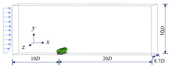
Figure 2.
Schematic diagram of the calculation domain for multiple short-spanning cylindrical sections.
The solution conditions are as follows. Boundary conditions at the entrance:
Boundary conditions for export:
Upper boundary condition:
Lower boundary condition:
Surface conditions of cylindrical and blocking structures:
It is worth noting that to accurately model the boundary layer thickness at the inlet, the velocity profile is defined as follows:
where u* is the friction velocity, defined as u* = κU0/ln(δ/zw), κ is the Karman constant, taken to be 0.41, U0 is the flow velocity outside the boundary layer, δ is the thickness of the boundary layer, and the seabed roughness length zw = d50/12, where d50 represents the median particle size of the seabed sediment, taken as zw = 10−6 m in this study.
2.5. Convergence and Accuracy of the Numerical Model
Firstly, the grid convergence check of the numerical model is given and the grid division schematic is shown in Figure 3. Due to the complex fluid flow near the lower wall of the computational domain, the cylinder, and the blocking structure, local refinement of the grid is carried out in these locations. The expansion rate from the first layer grid thickness near the cylinder surface to the surrounding grid transition does not exceed 1.1.

Figure 3.
Schematic diagram of the mesh.
The main parameters for grid refinement are as follows: (1) the number of grid nodes around the cylinder NC, which is the number of grid nodes around the cylinder; (2) the thickness of the first layer of grid on the cylinder surface Δ1; (3) the number of grid nodes along the length of the cylinder NZ, which is the number of nodes along the longitudinal direction of the cylinder. The grid convergence check is conducted under the conditions of Reynolds number Re = 40,250, boundary layer thickness δ/D = 3, gap height e/D = 0.27, the total spanning ratio L/H = 0.44, and single spanning length l/D = 0.77. The node parameters for the grid convergence check are shown in Table 1, Table 2 and Table 3. The time history of the hydrodynamic coefficients CD and CL are shown in Figure 4, and the dimensionless sampling time of the hydrodynamic coefficients tU0/D is between 100 and 330.

Table 1.
Convergence check of spanwise mesh.

Table 2.
Convergence check of circumferential mesh.

Table 3.
Convergence check of first-layer mesh.
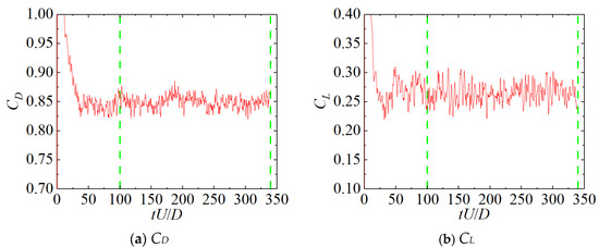
Figure 4.
Time history of the hydrodynamic coefficients.
As shown in Table 1, the number of radial grid nodes NZ was selected as 180, 270, and 360 for the check. By comparing the hydrodynamic coefficients , and CL-rms, it can be observed that the variation in hydrodynamic coefficients is relatively low when the radial grid nodes number NZ is 270 and 360. Therefore, NZ being 270 already meets the convergence requirements.
The circumferential grid parameters for the cylinder are shown in Table 2, with the number of circumferential grid nodes chosen as 120, 160, and 200. By comparing the hydrodynamic coefficients , and CL-rms calculated from the three kinds of grids, it can be observed that the variation in hydrodynamic coefficients is relatively low when the number of circumferential grid nodes changes from 160 to 200. Therefore, the number of circumferential grid nodes NC is taken as 160.
Table 3 presents the convergence check of the first-layer mesh on the surface of cylinder. The dimensionless height Δ1 of the first-layer mesh is set at two values, 0.0002D and 0.0004D. It can be observed that reducing Δ1 from 0.0004D to 0.0002D has little effect on the numerical simulation results, which proves that Δ1 of 0.0004D already meets the convergence requirements.
In order to ensure the accuracy of numerical simulations, in addition to grid convergence check, it is also necessary to conduct time independence check to eliminate the influence of the time step Δt on the numerical results. The results of the time independence check are shown in Table 4.

Table 4.
Convergence check of time step.
From Table 4, it is evident that when Δt decreased from 0.003 s to 0.002 s, it minimally affected the numerical results for the hydrodynamic coefficients , and CL-rms. Therefore, Δt = 0.003 s has already met the requirement for time independence.
According to the physical experiments on cylinder with intermittent spanwise arrangements conducted by Teng et al. [22] the accuracy of this numerical model has been validated. The calculated parameters are as follows: Reynolds number Re = 40,250, boundary layer thickness δ/D = 3, height ratio e/D = 0.27, length of a single blocking section b/D = 0.97, and spanning ratio L/H being 0, 0.30, 0.44, 0.72, and 1. The results of comparison are shown in Figure 5, and it can be observed that the numerical model’s results agree well with the experimental results from Teng et al. [22] illustrating the accuracy of the numerical model.
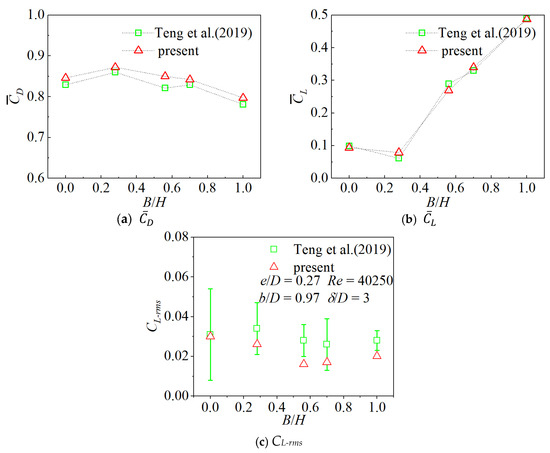
Figure 5.
Comparison of the hydrodynamic coefficients [22].
3. Results and Discussions
3.1. Computational Cases
As previously mentioned, under the given Reynolds number and boundary layer thickness, the primary parameters influencing the hydrodynamic coefficients of the cylinder with intermittent spanning arrangements are the gap ratio e/D, the total spanning ratio L/H, and the length of individual spanning l/D, where e/D takes values of 0.1, 0.2, and 0.3; the total spanning ratios take values of 0, 0.25, 0.50, 0.5, and 1; and the lengths of the single spanning l/D take values of 0, 8.7, and the intermediate value between the two values. Specific details can be seen in Table 5. It should be noted that, due to the significant computational costs, additional cases were added or removed during the research process based on partial results obtained. These adjustments will be reflected in subsequent figures and analyses. For all computational cases in this study, the Reynolds number Re = 42,500, and the boundary layer thickness δ/D = 3.

Table 5.
Computational cases.
3.2. Hydrodynamic Coefficients
For the cylinder with intermittent spanwise arrangements, Tong et al. [16] proposed the predictive formulas for hydrodynamic coefficients (1) and (2). To quantify the difference between the numerical results in this work and the predicted results established by Tong et al. [16] the parameters of relative errors ηD and ηL are used for representation, with the calculation formulas as shown in Equations (23) and (24):
where ηD and ηL are the parameters of relative errors between the mean drag coefficient obtained from numerical simulations and the corresponding empirical formula predictions for the lift coefficient . and are the time-averaged drag coefficients and time-averaged lift coefficients predicted by Equations (1) and (2), respectively.
To quantify force on the spanning sections and non-spanning sections, the drag force coefficient and lift force coefficient of non-span sections and a single non-span sections in Formulas (25) and (26) are calculated as follows:
where CD,S and CL,S represent the drag coefficient and lift coefficient of the spanning section, respectively. CD,NS and CL,NS represent the drag coefficient and lift coefficient of the non-spanning section, respectively. Similarly to Equation (12), FD,S and FL,S are the drag force and lift force acting on spanning section of cylinder, while FD,NS and FL,NS are the drag force and lift force acting on non-spanning section of cylinder, respectively.
3.2.1. Mean Drag Coefficient and Mean Lift Coefficient
The parameter of relative error ηD of the drag coefficient for multiple spanning cylinders varies with l/D is shown in Figure 6. It can be observed that when l/D ≤ 1, the relative error of the drag coefficient fluctuates dramatically with l/D; when l/D > 1, as l/D increases, the overall trend of ηD decreases gradually. In addition, for all cases in this work, it can be observed that the value of ηD is less than 5%, and under higher l/D, ηD even remains below 3%. It indicates that the empirical force prediction formula proposed by Tong et al. [16] can effectively predict the average drag coefficient for multiple spanning cylinders.
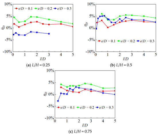
Figure 6.
Variation curves of ηD with l/D.
Figure 7 shows the variation in the relative error parameter of the mean lift coefficient ηL with l/D under different L/H conditions. It can be seen that when L/H = 0.25, ηL decreases gradually, then it increases at L/H = 0.5, and tends to stabilize. In most l/D cases, ηL is less than 5%. When L/H = 0.5 and 0.75, the results indicate that there is a significant deviation between the mean lift coefficients obtained through numerical simulations and the predicted results from the empirical formula proposed by Tong et al. [16]. Specifically, as l/D increases, the parameter of relative error ηL shows a decreasing trend. Furthermore, the results in Figure 7 demonstrate that the empirical prediction formula established by Tong et al. [16] tends to overestimate the mean lift coefficient, especially for the cases with large L/H. When L/H = 0.5, the values of ηL are approximately confined within the range of −25% to 0%. However, when L/H = 0.75, the values of ηL exhibit significant fluctuations within the range of −60% to 0%. This suggests that under larger L/D conditions, the overestimation of the existing formula becomes more marked, leading to greater deviation from the actual results. The above results indicate that the empirical prediction formula from Tong et al. [16] is effective in predicting the lift coefficient for small L/H ratio cylinders, but it cannot accurately predict the forces on spanning cylinders with L/H ≥ 0.5; therefore, further study on the lift coefficients of multiple spanning cylinders with L/H ≥ 0.5 is necessary.
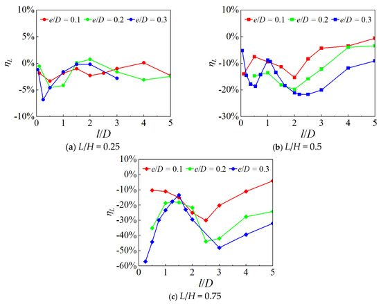
Figure 7.
Variation curves of ηL with l/D.
The lift coefficients of cylinders with a spanning ratio L/H = 0.5 is shown in Figure 8, where e/D ranges from 0.1 to 0.3. It is noted that and represent the time-averaged lift coefficients of the spanning cylindrical section, the non-spanning cylindrical section, and the entire cylinder, respectively. It is not difficult to observe that, under different e/D and l/D conditions, the time-averaged lift coefficient of the non-spanning section of cylinder is always greater than that of the spanning section. Meanwhile, the lift coefficient of the entire cylinder, serving as the average of the two parts, lies between the lift coefficient curves of the spanning and non-spanning section. This is primarily attributed to the fact that, beneath the non-spanning section of the cylinder, the flow is obstructed, resulting in higher pressure values. In contrast, beneath the spanning section of the cylinder, the flow is not impeded, leading to negative pressure values. In addition, it can be seen that when L/H = 0.5, the mean lift coefficient of all cylinders in the spanning section for e/D values of 0.1, 0.2, and 0.3 gradually decreases with the increase in l/D, stabilizing at approximately l/D > 2. This indicates that for l/D < 2, there is a significant interaction between the fluid in the spanning section and the non-spanning section. However, for l/D > 2, the influence of the spanning section on the non-spanning section weakens, and ultimately, the spanning section approaches a fully spanning condition. Additionally, it can be observed that the mean lift coefficient of the non-spanning section also gradually increases with the increase in l/D; similarly, the value tends to stabilize at l/D > 2.
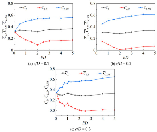
Figure 8.
Variation curves of , , with l/D, when L/H = 0.5.
Similarly, Figure 9 shows the dependence of the mean lift coefficients , and of the cylinder on l/D when L/H = 0.75, and e/D varies from 0.1 to 0.3. It can be observed that the variation in the mean lift coefficient for the non-spanning section follows the same trend as that when L/H = 0.5, gradually increasing with the increase in l/D and eventually stabilizing. For the spanning section of cylinder, when e/D is 0.1, the variation of aligns with the trend observed at L/H = 0.5, where it first decreases gradually, then increases slightly when l/D > 2.5, and finally stabilizes. When e/D is 0.2 and 0.3, the variation of is not significant when l/D < 1.5, and for l/D > 1.5, the trend is consistent with that at L/H = 0.5, which also gradually decreases and then rebounds after reaching a certain value of l/D, ultimately stabilizing. Compared to the cylinder with L/H = 0.50, the cylinder with L/H = 0.75, which has an increased spanning length, exhibits a lift coefficient of the entire cylinder and the spanning section that become closer in value, with a difference of approximately 0.1. This also implies that the blockage effect relatively weakens, particularly under larger e/D conditions, where the suppression effect near the wall diminishes, making this trend more marked.
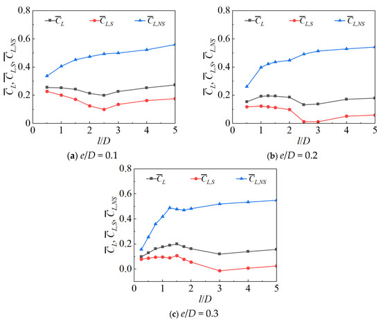
Figure 9.
Variation curves of , , with l/D, when L/H = 0.75.
To study the reasons for the variation of with l/D, the analysis of under all working conditions was conducted and shown in Figure 10. It can be seen that when the gap ratio e/D is fixed, the variation curves of with b/D for different L/H values are basically overlapping. This indicates that the spanning ratio L/H has little influence on the of the non-spanning section of the cylinder, and is mainly affected by the non-spanning section length b/D and the gap ratio e/D.
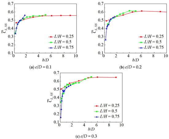
Figure 10.
Variation curves of , , with b/D.
3.2.2. Root Mean Square of Lift Coefficient and Root Mean Square of Drag Coefficient
This part focuses on the root mean square of lift coefficient CL-rms and drag coefficient CD-rms for multiple sections of cylinders. The analysis is conducted for the conditions of L/H = 0.5, e/D = 0.3, and l/D = 1. The results of CL-rms and CD-rms for each spanning section and non-spanning section are shown in Figure 11 and Figure 12. In the figures, S1–S5 represent the different spanning sections of the cylinder, while NS1-NS4 represent the different non-spanning sections; A represents the entire cylinder. It can be observed that the root mean square lift coefficient CL-rms of the spanning sections of cylinder is significantly greater than that of the non-spanning sections, while the root mean square drag coefficient CD-rms for both spanning and non-spanning sections is basically the same, indicating that the impact of the fluid in the gap on the drag coefficient is minimal. Additionally, it can be seen that the root mean square lift coefficient CL-rms and the drag coefficient CD-rms for each section of the cylinder, both spanning and non-spanning sections, are larger than the overall values of the cylinder. This is primarily due to the significant phase difference in vortex shedding across different cross-sections of the cylinder, which leads to mutual cancelation effects in the hydrodynamic coefficients during the integration process over the entire cylinder.
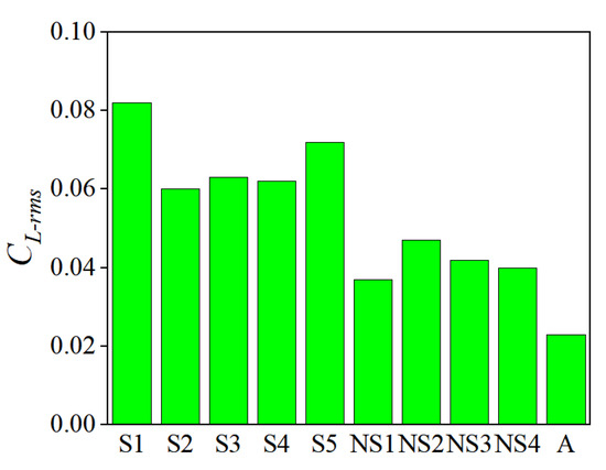
Figure 11.
CL-rms of each section, when L/H = 0.5, e/D = 0.3, l/D = 1.
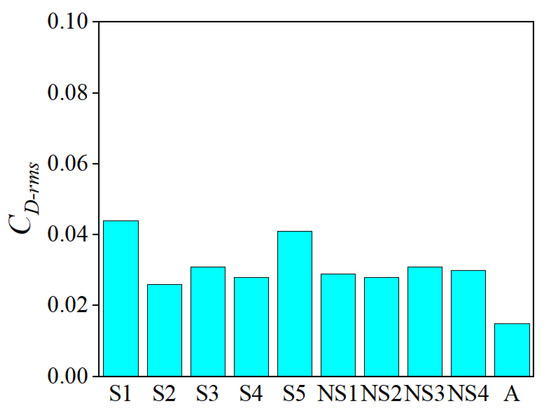
Figure 12.
CD-rms of each section, when L/H = 0.5, e/D = 0.3, l/D = 1.
3.2.3. Pressure Coefficient
It is well known that the forces acting on a cylinder are primarily influenced by the pressure distribution on its surface. The pressure coefficient Cp of a cylinder is discussed here. Figure 13 shows the distribution of the pressure coefficient Cp at the bottom of the cylinder when L/H = 0.5, e/D = 0.2, and l/D = 2. It can be observed that the middle part of the flow-approaching side of the non-spanning section of the cylinder exhibits higher pressure, with a region near the spanning section where the Cp gradually decreases toward the spanning section. In this study, the region where the pressure coefficient gradually decreases in the non-spanning span section is referred to as the transition section. In the spanning section, small negative pressure zones exist near both ends adjacent to the non-spanning sections, while a larger negative pressure zone is present closer to the mid-span region. This paper refers to these two negative pressure zones as low-pressure section A and low-pressure section B, respectively. Specifically, the low-pressure section A is primarily attributed to the deflection of fluid and vortices toward the non-spanning sections as flow passes the spanning section of the cylinder, whereas the low-pressure section B arises purely from the low-pressure region formed by vortices shed behind the spanning cylinder, analogous to the pressure distribution observed in an isolated cylinder.

Figure 13.
Cp at cylinder bottom for l/D = 1, e/D = 0.3, L/H = 0.75.
In order to investigate the variation in the lift coefficient of the non-spanning cylindrical sections with l/D, the pressure coefficient Cp of non-spanning cylindrical sections was analyzed under the conditions of e/D = 0.3, L/H = 0.5, and l/D = 0.5, 2, and 3. As shown in Figure 14, it can be observed that when e/D = 0.5, the high-pressure section in the middle of the non-spanning cylindrical sections is relatively low, while the transitional sections occupies a larger proportion. As l/D increases, although the range of the transitional sections does not show significant changes, its relative proportion gradually decreases, which leads to the gradual increase in the of the non-spanning cylindrical sections with the increase in l/D.
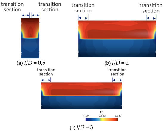
Figure 14.
Cp at bottom of non-spanning sections for e/D = 0.3, L/H = 0.5.
In addition, in order to study the variation in the lift coefficient of the cylindrical spanning section with l/D, for the cases of e/D = 0.2, L/H = 0.5, and l/D = 0.5, 2, 3, as well as e/D = 0.3, L/H = 0.5, and l/D = 0.5, 1.5, 3, the distribution of the bottom pressure coefficient Cp of the cylindrical spanning section was shown in Figure 15 and Figure 16. It can be seen that when L/H = 0.5 and e/D = 0.2, as l/D increases from 0.5 to 2, the low-pressure section of the spanning cylinder gradually expands, resulting in a decrease in ; when l/D increases from 2 to 3, the range of low-pressure section B no longer expands, which leads to a decrease in the proportion of low-pressure section B, thus increases; when L/H = 0.75 and e/D = 0.3, as l/D increases from 0.5 to 1.5, the Cp of low-pressure section A decreases and the range of low-pressure section B is relatively small, resulting in little influence on for the cylindrical spanning sections; as l/D increases from 1.5 to 3, the range of low-pressure section B expands, ultimately leading to a decrease in .
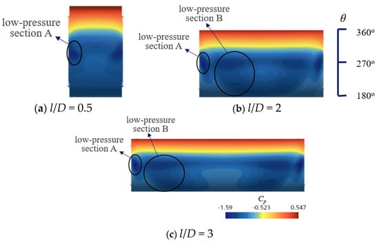
Figure 15.
Cp at bottom of non-spanning sections for e/D = 0.2, L/H = 0.5.
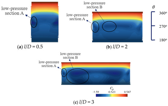
Figure 16.
Cp at bottom of non-spanning sections for e/D = 0.3, L/H = 0.75.
3.3. Characteristics of Flow Field
Figure 17 shows the time-averaged streamline cross-section when the gap ratio e/D = 0.3 for a completely spanning cylinder without blockage. It can be found that when the fluid flows past the cylinder, due to the presence of viscosity and reverse pressure gradient, the boundary layer separates from the surface of the cylinder, forming two vortices behind the cylinder. To facilitate a clear and intuitive comparison of the blockage effect on the flow field, Figure 18 depicts the time-averaged streamline results for a completely blocked cylinder at e/D = 0.3. It can be observed that the distribution of time-averaged streamlines at this time is significantly different from that of a completely spanning cylinder, with a larger-scale vortex forming behind the cylinder, while two smaller-scale vortices form upstream and downstream of the cylinder blockage.
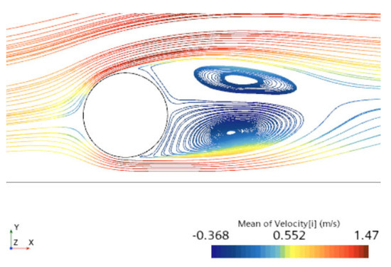
Figure 17.
Streamlines based on the averaged flow field of fully spanning cylinder with e/D = 0.3.
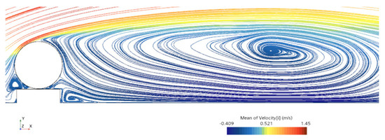
Figure 18.
Streamlines based on the averaged flow field of non-spanning cylinder with e/D = 0.3.
Figure 19 shows the time-averaged streamlines of a cylinder with l/D = 1, e/D = 0.3, and L/H = 0.5. It can be seen that when the fluid flows past the non-spanning section, due to the obstruction of the blockage at the lower part of the cylinder, the fluid is deflected towards the two sides of the spanning section. This results in a transitional area at the bottom of the non-spanning section where the pressure gradually decreases on both sides, and a low-pressure section A on both sides of the spanning section. When the fluid exits the gap, it is deflected towards the upper side and the blockage section of the cylinder, forming a three-dimensional vortex. The time-averaged streamline diagram for a cylinder with l/D = 1, e/D = 0.3, and L/H = 0.75 is shown in Figure 20. It can be found that the vortex is concentrated behind the cylinder, extending less towards the non-spanning section, and the rear vortex is more similar to a two-dimensional vortex. Figure 21 shows the time-averaged streamlines for l/D = 0.1, e/D = 0.3, and L/H = 0.75. It can be observed that after the fluid exits the gap, it flows perpendicular to the direction of the cylinder, forming two vortices behind, with larger scales in the downstream direction of the vortices.
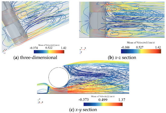
Figure 19.
Streamlines based on the averaged flow field at l/D = 1, e/D = 0.3, L/H = 0.5.
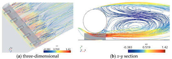
Figure 20.
Streamlines based on the averaged flow field at l/D = 1, e/D = 0.3, L/H = 0.75.
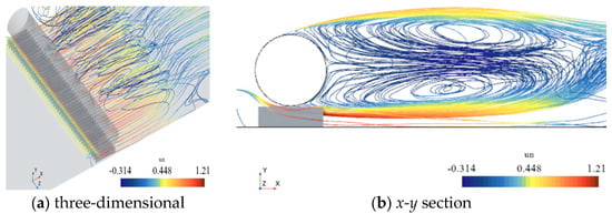
Figure 21.
Streamlines based on the averaged flow field at l/D = 0.1, e/D = 0.3, L/H = 0.75.
In addition, the results presented by the streamline in Figure 19 are consistent with the results of the pressure distribution described above. For a fixed e/D and L/H, as b/D increases, the proportion of flow deflected from the spanning section to the non-spanning section decreases. This consequently diminishes the relative proportion of the transitional section, ultimately leading to a decrease in . When L/H = 0.5 and e/D = 0.2, as l/D increases from 0.5 to 2, the gap beneath the cylinder expands. This allows more complete development of vortices behind the cylinder, leading to an expansion of the low-pressure section B and consequently a decrease in . As l/D further increases from 2 to 3, the extent of low-pressure section B ceases to expand. This reduction in the relative proportion of low-pressure section B ultimately results in an increase in .
4. Conclusions
The large eddy simulation method is used in this work to study the force characteristics and flow field distribution of circular cylinder with intermittent spanwise arrangements. The applicability of the hydrodynamic coefficient prediction formula for spanning cylinders proposed by Tong et al. [16] under the condition of a continuously varying spanning length l/D is explored. The main conclusions of this work are as follows:
The effect of the individual spanning length l/D on the time-averaged drag coefficient of uniformly spanning cylinders is minimal. The empirical formula proposed by Tong et al. [16] can accurately predict the drag coefficient of spanning cylinders under different uniform l/D ratios. For the lift coefficient, when the spanning ratio is small, such as L/H = 0.25, the effect of the single spanning length l/D on the lift coefficient of a uniform spanning cylinder is negligible; the empirical formula by Tong et al. [15,16] can also predict the hydrodynamic coefficients for cylinders well. However, when L/H ≥ 0.5, the effect of the single spanning length l/D on the lift coefficient of a cylinder is significant, and the previous empirical formulas cannot provide accurate predictions.
In addition, further research demonstrates that the total spanning ratio L/H has little influence on the of the non-spanning section of cylinder, and is mainly affected by the non-spanning section length b/D and the gap ratio e/D. Specifically, the lift coefficient of the non-spanning sections of the cylinder gradually increases with the increase in the single non-spanning length b/D. Flow visualization results show that it is mainly due to the fluid being deflected to the sides of the non-spanning sections after passing through the gap of the spanning section, creating a transitional region on both sides of the non-spanning section where the pressure gradually decreases. As b/D increases, the proportion of the transitional region decreases, resulting in an increase in for the non-spanning sections of the cylinder.
Author Contributions
Conceptualization, S.Y. and E.Z.; methodology, S.Y. and Y.W.; software, S.Y.; validation, S.Y. and E.Z.; formal analysis, S.Y., E.Z. and Y.W.; investigation, S.Y.; resources, Y.W.; data curation, E.Z.; writing—original draft preparation, S.Y., E.Z. and Z.J.; writing—review and editing, S.Y., Z.J., S.H. and G.T.; visualization, Z.J. and S.H.; supervision, Z.J., S.H. and G.T.; All authors have read and agreed to the published version of the manuscript.
Funding
The author Guoqiang Tang would like to acknowledge the support from the National Nature Science Foundation of China (Grant No. 52371262).
Data Availability Statement
All data generated or analyzed during this study are included in this published article. Additional data are available from the corresponding author upon reasonable request.
Conflicts of Interest
Songsong Yu, Erxian Zeng and Yadong Wang are employed by the Central Southern China Electric Power Design Institute Co., Ltd. of China Power Engineering Consulting Group. The remaining authors declare that the research was conducted in the absence of any commercial or financial relationships that could be construed as a potential conflict of interest.
Abbreviations
The following abbreviations are used in this manuscript:
| LES | Large eddy simulation |
References
- Williamson, C.H.K. Vortex dynamics in the cylinder wake. Annu. Rev. Fluid Mech. 1996, 28, 477–539. [Google Scholar] [CrossRef]
- Williamson, C.H.K. Defining a universal and continuous Strouhal–Reynolds number relationship for the laminar vortex shedding of a circular cylinder. Phys. Fluids 1988, 31, 2742–2744. [Google Scholar] [CrossRef]
- Williamson, C.H.K. The existence of two stages in the transition to three-dimensionality of a cylinder wake. Phys. Fluids 1988, 31, 3165–3168. [Google Scholar] [CrossRef]
- Wu, J.; Sheridan, J.; Welsh, M.C.; Hourigan, K. Three-dimensional vortex structures in a cylinder wake. J. Fluid Mech. 1996, 312, 201–222. [Google Scholar] [CrossRef]
- Bearman, P.W.; Zdravkovich, M.M. Flow around a circular cylinder near a plane boundary. J. Fluid Mech. 1978, 89, 33–47. [Google Scholar] [CrossRef]
- Zdravkovich, M.M. Forces on a circular cylinder near a plane wall. Appl. Ocean Res. 1985, 7, 197–201. [Google Scholar] [CrossRef]
- Lei, C.; Cheng, L.; Kavanagh, K. Re-examination of the effect of a plane boundary on force and vortex shedding of a circular cylinder. J. Wind Eng. Ind. Aerodyn. 1999, 80, 263–286. [Google Scholar] [CrossRef]
- Roshko, A.; Steinolfson, A.; Chattoorgoon, V. Flow forces on a cylinder near a wall or near another cylinder. J. Fluid Mech. 1975, 15, 1–3. [Google Scholar]
- Sumer, B.M.; Fredsøe, J. Flow around a cylinder in steady current. In Hydrodynamics Around Cylindrical Structures (Revised Ed.); World Scientific: Singapore, 2006; pp. 1–35. [Google Scholar]
- Ronold, K.O. A probabilistic approach to the lengths of free pipeline spannings. Appl. Ocean Res. 1995, 17, 225–232. [Google Scholar] [CrossRef]
- Buresti, G.; Lanciotti, A. Vortex shedding from smooth and roughened cylinders in cross-flow near a plane surface. Aeronaut. Q. 1979, 30, 305–321. [Google Scholar] [CrossRef]
- Griffiths, T.; Shen, W.; Xu, M.; Leggoe, J. Comparison of recent parametric trenched and partially embedded/spanning pipelines with DNV-RP-F109 load reduction design curves. In Proceedings of the OMAE2012, Rio de Janeiro, Brazil, 1–6 July 2012. [Google Scholar]
- Sollund, H.A.; Vedeld, K.; Hellesland, J.; Fyrileiv, O. Dynamic response of multi-span offshore pipelines. Mar. Struct. 2014, 39, 174–197. [Google Scholar] [CrossRef]
- Teng, Y.; Griffiths, T.; Tang, G.; An, H.; Draper, S.; Cheng, L.; Mohr, H. Peak force coefficients on small-diameter spanning pipelines under waves. Coast. Eng. 2022, 177, 104189. [Google Scholar] [CrossRef]
- Tong, F.; Cheng, L. Numerical study on steady flow around a pipeline laid on seabed with gaps. In Proceedings of the ISOPE PACOMS, Gold Coast, Australia, 4–7 October 2016. [Google Scholar]
- Tong, F.; Cheng, L.; An, H.; Griffiths, T. The hydrodynamic forces on a circular cylinder in proximity to a wall with intermittent contact in steady current. Ocean Eng. 2017, 146, 424–433. [Google Scholar] [CrossRef]
- Rhie, C.M.; Chow, W.L. A numerical study of the turbulent flow past an isolated airfoil with trailing edge separation. In Proceedings of the 3rd AIAA/ASME Joint Thermophysics and Heat Transfer Conference, St. Louis, MO, USA, 7–11 June 1982. [Google Scholar]
- Germano, M.; Piomelli, U.; Moin, P.; Cabot, W.H. A dynamic subgrid-scale eddy viscosity model. Phys. Fluids 1998, 3, 1760–1765. [Google Scholar] [CrossRef]
- Breuer, M. Large eddy simulation of the subcritical flow past a circular cylinder: Numerical and modeling aspects. Int. J. Numer. Methods Fluids 1998, 28, 1281–1302. [Google Scholar] [CrossRef]
- Vreman, B.; Geurts, B.; Kuerten, H. Realizability conditions for the turbulent stress tensor in large-eddy simulation. J. Fluid Mech. 1994, 278, 351–362. [Google Scholar] [CrossRef]
- Balaras, E.; Benocci, C.; Piomelli, U. Two-layer approximate boundary conditions for large-eddy simulations. AIAA J. 1996, 34, 1111–1119. [Google Scholar] [CrossRef]
- Teng, Y.; Cheng, L.; An, H.; Tong, F.; Xiong, Z. Hydrodynamic forces on intermittently spanning pipelines in steady currents. In Proceedings of the ASME OMAE, Glasgow, UK, 9–14 June 2019; pp. 9–14. [Google Scholar]
- Khan, N.B.; Ibrahim, Z.; Badarudin, A.; Jameel, M.; Javed, M.F. Numerical investigation of flow around cylinder at Reynolds number=3900 with large eddy simulation technique: Effect of spanwise length and mesh resolution. Proc. Inst. Mech. Eng. M J. Eng. Marit. Environ. 2019, 233, 417–427. [Google Scholar] [CrossRef]
- Behr, M.; Hastreiter, D.; Mittal, S.; Tezduyar, T.E. Incompressible flow past a circular cylinder: Dependence of the computed flow field on the location of the lateral boundaries. Comput. Methods Appl. Mech. Eng. 1995, 123, 309–316. [Google Scholar] [CrossRef]
Disclaimer/Publisher’s Note: The statements, opinions and data contained in all publications are solely those of the individual author(s) and contributor(s) and not of MDPI and/or the editor(s). MDPI and/or the editor(s) disclaim responsibility for any injury to people or property resulting from any ideas, methods, instructions or products referred to in the content. |
© 2025 by the authors. Licensee MDPI, Basel, Switzerland. This article is an open access article distributed under the terms and conditions of the Creative Commons Attribution (CC BY) license (https://creativecommons.org/licenses/by/4.0/).