Article

Machine Learning-Based Spatiotemporal Acid Mine Drainage Prediction Using Geological, Climate History, and Associated Water Quality Parameters

1
BGRIMM Technology Group Co., Ltd., Beijing 100160, China
2
Department of Civil Engineering, Institute of Geotechnical Engineering, Zhejiang University, Hangzhou 310058, China
*
Author to whom correspondence should be addressed.
Water 2025, 17(18), 2661; https://doi.org/10.3390/w17182661
Submission received: 16 July 2025 / Revised: 25 August 2025 / Accepted: 29 August 2025 / Published: 9 September 2025
(This article belongs to the Special Issue Water, Geohazards, and Artificial Intelligence, 2nd Edition)

Abstract

Acid mine drainage (AMD) poses significant environmental and health risks due to its high acidity and elevated metal and sulfate contents. Previous studies have primarily focused on short-term AMD monitoring, with limited attention paid to long-term, spatially resolved datasets and predictive modeling. In this 3.5-year study, six wells down-stream of a mine waste rock pile were monitored, and 132 sets of associated water quality (AWQ), geological (GEO), and climate history (CH) parameters were compiled to develop predictive models for Fe, Cu, and Zn concentrations. Random forest (RF), extreme gradient boosting (XGBoost), and support vector machine (SVM) algorithms were applied using different combinations of input variables. The combined AWQ-GEO-CH dataset achieved the best overall performance, with XGBoost yielding the highest R2 values for Fe (0.81) and Cu (0.77), and SVM performing best for Zn (0.94). CH variables, particularly precipitation and evaporation over 60-day periods, strongly influenced metal concentrations by driving hydrological and solute redistribution processes. AWQ parameters, especially F and S2−, were key predictors for Fe and Zn and ranked second for Cu, likely due to shared upstream sources and coupled geochemical processes such as FeF3 dissolution. The most impactful GEO factor was the installation of a vertical barrier, which reduced metal concentrations by 73–80%. These findings highlight the value of integrating multi-source datasets with ML for long-term AMD prediction and management.

1. Introduction

Mineral extraction activities have increased in recent years due to booming industries related to global manufacturing, electric vehicles, and renewable energy [1,2]. These activities result in massive deposits of mine waste rocks that are low in ore content, but highly conducive to acid mine drainage (AMD) upon exposure to moisture and oxygen [3,4]. AMD formation is primarily driven by oxidative reactions involving sulfide minerals, which produce sulfuric acid and dissolve various metal ions. AMD problems are exacerbated in open mine waste rock piles that are the major form of mine waste disposal in China, Australia, and many other countries [5,6]. In China, 52 billion tons of mine waste rocks have been aggregated and exposed to the air, such that AMD caused by pyrite (FeS2) oxidation poses a major environmental challenge [7,8]. Pyrite is common in metal mine waste rock and its exposure to air and water leads to oxidation and the generation of AMD that is typically characterized by low pH (2–4) and elevated concentrations of metals and sulfate (SO42−) [6,7]. AMD poses significant threats to natural environments and human health in many countries via water and soil pollution, in addition to contamination of food chains. Consequently, technologies that mitigate environmental pollution issues related to mining operations, and particularly AMD, are of interest to mine owners, policymakers, and other stakeholders.
Vertical barriers that comprise low permeability materials such as cement-based grouts or bentonite (as in the geosynthetic liner, GCL) are effective in containing underground AMD from spreading [9,10,11,12,13]. For example, Li et al. [14] used vertical cement curtain grouting to block AMD pathways in a karst coalfield while integrating source isolation with lime neutralization and wetland treatment. These strategies led to reduction in Fe concentrations to below 0.03 mg/L and restoration of spring water quality to regulatory standards within two years. Similarly, Wu et al., [11] developed an integrated AMD control system that combined grouting-based source isolation with vertical curtain grouting and wetlands to achieve compliant effluent with a pH of 6.9–7.9 and Fe concentrations < 0.1 mg/L within half a year. Despite promising effective short-term results, comprehensive long-term monitoring and prediction remain limited, primarily due to challenges associated with deploying expensive and labor-intensive borehole sampling analyses over relatively large areas. An effective method to evaluate the spatial extent of AMD contamination over entire mine waste rock sites over longer timespans (e.g., years) is therefore urgently needed [7,15].
Machine learning (ML) has been used to predict heavy metal concentrations in AMD via efficient modeling and forecasting of multiple variables, including nonlinear and heterogeneous datasets from multiple sources. For example, Rooki et al. [16] used an artificial neural network (ANN) that included dataset inputs of pH and sulfate concentrations to predict heavy metal concentrations (e.g., of Cu, Mn, and Zn) in the Sarcheshmeh copper mine of Iran, consequently achieving a coefficient of determination (R2) > 0.9. In addition, Kabuba and Maliehe [17] demonstrated that a three-layer backpropagation (BP) neural network trained with the Levenberg-Marquardt algorithm yielded exceptional prediction (R2 = 0.99) of Cu, Fe, Mn, and Zn concentrations in a South African mine, while incorporating pH, SO 4 2 , and total dissolved solids as inputs. Trifi et al. [18] compared the effectiveness of random forest (RF), support vector machine (SVM), and ANN models for predicting Zn, Pb, Mn, Cu, Cd, and Fe concentrations in tailing ponds and surrounding soils at the Sidi-Driss mining site in Tunisia. Mineral composition, grain size, SO 4 2 , and sulfur (S) content were incorporated into the models, revealing that the RF model was most predictive (R2 values of 0.575, 0.752, and 0.597 for Fe, Cu, and Zn, respectively). Nevertheless, the reviewed literature generally lacked a detailed exploration of the interpretability of ML models applied to AMD contamination prediction, particularly regarding the identification of key influential parameters that could provide insights into source identification, reaction and transport mechanisms, and guidance for pollution prevention.
The SHapley Additive exPlanations (SHAP) method is grounded in cooperative game theory and quantifies the contribution of each input feature toward model predictions, consequently offering an intuitive and interpretable perspective to assess feature impacts. Li et al. [19] applied SHAP to an XGBoost model to identify variables that most influenced soil Cu release, including agricultural irrigation volume, organic matter content, and mine drainage flow, ultimately identifying agricultural irrigation as the dominant factor. In addition, Ref. [20] identified temperature, total dissolved solids, and iron concentrations as the most important variables for predicting sulfate concentration levels, wherein strong iron-sulfate correlations implicated the presence of dissolved pyrite. Zhao et al. [21] used SHAP to interpret six ML models that predicted heavy metal cation adsorption, including variants of RF, gradient boosted RF, extra trees, gradient boosting decision tree, extreme gradient boosting, LightGBM, and categorical boosting models. The analyses identified the hydrolysis and solubility product constants as the most influential parameters for adsorption, while specific surface area, solid concentration, background ionic strength, adsorption temperature, adsorption time, pH, atmospheric CO2, and background ion species were less important. Thus, SHAP analysis provides feature interpretation for mainstream “black-box” ML models that bridge the gap between predictive performance and mechanistic understanding in environmental applications.
Geological (GEO), climate history (CH), and associated water quality (AWQ) parameter sets are the most influential for AMD contamination prediction. Current machine learning algorithms often only consider partial parameters, due to the time and labor-intensive field measurements that are prohibitive and which may undermine or even omit dominant factors. GEO, CH, and AWQ input parameters are also generally the most accessible for gathering data (in the indicated order), although prior studies do not necessarily follow this sequence. In addition, climate parameters including precipitation, evaporation, temperature, and humidity are physically and tightly related to AMD generation and transport. Indeed, climatic factors regulate the spatiotemporal evolution of AMD in groundwater by modulating water fluxes, thermal regimes, and geochemical conditions, thereby influencing dilution/concentration dynamics and redox-mediated metal precipitation, in addition to hydrodynamic transport and retention processes [22,23,24]. Nordstrom [22] reported that extended drought and evaporation facilitate salt crust and secondary mineral formation in tailings, consequently concentrating contaminants that are subsequently mobilized during initial rainfall via a pronounced “first flush” that enhances infiltration into the ground. Liu et al., [24] confirmed that precipitation significantly facilitates the migration and accumulation of contaminants from AMD into groundwater by enhancing pyrite oxidation and heavy metal leaching. However, incorporating climate history into predictive models remains a significant challenge, particularly for defining appropriate time windows in water rebalance restoration, solute redistribution, and legacy effects. Consequently, climate history has not been adequately integrated into most AMD-related groundwater studies.
Despite advances in AMD prediction using machine learning, several critical gaps remain. First, most studies rely on short-term or site-specific monitoring, which limits their ability to provide a full understanding of temporal variability and extreme events, as they fail to capture multi-year trends. Second, while geological, climate, and water quality factors are known to influence AMD dynamics, they have rarely been evaluated together within an integrated, comparative framework. Third, the role of climate history, particularly the optimal time windows for precipitation and evaporation effects, remains poorly quantified, despite its strong physical link to AMD generation and transport [22,23]. Finally, the connections between machine learning predictions and physical processes are often overlooked, restricting the ability to identify dominant environmental drivers and translate findings into practical pollution control strategies.
To bridge these gaps, the aim of this study is to identify key factors that influence AMD contamination downstream of a full-scale waste rock site through machine learning algorithms and the SHAP method. Specifically, the objectives are to: (1) conduct a 3.5-year groundwater quality monitoring study at six wells downstream of an acidic water reservoir, collect associated water quality (AWQ) data, and integrate geological (GEO) and climate history (CH) data to train the ML models; (2) develop and compare the performance of RF, XGBoost, and SVM models in predicting Fe, Cu, and Zn concentrations using different combinations of AWQ, GEO, and CH input parameters; and (3) apply SHAP analysis to quantify the relative importance of each parameter set and identify key processes governing AMD contamination. By connecting predictive performance with geophysical processes, this study aims to provide a robust and interpretable framework for AMD risk assessment and management.

2. Materials and Methods

2.1. Study Area

The acidic water reservoir is located at the Dexing Copper Mine (which is situated in Shangrao City, Jiangxi Province, China) that covers an area of approximately 4 km2, and which was constructed in a valley and enclosed by a concrete gravity dam that was designed for a 20-year precipitation return period. The dam exhibited a crest elevation of +146.50 m, a width of 5.0 m, and a length of 172.03 m while exhibiting a base width of 35.65 m, a maximum height of 43.5 m, and a normal water level elevation of 144.00 m. The reservoir area features Quaternary phreatophyte, alluvial-proluvial, and eluvial-diluvial deposits, as well as Sinian phyllite, with mud interlayers along foliation planes. The respective thicknesses of the layers were 0.20–0.50 m, 1.70–5.60 m, 1.60–7.20 m, 15.3–43.5 m, and 0.60–0.90 m. The site exhibits a subtropical humid monsoon climate, with an annual average temperature of 17.4 °C, and an annual precipitation of 1930 mm. Groundwater in the area is predominantly Quaternary pore water and bedrock fissure water. The former is recharged by river infiltration, precipitation, and fissure flow, exhibiting pronounced seasonal fluctuations. The latter is topographically controlled, recharged by surface runoff and precipitation, and typically discharges via springs that feed nearby rivers. Six monitoring wells (W01 through W06) were installed downstream of the reservoir in a zig-zag pattern to assess long-term groundwater quality impacts following reservoir construction (Figure 1). A vertical barrier was installed at the downstream end of the reservoir on 1 January 2021 using low-permeability materials that aimed to reduce possible leakage (Figure 1).

2.2. Data Collection

A total of 132 groundwater samples were collected from six monitoring wells (W01–W06 in Figure 1), which are arranged approximately linearly at distances of 299, 432, 575, 855, 1219, and 1562 m from the reservoir center. Each well was sampled at two-month intervals 22 times from 1 February 2019 to 1 August 2022. Sampling procedures were: Prior to sampling, the wells were purged until temperature, pH, and conductivity readings stabilized, and the out-flow appeared clear. For volatile organic compounds (VOCs), water samples were collected in pre-cleaned, airtight containers without headspace at a controlled flow rate of 0.2–0.5 L/min, whereas other parameters were sampled at a flow rate of less than 1 L/min. All sampling containers were rinsed with the well water prior to collection (except for VOCs), and samples for different analytes, including semi-volatile organics, inorganic ions, trace metals, and microbiological and radiological indicators, were collected separately to avoid cross-contamination. After collection, the sample containers were immediately sealed, labeled, and stored at 4 °C until analysis. Samples were processed using standard protocols and analyzed using ICP-MS spectrometry (standard HJ 766-2015 [25]) to measure concentrations of Fe, Zn and Cu. The concentrations of six AWQ parameters, including F, S2−, pH, SO 4 2 , NH 4 + , and COD were also measured.
GEO parameters were also evaluated, including distance, permeability (k), barrier installation, and distribution coefficients (calculated in Text S1) for Fe, Cu, and Zn (Table 1). In addition, the embankment was fully completed on 1 January 2021; thus, its value is set to 0 before this date and 1 thereafter.
CH records were obtained from the China Meteorological Data Service Centre. At each sampling event, climate conditions over the preceding 0, 3, 7, 10, 20, 30 and 60 days were compiled, including cumulative precipitation and evaporation, in addition to average humidity and temperature. Evaporation (evap) was also estimated using the Penman equation as described below in Equation (1).
E T 0 = Δ R n + γ ρ a C p e s e a r a λ v ( Δ + γ ) × 86.4
R ns = k 1 C 100 86400
where E T 0 is evaporation, ρ a is the air density (kg/m3), e s is the saturated vapor pressure (Pa), e a is the actual vapor pressure (Pa), r a is the aerodynamic resistance (s/m), Δ is the slope of the saturated vapor pressure curve (Pa/K), λ v is the latent heat of vaporization (J/kg), and γ is the psychrometric constant (Pa/K), R n is the net shortwave radiation (W/m2), k = 0.066 and is the extraterrestrial radiation coefficient, C is the daily average total cloud cover (%), and 86,400 and 86.4 represent time-dimensional conversion factors.

2.3. Workflow for Heavy Metal Concentration Prediction

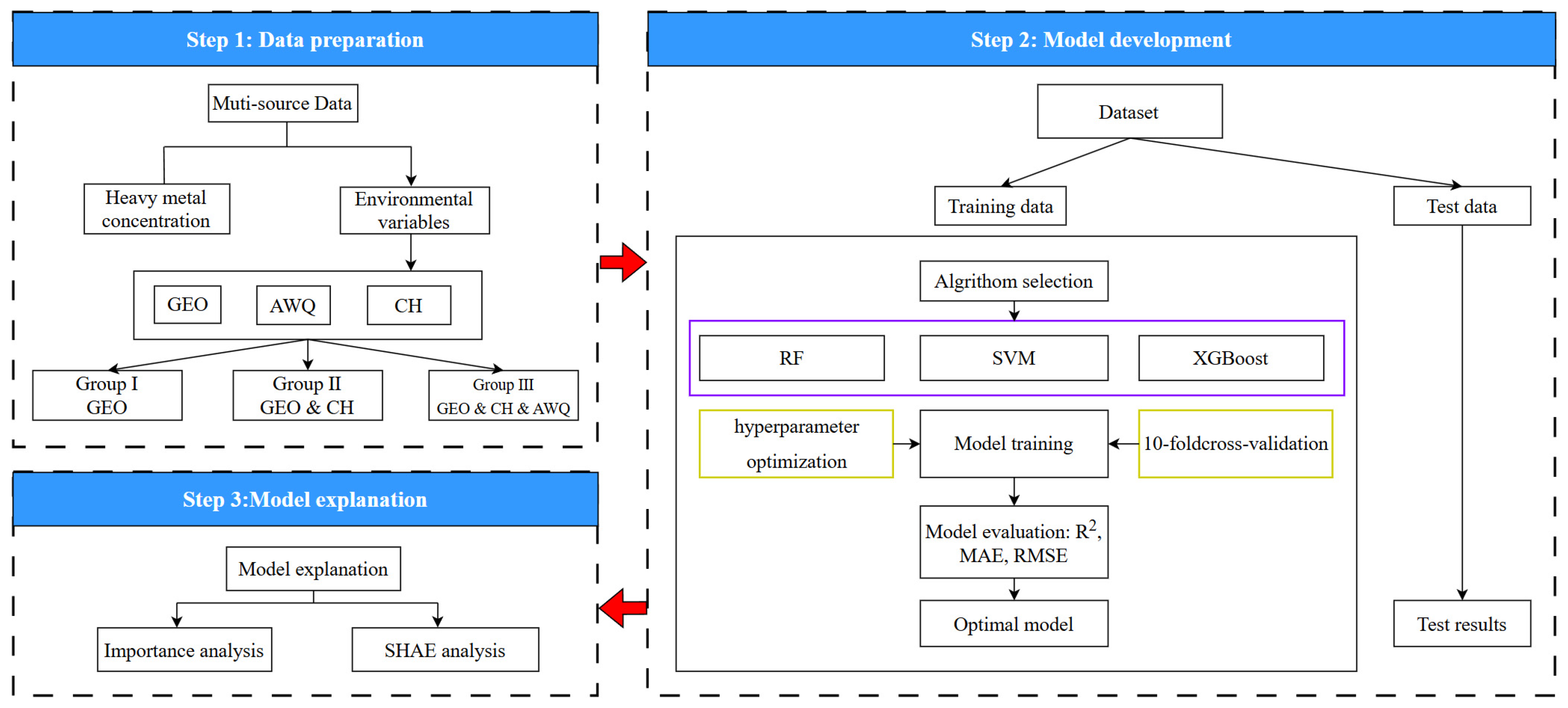
The workflow for predicting the concentration of heavy metals is shown in Figure 2, and it included three steps, i.e., data preparation, model development, and model explanation.

2.4. Methods

2.4.1. Data Segmentation

The dataset was randomly divided into training and test sets. Following the common practice in ML research, 80% of the data was assigned to the training set and 20% to the test set [26,27]. A 10-fold repeated cross-validation strategy was used during model training [26].

2.4.2. Model Selection

Three popular ML algorithms including RF, XGBoost, and SVM models were used to predict the three target metal concentrations. RF is an ensemble-based regression model that constructs multiple decision trees by bootstrapping samples. Final predictions are then obtained by averaging outputs from individual trees [28,29,30]. XGBoost is a gradient-boosted ensemble method that is optimized for computational efficiency and prediction accuracy. The method generates a series of regression trees, where each tree corrects the residuals of previous ones [31,32]. SVM for regression (also known as support vector regression, SVR), estimates a function within a specified error tolerance by fitting a hyperplane in high-dimensional space. A kernel function is also applied when linear relationships are insufficient [33,34].

2.4.3. Hyperparameter Optimization

To mitigate overfitting, hyperparameter optimization was conducted using the Optuna package. For the SVM model, the optimization space included parameters such as the kernel function type, regularization parameter C, kernel coefficient gamma, insensitive loss parameter epsilon, and polynomial kernel degree. In the case of the Random Forest and XGBoost models, the optimization space covered parameters that included the number of trees, maximum tree depth, and regularization strength. Through iterative processes of cross-validation and evaluation based on mean squared error (MSE) performance, the optimal hyperparameters were selected for each model (Table S1).

2.4.4. SHAP

SHAP is a model interpretation method grounded in cooperative game theory. Its fundamental principle is to evaluate the marginal contribution of each input feature across all possible feature subsets and compute a weighted average of these contributions to quantify the feature’s importance to the model’s predictions (see Text S2 for details).

2.4.5. Model Evaluation

To comprehensively quantify prediction error distributions and assess model fit, model performance was evaluated using the mean squared error (MSE), root mean squared error (RMSE), mean absolute error (MAE), the coefficient of determination (R2), and Willmott Index (WI).
All predictive analyses were performed on a workstation equipped with an Intel processor comprising 24 physical cores and 32 logical threads, as well as 63.76 GB of RAM. The computational environment was based on Python 3.11.5 (Anaconda distribution; build: MSC v.1916, 64-bit; AMD64 architecture).
M S E = 1 n i = 1 n ( y i y ^ i ) 2
R M S E = 1 n i = 1 n ( y i y ^ i ) 2
R 2 = 1 i = 1 n ( y i y ^ i ) 2 i = 1 n ( y i y ¯ ) 2
M A E = 1 n i = 1 n | y i y ^ i |
W I = 1 i = 1 n ( y i y ^ i ) 2 i = 1 n ( | y ^ i y ¯ | + | y i y ¯ | ) 2

3. Results and Discussion

3.1. Heavy Metal Concentration

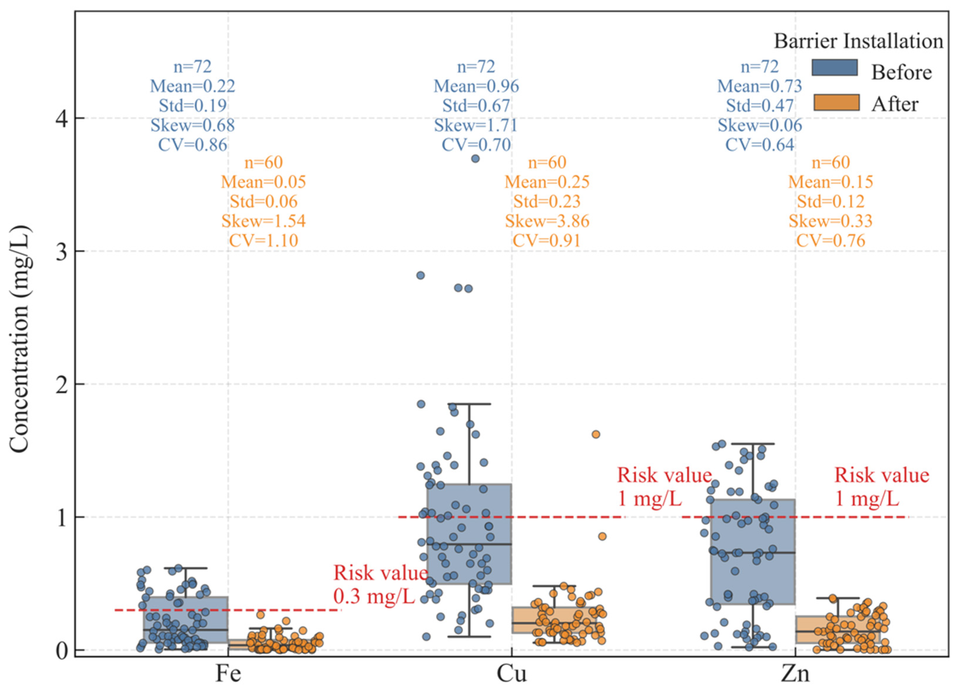
Groundwater samples were classified into two groups based on collection dates before and after the barrier’s installation on 1 January 2021 (Figure 3), to compare the concentrations of Fe, Zn, and Cu between the two periods (Figure 3). Before the barrier was established, 72 samples were collected, with mean concentration of Cu (0.96 mg/L) being the highest, followed by Zn (0.73 mg/L) and Fe (0.22 mg/L). The number of samples exceeding the quality standards for classification III groundwater (GB/T 14848-2017 [35]) was 22 for Fe (0.3 mg/L), 28 for Cu (1 mg/L), and 22 for Zn (1 mg/L). After the installation of the barrier, 61 samples were collected, and the mean heavy metal concentrations declined substantially: Cu to 0.25 mg/L, Zn to 0.15 mg/L, and Fe to 0.05 mg/L (Figure 3). Only one Cu sample exceeded the threshold, while Fe and Zn remained below their respective limits in all cases. This may indicate that, in addition to the upstream reservoir, other unidentified sources of Cu contamination exist. These findings demonstrate the barrier’s effectiveness in limiting heavy metal transportation and enhancing groundwater quality.
The coefficient of variation (CV), which serves a statistical measure of dispersion, exceeded 50% for Fe, Cu, and Zn, indicating pronounced spatial and temporal dispersion in their concentrations, regardless of the barrier installation status. This fluctuation is primarily driven by the regional hydrological cycle, which features three distinct periods: a wet season from March to July, contributing approximately 70% of the annual precipitation; a moderate-flow season from August to November; and a dry season from December to February. During the wet season, increased runoff enhances leaching processes and accelerates pollutant transport [36]. Skewness values increased for all three metals following barrier installation, which may have resulted from transitional effects during the implementation phase, as well as the use of a single reference date for separation, this, in turn, could have resulted in classification bias. Cu exhibited the highest skewness (3.86), suggesting a longer right tail and a higher likelihood of extreme concentrations.

3.2. Overall Prediction Performance

The performances of SVM, RF, and XGBoost model predictions of AMD were investigated using geological parameters (GEO), climate history parameters (CH), and associated water quality parameters (AWQ) (Table S1). For Fe concentration prediction, the SVM achieved the highest R2 with 0.64 on GEO, RF had the highest R2 of 0.73 on GEO & CH, and XGBoost exhibited the highest R2 of 0.805 on GEO & CH & AWQ. This suggests that SVM, RF and XGBoost have a similar performances on small datasets [37]. Generally, the SVM, RF, and XGBoost models exhibited greater predictions using input parameters in the order of GEO & CH & AWQ > GEO & CH > GEO. Thus, more input parameters yielded better predictions, partially due to the tree-based algorithms (RF and XGBoost) inherently performing feature selection [38]. During tree-building, the XGBoost algorithm selects features with the highest information gain to generate splits [39] that then allows the model to better handle nonlinear relationships between heavy metal cation concentrations and environmental covariates, including those parameterized in the GEO, CH, and AWQ inputs. In addition, the regularization mechanism of XGBoost contributes to lowering model variability, thereby reducing overfitting risks and strengthening performance with high-dimensional environmental variables (i.e., with the GEO, CH, and AWQ inputs) [40]. The two exceptions to the performance hierarchy are the flips of the SVM model that used GEO parameters alone and the SVM model that used GEO and CH parameters to predict Fe and Cu concentrations (Table S1). The latter likely resulted from SVM models being affected by collinearity among climate history variables. For example, obvious collinearity is observed among accumulated precipitation calculated over 0, 3, 7, 10, 20, 30, and 60 days. SVM algorithms attempt to identify a hyperplane with a maximum margin and are sensitive to redundant features and high-dimensional noise. These redundant features can distort distance metrics in feature space [41]. However, when the associated water quality parameters were added to the model, SVM model performance significantly improved, with R2 values increasing from 0.57 to 0.73. AWQ parameters, including pH and COD, in addition to the concentrations of fluoride and sulfide, are physically influenced by climate factors. For example, precipitation leads to dilution or enrichment and can thus also interact with geological parameters such as permeability (Figure S8) [42]. Overall, the intricate connections among the three sets of input parameters were effectively captured by the SVM model, resulting in accurate predictions of target metal concentrations.
The XGBoost algorithm incorporating all three sets of input parameters generated the best prediction for Fe (R2 = 0.805) concentrations, while the SVM algorithm and the RF algorithm generated the best prediction for Zn (R2 = 0.94) and Cu (R2 = 0.896) concentrations, respectively. Computational cost and time are important considerations when conducting practical model selection, and especially for engineering applications [43]. Training and testing times followed the order of SVM (7 min 7 s) < RF (23 min 9 s) < XGBoost (37 min 19 s). Based on prediction performance and time efficiency, the SVM model with three sets of input parameters was then selected for parametric sensitivity analysis.

3.3. Accuracy of Fe, Cu, and Zn Concentration Predictions

When considering only the GEO parameters, the predicted concentrations of Fe, Zn, and Cu exhibited R2 values of 0.798 (Figure S1), 0.941 (Figure S2), and 0.877 (Figure S3), respectively, indicating acceptable predictive performance. The addition of CH parameters led to predicted R2 values for Fe, Cu, and Zn concentrations increasing to 0.830, 0.916, and 0.958, respectively. Moreover, although 38 environmental variables selected based on GEO & CH & AWQ were directly or indirectly associated with the prediction of heavy metal cations, other environmental variables beyond those included in the models, that might influence cation exchange, were not accounted for. For example, total dissolved solids (TDS) and electrical conductivity (EC) have been demonstrated to be a significant contributor to Fe cations in the river near the Sarcheshmeh copper mine [44]. Without such variables from the model, which could have curtailed its predictive accuracy for Fe. However, it is encouraging to note that the predictive accuracy in our study for Fe, Zn, and Cu on GEO & CH was superior to that reported by Trifi et al., [18], where the R2 values for Fe, Cu, and Zn concentrations in an AMD environment were 0.575, 0.752, and 0.597, respectively. Trifi et al., [18] used RF modeling with 11 mineralogical composition parameters, in addition to other input parameters including five physicochemical parameters (S2−, SO 4 2 , pH, electrical conductivity, and cation exchange capacity) and grain size distribution. The improved performance observed in this study is primarily attributed to the addition of CH parameters. The addition of AWQ input parameters led to further prediction improvement, with R2 values of 0.866 (Fe), 0.973 (Zn), and 0.904 (Cu) observed. These observations underscore the importance of considering aquatic chemical speciation, including both chemically non-reactive ions (e.g., F) and reactive ions (e.g., S2−), as further discussed in later sections.
While the models exhibited improved performance with the inclusion of additional predictors, as reflected in the higher R2 and lower RMSE values for the training datasets, there was a potential risk of overfitting, particularly for the Fe and Cu models (Figures S1 and S2). As the number of predictors increased, we found that the training R2 values rose more sharply than the test R2 values, indicating that the models may have been capturing noise in the training data. This suggests that the models, particularly for Fe and Cu, may have been overly tailored to the training set, reducing their generalizability to new data. Such behavior is a common indication of over-fitting, wherein which the model becomes too complex and fits the peculiarities of the training data instead of capturing the underlying trend. In contrast, the Zn models demonstrated a more balanced performance, with less discrepancy between the training and test R2 values, suggesting that these models are less prone to overfitting (Figure S3). These observations warrant further consideration, as they highlight the need for careful model validation when using multiple predictors. Future work should explore methods such as regularization or feature selection to mitigate the risk of overfitting while maintaining or improving predictive accuracy.

3.4. Parametric Analysis of Fe Concentration Predictions

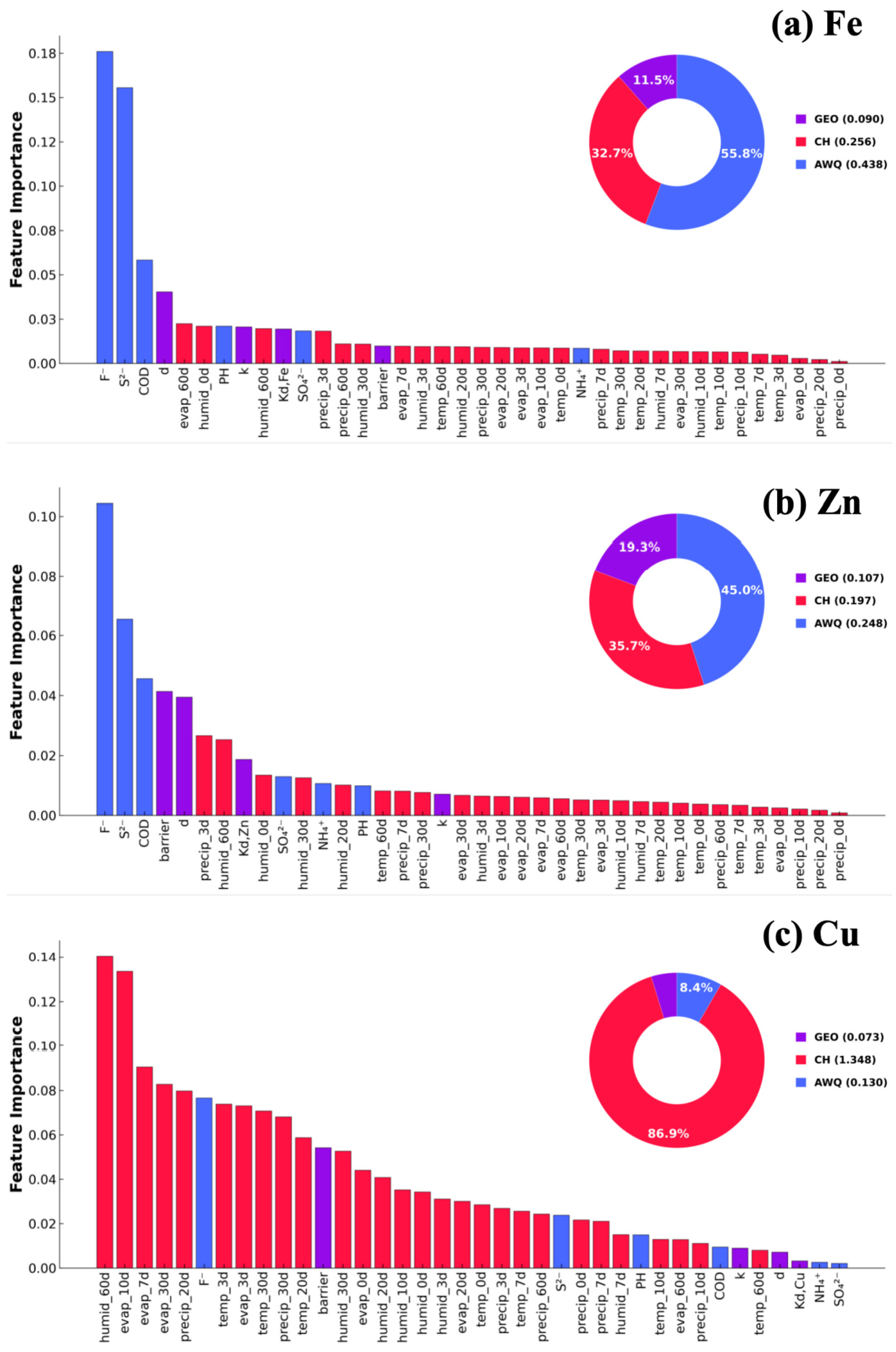
An analysis of the relative importance of model parameters based on the SHAP method was conducted (Figure 4). AWQ parameters, and particularly F and S2− concentrations, dominantly contributed to Fe concentration predictions, with accumulated contribution weights (ACW) of 55.8% (Figure 4a). F from CaF2 is commonly found in mine waste piles [19], while sulfide in forms such as Cu2S, Cu5FeS4, and CuFeS2 is also commonly observed in mine waste rocks [24,45]. Fluoride and sulfide are transported downstream with iron cations to the six observation wells, with all three elements subject to the same dilution or concentration processes induced by precipitation or evaporation. Furthermore, the coexistence of Fe3+ and F is conducive to the formation of ferric fluoride (FeF3), whose high solubility (0.033 g/L at 25 °C; [46] facilitates hydrolysis reactions, thereby promoting the release and retention of both Fe3+ and F. Consequently, Fe3+ and F concentrations were positively correlated (ACW of 22.4%) due to the shared reservoir source, downstream transportation pathway, and hydrolysis reactions. S2− is not as stable as F in mines and experiences oxidation and surface complexation. Consequently, S2− also showed a positive contribution (ACW of 19.8%) to Fe prediction, likely due to their shared source and transport pathway, although this contribution was weaker than that between F and Fe3+, primarily due to greater reactivity of S2−. The contribution of pH to Fe cations was limited (ACW of 2.7%), owing to the weak acidic to neutral pH environment (4.38–7.38).
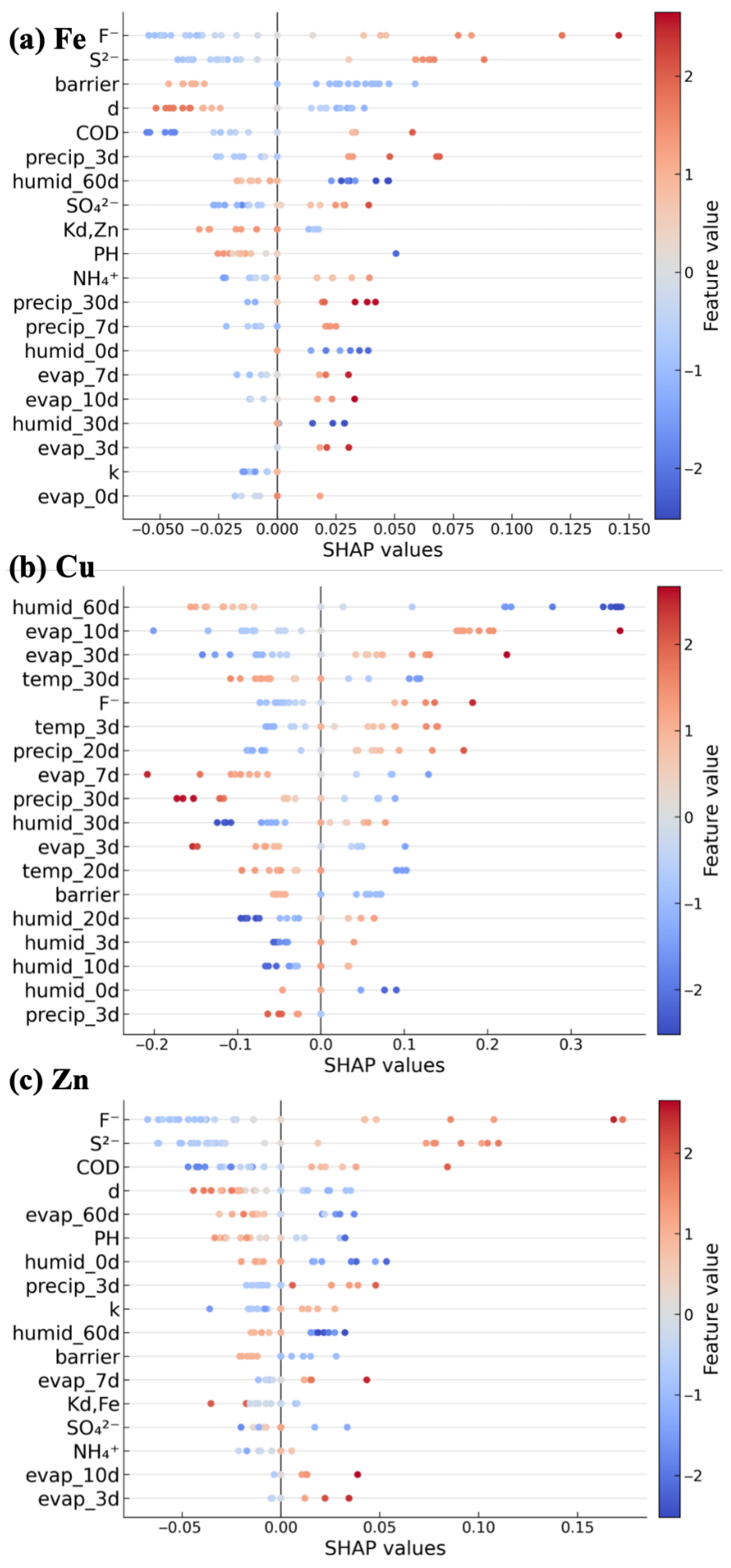
CH parameters contributed the second most to Fe cation concentration predictions, with an overall ACW of 32.7% (Figure 4a), wherein cumulative precipitation (from 3 to 60 days) and evaporation were two most important contributors, with ACWs of 7.0% and 8.7%, respectively (Figure 4a). These results suggest that precipitation-leached iron cations from waste rock piles and the reservoir, as well as recent local evaporation, are major processes that influence AMD prevalence. The analytical solution to a one-dimensional solute transport equilibrium yielded a time of 8 days for an iron cation (Fe3+ or Fe2+) to travel from the barrier (where possible reservoir leakage occurred before barrier installation) to the farthest monitoring well (W06). This estimate falls within the time frame of key cumulative precipitation times that were evaluated (3, 60, and 30 days; in the order of importance). However, numerical simulations indicated that infiltration from surface rainfall or snowfall (up to 109.2 mm/day during the monitoring period) to the groundwater table takes at least 3 days, during which Fe3+ dilution occurs. Cumulative precipitation over 10, 30, and 60 days was negatively correlated with iron concentrations (Figure 5a), suggesting that dilution is a major process that influences Fe cation concentrations. Cumulative evaporation over 60 days was the most influential single climate factor (ACW of 2.9%), suggesting that evaporation-induced water loss in soils eventually concentrates iron cations. Nevertheless, cumulative evaporation over 60 days was negatively correlated with iron concentrations (Figure 5a). Detailed analysis of the time history of cumulative evaporation and Fe concentrations from observation wells (Figure S5) revealed that peak evaporation timing was often in October and precedes peak iron concentration timing by 0–2 months. Concomitantly, cumulative evaporation minima usually occurred from February to April and preceded local Fe concentration minima by 0–2 months. The delay in Fe concentration changes is likely due to water rebalancing and solute redistribution in both the vadose and saturated zones. Cumulative evaporation created Fe concentration cycles with peaks and lows that mirrored evaporation patterns but lagged by up to two months, i.e., roughly one quarter of the annual evaporation cycle. Consequently, the annual cycle of iron concentration dynamics is approximately two-thirds (i.e., 120 degrees) out of phase with the annual evaporation cycle, leading to the observed negative contribution. Humidity and temperature were the two other important CH parameters and were highly correlated with precipitation and evaporation (Figure S8), following the same trends discussed above. Their individual contributions are consequently not further elaborated upon.
Geological parameters were the third most important contributors to iron concentration, with importance following the order of distance (d), Kd,Fe, permeability (k), and barrier installation. In other words, iron cation concentrations from the upstream reservoir conformed to the solute transport formula (Appendix A), whereas the contributions to mass transportation followed the order of diffusion (d), adsorption (Kd,Fe), and advection (k). The assumed order of diffusion > adsorption > advection is not always applicable in real solute transport processes. The relatively low feature importance of Kd,Fe and permeability may result from their limited variation (Table 1), thereby limiting their contributions to overall predictions. In addition, the construction of the low-permeability barrier significantly reduced the spread of heavy metal cations (Figure S5 and Figure 4a).

3.5. Parametric Analysis of Cu Concentration Predictions

Climate history parameters were as the most important contributors to Cu prediction, with an ACW of 86.9% (Figure 4b). The contributions of cumulative evaporation to the predicted Cu concentration were most important in the order of 10, 7, 30, and 3 days (Figure 4b). Specifically, cumulative evaporation over 10 and 30 days was positively correlated with Cu concentration (Figure 5b), suggesting that evaporation plays an important role in concentrating Cu2+ in subsurface waters over a timeframe suitable for water rebalance and Cu2+ redistribution (discussed above in Section 3.3). Decreasing Cu2+ concentration with increasing distance, along with a notable reduction following the installation of the barrier, suggests that the primary source of Cu2+ is the upstream reservoir. The cumulative precipitation over the preceding 20 days (Precip_20d) was positively correlated with Cu concentration, with an observed ACW of 5.1% (Figure 5b). Conversely, dilution, as represented by the cumulative precipitation of the preceding 30 days (precip_30d) exhibited an ACW of 4.4%, consequently representing a secondary influence that was negatively correlated with Cu concentrations (Figure 5b). The lack of a consistent temporal trend in cumulative precipitation indicates that both upstream leakage and local dilution concurrently occurred. A closer look at Cu concentrations and precip_30d trends shows that high precip_30d values (usually in June and August) match Cu concentration lows. In contrast, low precip_30d values (e.g., June and December 2019; February and October 2021) align with Cu concentration peaks, including December 2020 (Figure S6). These temporal associations provide clear evidence of a negative relationship between rainfall (or snowfall) and Cu2+ concentrations, thereby supporting the dilution hypothesis.
F and Cu2+ form CuF2, whose high solubility (46.71 g/L) [47] dictates the co--release or fixation of both F and Cu2+. Consequently, F and Cu2+ concentrations were highly correlated (ACW of 59.1% for the AWQ parameters; Figure 4b), which may also be due to their shared source and transport pathway. In contrast, the solubility of CuS is extremely low (8.55 × 10⁻¹⁷ g/L) [48]. Consequently, S2− concentrations are not necessarily related to Cu2+ (Figure S4b). The association between S2− and Cu2+ concentrations (ACW of 18.4% in AWQ, Figure 4b) is however attributed to shared sources and transport pathways.
After barrier installation, average Cu concentration values from six wells decreased from 0.96 mg/L to 0.25 mg/L, representing a 73.96% reduction. The reduction contributes to the 73.8% ACW that can be attributed to geological parameters (i.e., 3.5% out of the total 4.7% contribution of geological factors; Figure 4b). Considering the geological parameters, permeability, distance, and Kd,Cu contributed 12.1%, 9.7%, and 4.3%, respectively—values consistent with the 73.8% relative importance attributed to geological parameters altogether.

3.6. Parametric Analysis of Zn Concentration Predictions

The primary contributors to predicted Zn concentrations were AWQ parameters (ACW of 45.0%), followed by CH (ACW of 35.7%) and GEO (ACW of 19.3%) parameters (Figure 4c). Zn2+ and F originate from ZnF2 that exhibits high solubility in water (16.33 g/L at 25 °C [49] The solubility promotes simultaneous release or fixation of both ions, resulting in a strong positive connection between Zn2+ and F (ACW of 18.8%, Figure 5c). In contrast, S2− and Zn2+ are not directly related via dissolution of ZnS, due to a low solubility of 3.1 × 10⁻¹¹ g/L [50] Yet, Zn2+ and S2− concentrations were still positively correlated (Figure 5c), exhibiting an ACW of 11.8%, that is again attributed to their shared origin and transport pathways.
Decreased Zn2+ concentrations with increasing distance from the reservoir, along with a marked reduction in concentrations following barrier installation (Figure S7), suggests that the upstream reservoir is the principal source of Zn2+. Further supporting this assertion, the cumulative precipitation over 3 days was positively correlated with Zn concentrations, exhibiting an ACW of 4.8% (Figure 5c). In addition, cumulative evaporation over 3, 7, and 10 days was positively correlated with Zn concentrations, with a total ACW of 3.1% (Figure 5c). This suggests that evaporation concentrates Zn2+ in subsurface waters via water loss, thereby facilitating solute redistribution over these time windows.
After barrier installation, average Zn concentrations across the six wells decreased from 0.728 to 0.155 mg/L, representing a 78.7% decrease. This reduction corresponds to a 38.8% ACW that could be attributed to geological parameters (i.e., 7.5% out of the total 19.3% GEO contribution; Figure 4c), followed by distance (37.1%), Kd,Zn (17.5%), and permeability (6.6%).

4. Conclusions

To enable more robust AMD predictions for a mine waste rock site, a comprehensive experimental analysis was conducted in this study over 3.5 years, with generation of 132 spatiotemporal datasets to enable AMD predictions. The datasets comprised concentrations for nine chemical species, including F, S2−, pH, SO 4 2 , NH 4 + , and COD, alongside compilation of geological and historical climate datasets. Three ML algorithms (SVM, RF, and XGBoost models) were then used to predict the concentrations of metal contaminants (Fe, Cu, Zn) using three sets of input variables, GEO, CH, AWQ (in order of accessibility). The following key results were observed:
(1)
Groundwater monitoring before and after the barrier installation revealed a significant reduction in Fe, Zn, and Cu concentrations, demonstrating the barrier’s effectiveness in limiting heavy metal transport. However, the high CV (>50%) and increased skewness of the heavy metal concentration, concentrations indicated substantial spatial-temporal variability and potential extreme values. These fluctuations are largely influenced by the regional hydrological cycle, especially during the wet season, which enhances leaching and pollutant mobility.
(2)
The combined use of all three input parameter sets (GEO, CH and AWQ) generally yielded the best predictions. The XGBoost predictions exhibited the highest R2 values for Fe (0.805) and Cu (0.773) concentrations, while SVM predictions provided the best predictive performance for Zn concentrations (R2 of 0.94). The use of two sets of input parameters (GEO and CH) generally yielded better prediction than the use of geological parameters alone. Given the general availability and affordability of climate history data, as well as the physical relationships between climate history and downstream contaminant concentrations, the combined use of these two sets of input parameters are recommended.
(3)
Associated water quality parameters, and especially F and S2− concentrations, are the most relevant for predicting both Fe and Zn concentrations, also ranking second most important for Cu concentration predictions. The shared upstream reservoir origin and downstream transportation pathways are the likely reasons these AWQs are good predictors for Fe and Zn concentrations, wherein the high solubility of FeF3 promotes the release or fixation of both Fe3+ and F, emphasizing their physical linkage.
(4)
Climate history was the most important factor for Cu concentration prediction and the second most important factor for Fe and Zn concentration predictions. Accumulated precipitation and evaporation up to 60 days are related to metal concentrations via dynamic water rebalance and solute redistribution mechanisms.
(5)
Installation of a vertical contaminant-containing barrier was the most effective geological parameter, followed by distance and the partition coefficient. All three metal contaminant concentrations were drastically reduced (73–80%) following barrier installation.
(6)
This study’s scope is confined to observations from a singular AMD reservoir site, potentially restricting the generalizability of the results to other settings. Enhancing the analysis by incorporating data from multiple copper mine AMD reservoir sites could bolster the reliability and wider relevance of the conclusions. Additionally, the utilization of remote sensing data offers valuable prospects for capturing spatial and temporal fluctuations in environmental factors. Subsequent research endeavors could investigate the integration of such data into the modeling framework to potentially elevate predictive precision and utility [22].
The results of this study provide a comprehensive evaluation of the factors governing AMD contamination monitoring and prediction. In particular, these results underscore the critical, but often underestimated role of climate history in shaping contaminant dynamics. This highlights the need to integrate climate history data into predictive frameworks, thereby promoting more robust, cost-effective, and physically informed strategies for environmental risk assessment and sustainable mine waste management.

Supplementary Materials

The following supporting information can be downloaded at: https://www.mdpi.com/article/10.3390/w17182661/s1, Text S1: Calculation of the distribution coefficient; Text S2: SHAP analysis; Table S1: Optimal Model Hyperparameters and Hyperparameter Optimization Results; Figure S1: Predicted versus measured concentrations for Fe (a, b, c) with prediction models exhibiting the highest R2 values. Red points indicate training datasets, green points indicate test datasets, the black line is the 1:1 prediction line, light green shading shows the 95% prediction confidence interval, and dark green shading shows the 95% prediction confidence interval; Figure S2: Predicted versus measured concentrations for Zn (a, b, c) with prediction models exhibiting the highest R2 values; Figure S3: Predicted versus measured concentrations for Cu (a, b, c) with prediction models exhibiting the highest R2 values; Figure S4: SHAP single analysis between (a) F and Fe, Cu, Zn; (b) S2− and Fe, Cu, Zn; and (c) distance and Fe, Cu, Zn; Figure S5: Temporal trends in Fe concentrations and cumulative evaporation over 60-day windows; Figure S6: Temporal trends in Cu concentrations and cumulative precipitation over 30-day windows; Figure S7: Temporal trends in Zn concentrations and cumulative precipitation over 30-day windows; Figure S8: Pearson correlation coefficients for 37 parameters within the GEO, CH, AWQ datasets and the 3 target metal concentrations (*: p value < 0.05).

Author Contributions

Conceptualization, B.W. and B.B.; data curation, A.D. and Q.W.; formal analysis, X.W., B.W. and B.B.; funding acquisition, B.B.; investigation, A.D. and Q.W.; methodology, Y.L. and Z.C.; project administration, X.W.; resources, X.W. and A.D.; software, B.W.; supervision, B.W. and B.B.; validation, X.W. and B.B.; visualization, X.W. and B.W.; writing—original draft, B.W. and X.W.; writing—review and editing, B.W. and X.W. All authors have read and agreed to the published version of the manuscript.

Funding

This work is funded by the National Natural Science Foundation of China (Award No.: 42177118), the Ministry of Science and Technology of China (Award No.: 2019YFC1805002) and the Basic Science Center Program for Multiphase Evolution in Hypergravity of the National Natural Science Foundation of China (Award No.: 51988101).

Data Availability Statement

The original contributions presented in this study are included in the article/Supplementary Material. Further inquiries can be directed to the corresponding author(s).

Acknowledgments

We thank LetPub for its linguistic assistance during the preparation of this manuscript. Available online: https://www.letpub.com.cn (accessed on 3 July 2025).

Conflicts of Interest

Authors Xinyu Wu, Aifang Du and Qiong Wang were employed by the company Beijing General Research Institute of Mining and Metallurgy Technology Group Co., Ltd. The remaining authors declare that the research was conducted in the absence of any commercial or financial relationships that could be construed as a potential conflict of interest.

Abbreviations

ACW, accumulated contribution weights; AMD, Acid mine drainage; AWQ, associated water quality; CH, climate history; evap, Evaporation; GEO, geolog-ical; MAE, Mean Absolute Error; MSE, Mean Squared Error; ML, machine learning; precip_nd, the cumulative precipitation over the preceding n days; R2, the Coefficient of Determination (R2); RMSE, Root Mean Squared Error; SVM, support vector machine; WI, Willmott Index; XGBoost, extreme gradient boosting.

Appendix A

c ( x , t ) = M 4 π D e ( t i t 1 ) exp ( x u e ( t i t 1 ) ) 2 4 D e ( t i t 1 )
R = 1 + ρ b θ K d
where c ( x , t ) is the solute concentration at position x and time t. M is the total mass released per unit cross-sectional area, D e is the effective dispersion coefficient, u e is the effective solute velocity, t i and t l are specific times, and R is the retardation factor.

References

  1. Lefebvre, R.; Hockley, D.; Smolensky, J.; Gélinas, P. Multiphase transfer processes in waste rock piles producing acid mine drainage: 1: Conceptual model and system characterization. J. Contam. Hydrol. 2001, 52, 137–164. [Google Scholar] [CrossRef]
  2. Gao, T.; Wu, A.; Wang, S.; Ruan, Z.; Chen, C.; Sun, W. Compression behavior and microscopic damage mechanism of waste rock-tailings matrix composites: Experiments and models. Constr. Build. Mater. 2024, 425, 136076. [Google Scholar] [CrossRef]
  3. Cánovas, C.; Olías, M.; Macias, F.; Torres, E.; San Miguel, E.; Galván, L.; Ayora, C.; Nieto, J. Water acidification trends in a reservoir of the Iberian Pyrite Belt (SW Spain). Sci. Total Environ. 2016, 541, 400–411. [Google Scholar] [CrossRef] [PubMed]
  4. Zhou, S.; Yang, Y.-X.; Cao, J.-J.; Meng, L.-L.; Cao, J.-N.; Zhang, C.; Zhang, S.; Bate, B. Monitoring of copper adsorption on biochar using spectral induced polarization method. Environ. Res. 2024, 251, 118778. [Google Scholar] [CrossRef] [PubMed]
  5. Kalin, M.; Fyson, A.; Wheeler, W.N. The chemistry of conventional and alternative treatment systems for the neutralization of acid mine drainage. Sci. Total Environ. 2006, 366, 395–408. [Google Scholar] [CrossRef] [PubMed]
  6. Chen, G.; Ye, Y.; Yao, N.; Hu, N.; Zhang, J.; Huang, Y. A critical review of prevention, treatment, reuse, and resource recovery from acid mine drainage. J. Clean. Prod. 2021, 329, 129666. [Google Scholar] [CrossRef]
  7. Dong, Y.; Liu, Z.; Lin, H. Hydrophobic modification of pyrite with a composite of sodium oleate and SiO2 nanoparticles to inhibit its oxidation for controlling acid mine drainage. J. Environ. Chem. Eng. 2023, 11, 109571. [Google Scholar] [CrossRef]
  8. Lin, H.; Zhi, T.; Zhang, L.; Liu, C.; Dong, Y. Effects of acid/alkali-pretreated peanut shells as a cheap carbon source for the bio-reduction of sulfate. J. Clean. Prod. 2023, 385, 135753. [Google Scholar] [CrossRef]
  9. Yuan, S.; Han, G.; Liang, Y. Groundwater control in open-pit mine with grout curtain using modified lake mud: A case study in East China. Arab. J. Geosci. 2021, 14, 1148. [Google Scholar] [CrossRef]
  10. Cacciuttolo, C.; Pastor, A.; Valderrama, P.; Atencio, E. Process water management and seepage control in tailings storage facilities: Engineered environmental solutions applied in Chile and Peru. Water 2023, 15, 196. [Google Scholar] [CrossRef]
  11. Wu, Q.; Li, X.; Feng, Q.; Li, X. Source reduction and end treatment of acid mine drainage in closed coal mines of the Yudong River Basin. Water Sci. Technol. 2024, 89, 470–483. [Google Scholar] [CrossRef] [PubMed]
  12. Yuan, S.; Sun, B.; Han, G.; Duan, W.; Wang, Z. Application and prospect of curtain grouting technology in mine water safety management in China: A review. Water 2022, 14, 4093. [Google Scholar] [CrossRef]
  13. Shi, Y.; Li, Z.; Liang, M.; Hu, H.; Chen, S.; Duan, L.; Chen, Z.; Yang, X.; Cai, J. Experimental study on the stabilization and anti-seepage treatment of lead and zinc elements in heavy metal tailings pond using cement slurry containing heavy metal stabilizing agent. Constr. Build. Mater. 2024, 425, 135964. [Google Scholar] [CrossRef]
  14. Li, X.; Ren, H.; Xu, Z.; Chen, G.; Zhang, S.; Zhang, L.; Sun, Y. Practical application for legacy acid mine drainage (AMD) prevention and treatment technologies in karst-dominated regions: A case study. J. Contam. Hydrol. 2023, 258, 104238. [Google Scholar] [CrossRef] [PubMed]
  15. Cacciuttolo, C.; Cano, D. Environmental impact assessment of mine tailings spill considering metallurgical processes of gold and copper mining: Case studies in the Andean countries of Chile and Peru. Water 2022, 14, 3057. [Google Scholar] [CrossRef]
  16. Rooki, R.; Doulati Ardejani, F.; Aryafar, A.; Bani Asadi, A. Prediction of heavy metals in acid mine drainage using artificial neural network from the Shur River of the Sarcheshmeh porphyry copper mine, Southeast Iran. Environ. Earth Sci. 2011, 64, 1303–1316. [Google Scholar] [CrossRef]
  17. Kabuba, J.; Maliehe, A.V. Application of neural network techniques to predict the heavy metals in acid mine drainage from South African mines. Water Sci. Technol. 2021, 84, 3489–3507. [Google Scholar] [CrossRef]
  18. Trifi, M.; Gasmi, A.; Carbone, C.; Majzlan, J.; Nasri, N.; Dermech, M.; Charef, A.; Elfil, H. Machine learning-based prediction of toxic metals concentration in an acid mine drainage environment, northern Tunisia. Environ. Sci. Pollut. Res. 2022, 29, 87490–87508. [Google Scholar] [CrossRef]
  19. Li, Y.; Liu, Y.; Fu, Y.; Liu, Z.; Wang, P.; Yin, J.; Kou, J.; Sun, C.; Liu, W. Enhanced leaching of copper from refractory oxidized copper ore by calcium fluoride: Behavior and mechanism. Green Smart Min. Eng. 2024, 1, 85–95. [Google Scholar] [CrossRef]
  20. Hasrod, T.; Nuapia, Y.B.; Tutu, H. Comparison of individual and ensemble machine learning models for prediction of sulphate levels in untreated and treated Acid Mine Drainage. Environ. Monit. Assess. 2024, 196, 332. [Google Scholar] [CrossRef]
  21. Zhao, S.; Chen, K.; Xiong, B.; Guo, C.; Dang, Z. Prediction of adsorption of metal cations by clay minerals using machine learning. Sci. Total Environ. 2024, 924, 171733. [Google Scholar] [CrossRef]
  22. Nordstrom, D.K. Acid rock drainage and climate change. J. Geochem. Explor. 2009, 100, 97–104. [Google Scholar] [CrossRef]
  23. Anawar, H.M. Impact of climate change on acid mine drainage generation and contaminant transport in water ecosystems of semi-arid and arid mining areas. Phys. Chem. Earth Parts A/B/C 2013, 58, 13–21. [Google Scholar] [CrossRef]
  24. Liu, W.; Zhao, Y.; Chen, J.; Azam, M.; Asubonteng, D.; Ngoie, M.; Lin, S.; Sun, W. Advancements in Removing Fluorine from Copper Concentrate. Min. Metall. Explor. 2023, 40, 1487–1497. [Google Scholar] [CrossRef]
  25. Solid Waste—Determination of Metals—Inductively Coupled Plasma Mass Spectrometry (ICP-MS). Ministry of Ecology and Environment of the People’s Republic of China (MEE). 2015. Available online: https://std.samr.gov.cn/search/std?tid=&q=HJ766-2015 (accessed on 10 May 2025).
  26. Li, K.; Guo, G.; Zhang, D.; Lei, M.; Wang, Y. Accurate prediction of spatial distribution of soil potentially toxic elements using machine learning and associated key influencing factors identification: A case study in mining and smelting area in southwestern China. J. Hazard. Mater. 2024, 478, 135454. [Google Scholar] [CrossRef] [PubMed]
  27. Li, H.; Pang, Y.; Ding, Y.; Fan, Z.; Xu, Y.; Liu, W. Data-driven machine learning modeling reveals the impact of micro/nanoplastics on microalgae and their key underlying mechanisms. J. Hazard. Mater. 2025, 496, 139338. [Google Scholar] [CrossRef]
  28. Breiman, L. Random forests. Mach. Learn. 2001, 45, 5–32. [Google Scholar] [CrossRef]
  29. Belgiu, M.; Drăguţ, L. Random forest in remote sensing: A review of applications and future directions. ISPRS J. Photogramm. Remote Sens. 2016, 114, 24–31. [Google Scholar] [CrossRef]
  30. Parmar, A.; Katariya, R.; Patel, V. A review on random forest: An ensemble classifier. In Proceedings of the International Conference on Intelligent Data Communication Technologies and Internet of Things, Coimbatore, India, 7–8 August 2018; pp. 758–763. [Google Scholar]
  31. Chen, T.; Guestrin, C. Xgboost: A scalable tree boosting system. In Proceedings of the 22nd ACM SIGKDD International Conference on Knowledge Discovery and Data Mining, San Francisco, CA, USA, 13–17 August 2016; pp. 785–794. [Google Scholar]
  32. Chen, T.; He, T.; Benesty, M.; Khotilovich, V.; Tang, Y.; Cho, H.; Chen, K.; Mitchell, R.; Cano, I.; Zhou, T. Xgboost: Extreme Gradient Boosting, R Package Version 0.4-2; Scientific Research Publishing Inc.: Wuhan, China, 2015. [CrossRef]
  33. Jakkula, V. Tutorial on support vector machine (svm). Sch. EECS Wash. State Univ. 2006, 37, 3. [Google Scholar] [CrossRef]
  34. Joachims, T. Making Large-Scale SVM Learning Practical; Technical Report No. 1998,28; Universität Dortmund: Dortmund, Germany, 1998. [Google Scholar]
  35. Standard for Groundwater Quality. Standardization Administration of China (SAC). 2017. Available online: https://std.samr.gov.cn/search/std?q=GB/T14848-2017 (accessed on 10 May 2025).
  36. Barroso, A.; Henriques, R.; Cerqueira, Â.; Gomes, P.; Antunes, I.M.H.R.; Reis, A.P.M.; Valente, T.M. Acid mine drainage and waste dispersion in legacy mining sites: An integrated approach using UAV photogrammetry and geospatial analysis. J. Hazard. Mater. 2025, 495, 138827. [Google Scholar] [CrossRef]
  37. Domingos, P. A few useful things to know about machine learning. Commun. ACM 2012, 55, 78–87. [Google Scholar] [CrossRef]
  38. Xu, Z.; Wang, Z. A risk prediction model for type 2 diabetes based on weighted feature selection of random forest and xgboost ensemble classifier. In Proceedings of the 2019 Eleventh International Conference on Advanced Computational Intelligence (ICACI), Guilin, China, 7–9 June 2019; pp. 278–283. [Google Scholar]
  39. Dhaliwal, S.S.; Nahid, A.-A.; Abbas, R. Effective intrusion detection system using XGBoost. Information 2018, 9, 149. [Google Scholar] [CrossRef]
  40. Liu, W.; Chen, Z.; Hu, Y. XGBoost algorithm-based prediction of safety assessment for pipelines. Int. J. Press. Vessel. Pip. 2022, 197, 104655. [Google Scholar] [CrossRef]
  41. Cevikalp, H. Best fitting hyperplanes for classification. IEEE Trans. Pattern Anal. Mach. Intell. 2016, 39, 1076–1088. [Google Scholar] [CrossRef] [PubMed]
  42. Hao, R.; Yin, W.; Jia, H.; Xu, J.; Li, N.; Chen, Q.; Zhong, Z.; Wang, J.; Shi, Z. Dynamics of dissolved heavy metals in reservoir bays under different hydrological regulation. J. Hydrol. 2021, 595, 126042. [Google Scholar] [CrossRef]
  43. Hutter, F.; Kotthoff, L.; Vanschoren, J. Automated Machine Learning: Methods, Systems, Challenges; Springer Nature: Berlin/Heidelberg, Germany, 2019. [Google Scholar]
  44. Gholami, R.; Kamkar-Rouhani, A.; Doulati Ardejani, F.; Maleki, S. Prediction of toxic metals concentration using artificial intelligence techniques. Appl. Water Sci. 2011, 1, 125–134. [Google Scholar] [CrossRef]
  45. Maulana, A.; Irfan, U.R. Characteristic of Alteration and Mineralization of Sulfide Deposits at Sasak area, Tana Toraja, Indonesia. In Proceedings of the IOP Conference Series: Earth and Environmental Science, Surabaya, Indonesia, 25–26 October 2023; p. 012029. [Google Scholar] [CrossRef]
  46. Gálvez, J.L.; Dufour, J.; Negro, C.; López-Mateos, F. Determination of iron and chromium fluorides solubility for the treatment of wastes from stainless steel mills. Chem. Eng. J. 2008, 136, 116–125. [Google Scholar] [CrossRef]
  47. Gallagher, T.C.; Sandstrom, S.K.; Wu, C.-Y.; Stickle, W.; Fulkerson, C.R.; Hagglund, L.; Ji, X. Copper metal electrode reversibly hosts fluoride in a 16 m KF aqueous electrolyte. Chem. Commun. 2022, 58, 10218–10220. [Google Scholar] [CrossRef]
  48. Su, H.; Qian, X.; Gu, Z.; Xu, Z.; Lou, H.; Bian, X.; Zeng, T.; Lin, D.; Filser, J.; Li, L. Cu(OH)2 nanorods undergo sulfidation in water: In situ formation of CuO nanorods as intermediates and enhanced toxicity to Escherichia coli. Environ. Chem. Lett. 2020, 18, 1737–1744. [Google Scholar] [CrossRef]
  49. Li, H.; Wang, S.; Zeng, D. Experimental measurement of the solid–liquid equilibrium of the systems MF2 + H2O (M = Mg, Ca, Zn) from 298.15 to 353.15 K. J. Chem. Eng. Data. 2018, 63, 1733–1736. [Google Scholar] [CrossRef]
  50. Yang, K.; Li, B.; Zeng, G. Effects of temperature on properties of ZnS thin films deposited by pulsed laser deposition. Superlattices Microstruct. 2019, 130, 409–415. [Google Scholar] [CrossRef]
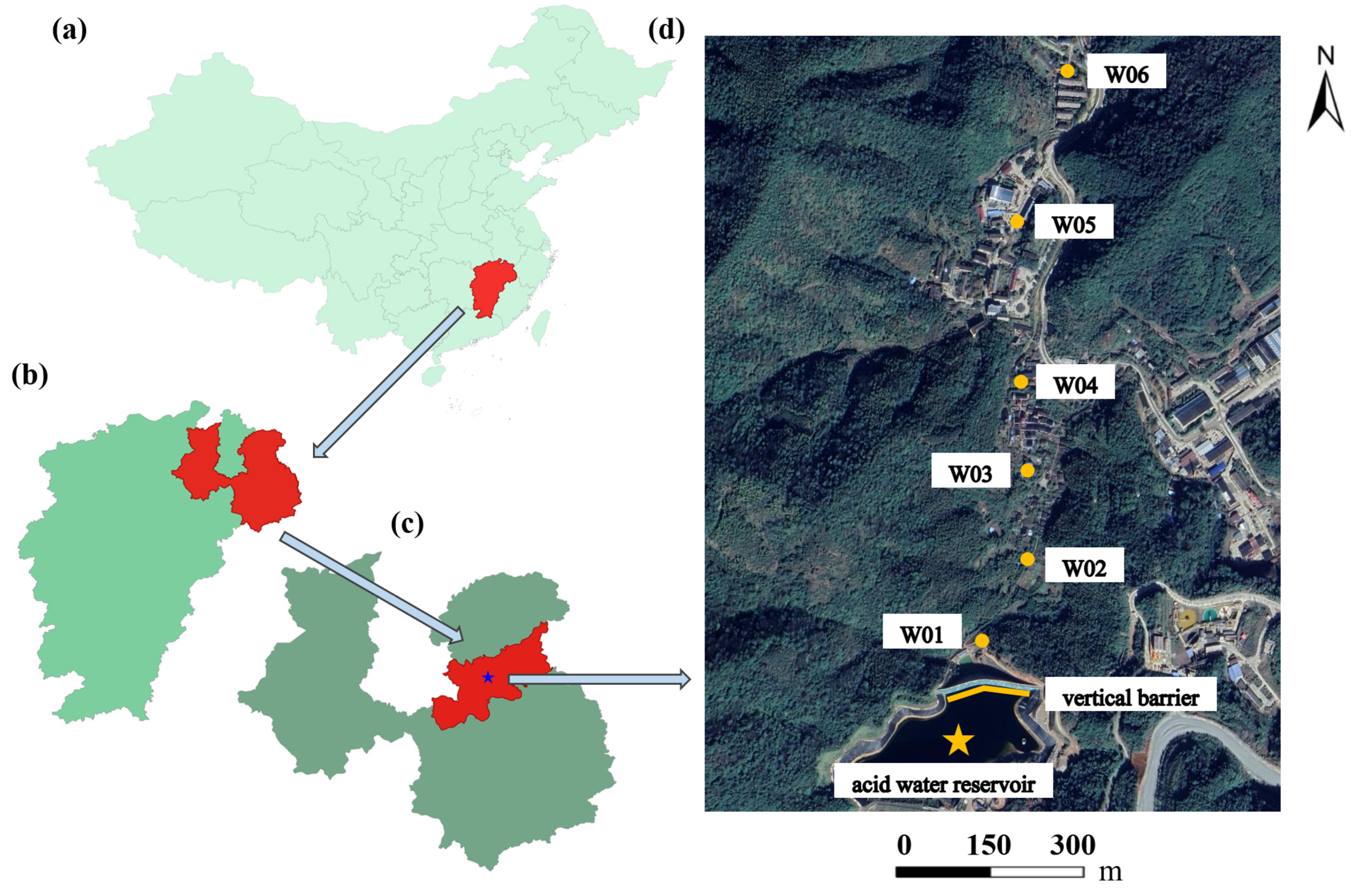
Figure 1. Groundwater sampling sites in the study area. (a) Jiangxi Province in China. (b) Shangrao City within Jiangxi Province. (c) Dexing City within Shangrao. (d) Monitoring wells downstream of the reservoir at the mine waste rock site.
Water 17 02661 g001
Figure 2. Workflow chart for predicting heavy metal concentrations.
Water 17 02661 g002
Figure 3. Heavy metal concentrations before and after barrier installation, along with statistical parameters; n: number of samples; Mean: average value of heavy metal concentration; Std: standard deviation; Skew: skewness; CV: coefficient of variation; Risk value: Class III groundwater quality thresholds (MNR, 2017).
Water 17 02661 g003
Figure 4. Feature importance rankings for the predictive models that included climate history datasets over 0, 3, 7, 10, 20, 30, and 60 days prior to sampling. “GEO” indicates geological parameters, “CH” indicates climate history-related parameters, and “AWQ” indicates associated water quality parameters.
Water 17 02661 g004
Figure 5. Summary of SHAP analysis for Fe, Cu, and Zn concentrations.
Water 17 02661 g005
Table 1. GEO parameter information for the investigated mine waste rock site.
Well IDd (m)Kd,CuKd,FeKd,Znk
W0129948.412.77.70.091
W0243294.1340.9134.50.091
W0357577.6627.215.80.091
W0485564.72914.73.00.085
W05121953.9740.564.30.081
W06156257.6691.9126.50.084
Disclaimer/Publisher’s Note: The statements, opinions and data contained in all publications are solely those of the individual author(s) and contributor(s) and not of MDPI and/or the editor(s). MDPI and/or the editor(s) disclaim responsibility for any injury to people or property resulting from any ideas, methods, instructions or products referred to in the content.