Abstract
The topography of the flood path significantly influences the hydraulic characteristics of flood events, necessitating in-depth analysis to better understand the continuous dynamics during dam failure scenarios. These analyses are useful for the hydraulic evaluation of infrastructures downstream of a dam site. This study examined the effects of four distinct converging configurations of guide-banks on the propagation of unsteady flow in a rectangular channel. The configurations studied included trapezoidal and crescent side contractions, as well as trapezoidal and crescent barriers located at the channel’s center, each with varying lengths and widths. Numerical simulations using computational fluid dynamics (CFD) simulation were validated against experimental data from the literature. The results reveal that the flow experienced a depth increase upon encountering converging geometries, leading to the formation of a hydraulic jump and the subsequent upstream progression of the resulting wave. The width of the obstacles and contractions had a marked influence on the flow profile. Increased channel contraction led to a more pronounced initial water elevation rise when the flood flow encountered the topography, resulting in a deeper reflected wave that propagated upstream at less time. The reflected wave increased the water elevations up to 0.64, 0.72, and 0.80 times the initial reservoir level (0.25 m), respectively, for cases with 33%, 50%, and 66% contraction ratios to the channel width (0.3 m). For the same cases at a certain time of t = 5.0 s, the reflected wave reached 1.1 m downstream, 0.5 m downstream, and 0.1 m upstream of the initial dam location. Waves generated by the trapezoidal configuration affected the upstream in less time than those formed by the crescent contraction. The length of the transitions or their placement (middle of/across the channel) did not significantly affect the flow profile upstream; however, within the converging zone, longer configurations resulted in a wider increased water elevation. Overall, the intensity of the hydraulic response can be related to one factor in all cases, namely, the convergence intensity of the flow lines as they entered the contractions.
1. Introduction
Floods are among the most catastrophic hydrological events, capable of causing severe damage to infrastructure and significant loss of life [1,2]. While in many cases single structures, such as dams, or hybrid structures that combine various flood control measures, are typically among the best options to manage floods [3,4], their failure can also serve as a significant source of flooding in downstream areas. Among the various types of floods, dam-break floods stand out as particularly devastating due to their rapid onset, immense destructive potential, and widespread impact on both infrastructure and human populations [5]. It is expected that the frequency and intensity of extreme weather events be exacerbated, potentially increasing the likelihood of conditions that could lead to dam failures and subsequent floods [6,7]. Hence, understanding the hydraulic response of dam-break waves to different channel geometries is crucial for improving flood risk assessments and designing effective mitigation strategies.
Several factors influence the characteristics and impact of dam-break floods, including the reservoir volume [8], breach formation dynamics [9], downstream topography [10], and channel boundary conditions [11]. The breach development determines the release rate and peak discharge of the flood wave [12]. Hydrodynamic factors such as flow resistance, bed roughness, and sediment transport further modulate wave attenuation and energy dissipation [13,14]. Additionally, external influences such as vegetation [15], infrastructure [16], and tributary inflows [17] can alter flood propagation patterns. Among these factors, channel morphology plays a particularly critical role in shaping the evolution of dam-break waves. Variations in channel slope [18], width [19], sinuosity [20], and cross-sectional geometry [10] influence wave speed, depth, and flood extent. Constrictions or expansions in the channel can also cause wave reflection, energy concentration, or dispersion, significantly altering the flood’s destructive potential [21,22]. Understanding these morphological controls is essential for accurate flood hazard predictions and the development of effective mitigation strategies. To comprehensively assess the implications of such an event and to provide a reliable estimate of the associated flood risk, it is essential to investigate various dam failure scenarios. These scenarios can generally be categorized into two groups. The first category involves case studies and numerical simulations aimed at fully modeling the routing of the dam breach flow and examining their propagation through rivers, canals, and urban infrastructure downstream [23,24,25,26,27,28]. The second category does not relate to complete routing of a dam-break flood but encompasses studies that investigate the dam-break flow dynamics in a closed domain, typically conducted at a laboratory scale, and identify the influence of various factors on the flood. The present study falls into the second category and primarily examines the interaction between floods and structures during a dam-break event.
The water–structure interaction is particularly significant downstream of a failed dam [23]. Unlike river floods, dam-break floods occur much more abruptly and with higher flow velocities, making their impact on downstream. In the event triggered by a dam failure, the flow typically traverses a heterogeneous topography at downstream, influencing its hydraulic characteristics. Various factors such as the presence of bridge piers in the river path, flow-facing structures, changes in channel width, steps or protrusions in the channel invert, and vegetation can significantly alter the flood’s flow profiles. Additionally, infrastructures such as roads, bridges, and municipal facilities serves as barriers to the downstream propagation of flood waves following a dam failure [29]. These variations lead to the formation of secondary waves and increasing water turbulence, thereby heightening the potential for more extensive damage. Kocaman et al. [19] investigated the impact of three trapezoidal transitions with varying geometries onto a dam-breach flow in a rectangular channel. Their research focused on flow profiles during the sudden emptying process of a reservoir due to the abrupt removal of a gate. The study found that the flow depth increased as it passed through the transitions, and this increase propagated upstream as a form of a wave. Additionally, they numerically modeled their experiments and demonstrated that the set of Reynolds-Averaged Navier–Stokes (RANS) equations using the standard k-ε turbulence model successfully reproduce the flow profile of a dam-break unsteady flow in similar geometries. Kocaman et al. [30] experimentally and numerically explored the propagation of flood waves resulting from a dam breach in a region with closed boundaries. In their scenario, waves propagate not only downstream but also upstream, as the flow interacts with the boundaries. Their study specifically focused on the effect of tailwater depth on the resulting wave profile. The reliability of RANS equations with a standard k-ε turbulence model coupled with VOF method in simulating wave propagation is reported in their work. Di Cristo et al. [31] introduced two morphodynamic models to analyze the interaction between a dam-break wave and a rigid obstacle in the presence of an erodible bed. Their study emphasized the importance of developing effective predictive tools for assessing impact forces on structures caused by floods, which are crucial for designing appropriate risk mitigation strategies and protective measures. Khoshkonesh et al. [29] conducted a numerical study on two configurations of individual obstacles placed downstream of a dam-break wave. In their model, the obstacles were arranged in a triangular formation within a rectangular channel, allowing the flow to pass through them. Their findings highlighted the significant influence of obstacle arrangement on key hydraulic parameters, including the flow profile, reservoir discharge rate, three-dimensional velocity fields, and flow regimes around the obstacles. Maghsoodi et al. [32] investigated three different scenarios of obstacle arrangement facing a dam-break wave, namely, a rectangular obstacle, a trapezoidal sill, and triangle sill in a channel path. A set of RANS equations with a standard k-ω turbulence model along with a VOF tracking method were used in their study to analyze flow profiles and pressure field with sufficient accuracy. Lee and Nguyen [33] performed numerical simulations using an LES turbulence model coupled with a VOF tracking method to investigate the hydraulic characteristics of a dam-break flood in a laboratory-scale urban area. The variables of their problem included initial water stage, breach size, and position of dam gate. They analyzed flow depth contours, the velocity hydrograph, streamlines, vorticity, and the q-criterion incorporated with these variables. Focusing on wave–structure interactions, Oodi et al. [34] investigated the transient flow characteristics of dam-break waves interacting with downstream obstacles and contractions at varying distances in a channel site. They developed a high-accuracy numerical code by incorporating an LES turbulence model along with an air entrainment model and the VOF method to analyze flow profiles, turbulence structures, air entrainment around obstacles, flow regime variations, and the flood hydrograph in the downstream channel. Their findings contribute to a deeper understanding of the wave–structure interactions during dam-break events by elucidating how obstacles influence wave dynamics at different distances from the dam. Beteille et al. [35] experimentally and numerically studied the dam-break flood in an idealized city layout with reduced scale. They analyzed the impact of different configurations of cubic obstacles on the flow field characteristics including flow depth history and instantaneous velocity around the obstacles. The VOF-based RANS model in their study was able to accurately reproduce wake zones around the obstacles and the velocity field.
While numerous scenarios of wave–structure interactions during a dam-break include the presence of obstacles in an idealized urban area, the intention of the present work is to study the transient flood flow across a river site. The presence of hydraulic structures in a river site is common, and the failure of them can lead to rapid propagation of flood waves across a river and colliding with infrastructure located in or across the river, therefore making it practical to study. In present study, the interacting infrastructures were specifically defined based on practical river control structures. Among them, the presence of “guide-banks” in a river site were evaluated during a dam-break event, which has not been investigated with a focused manner in previous research. Guide-banks are built for guiding and regulating the river flow for various reasons. They can be used for preventing erosion and ensuring safe passage of water around bridges, weirs, and hydraulic structures. They can be constructed in pairs, upstream and downstream of the supported structure, and can be parallel, convergent, or divergent depending on the specific needs of the river and the structure [36,37]. In present work, four different guide-bank placements along a river path were evaluated facing a dam-break flood in a rectangular channel—this includes lateral and mid-width contractions with either trapezoidal or crescent shape. In addition, for each case, various configurations of length and contraction width for guide-banks were assessed. The evaluated configurations covered a reasonable range of guide-bank designs, representing practical results for engineering applications [37]. This study assessed key hydraulic parameters, including flow profiles and velocity fields of the dam-break wave, influenced by various downstream contractions. The findings contribute to a deeper understanding of flood dynamics in river systems following different configurations of guide-banks. The findings will be useful for flood risk management and also can be incorporated for designing and evaluating river guide-banks. Furthermore, this study aims to develop a high-accuracy numerical model capable of predicting flood characteristics resulting from dam failures in channels interacting with downstream constrictions.
2. Materials and Methods
2.1. Numerical Model Description
A Computational Fluid Dynamics (CFD) model was applied to simulate the three-dimensional flow dynamics of the problem. The reference model of this study was adapted from the experiment work of Kocaman et al. [19]. As illustrated in Figure 1, the setup consists of a rectangular channel with a width of 30 cm and a zero-bed slope. At t = 0 (t is time), a still water region with a height of 25 cm exists upstream of the gate’s location. The gate has not been modeled. The simulation begins with the sudden releasing of initial water, initiating an unsteady flow downstream while the water upstream gradually drained over time. Throughout this drainage process, no additional inflow is introduced into the computational domain. Downstream of the gate’s initial position (set as the origin coordinates system), two converging transitions with a trapezoidal shape in plan are present, significantly influencing the characteristics of the unsteady flow.
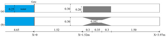
Figure 1.
Descriptions of the reference model [19]: (a) side view; (b) plan view.
In this study, following the simulation of the reference model based on the geometric specifications outlined in Figure 1 and the validation of the results using the experimental data of Kocaman et al. [19] (as detailed in Section 2.4), new geometries in the channel plan were assembled in the numerical model. The tested configurations fell into four categories as shown in Figure 2, namely, parallel lateral contraction with trapezoidal shape (Tr), parallel lateral contraction with crescent shape (Cr), parallel mid-width contraction with trapezoidal shape (Tr-C), and parallel mid-width contraction with crescent shape (Cr-C). In each category, the transition was considered with three contraction ratios along with three various lengths. The channel widths at the contraction (LC) were selected as 0.1, 0.15, and 0.2 m, which corresponded to contraction ratios of 0.66, 0.5, and 0.33 compared to the channel width (0.3 m). The overall lengths of transitions were selected as 0.6, 0.9, and 1.2 m in which the sloping sides of trapezoidal contractions were constant. These values corresponded to 2W, 3W, and 4W (W = channel width). Consequently, the tested cases provide a conclusion and cover a wide insight about the effect of the placement of guide-banks (lateral versus mid-width), shape of them (crescent versus trapezoidal), contraction ratios, and length of the transitions on the dam-break response in a channel. Overall, 36 distinct guide-bank geometries were evaluated in present study, all of which had a vertical height of 20 cm in numerical simulations. The descriptions of the numerical runs are represented as Table 1.
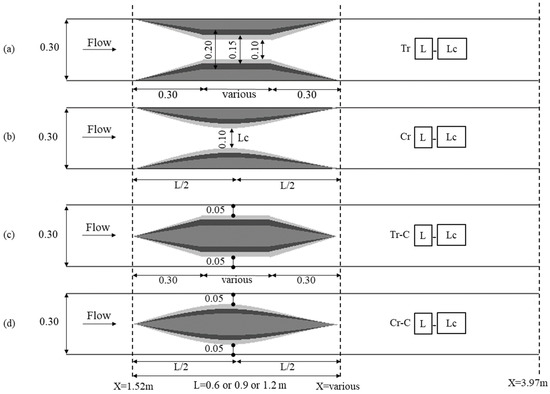
Figure 2.
Plan view of the channel contractions used in the numerical simulations of the present study (all dimensions are in meters): (a) parallel lateral contraction with trapezoidal shape, (b) parallel lateral contraction with crescent shape, (c) parallel mid-width contraction with trapezoidal shape, (d) parallel mid-width contraction with crescent shape.

Table 1.
Definition of numerical cases.
2.2. CFD Code
This CFD simulation demonstrates satisfactory performance in solving hydraulic problems involving both steady and unsteady flow in open channels, as validated in previous studies [19,30,38,39,40,41]. In this study, Reynolds-Averaged Navier–Stokes (RANS) equations were incorporated to solve the three-dimensional turbulent flow of an incompressible Newtonian fluid. In previous dam-break problems, the RANS approach provides a more accurate results compared to Shallow-Water Equations (SWE), especially in terms of the initial times of dam-break, and moreover provides better insights of the three-dimensional flow field around the obstacles [19,35,40,42,43]. On the other hand, the RANS approach is considered cost-effective in comparison with the Large Eddy Simulation (LES) method in terms of modeling turbulence. The conservation of mass and momentum equations are represented in three-orthogonal cartesian coordinates as Equations (1) and (2), respectively, in which they are discretized by the Finite Volume Method (FVM):
In these equations, x represents the coordinate along the three directions (denoted each time by the subscripts i and j), t is time, VF is the fractional volume open to flow, p is the pressure, ρ is the fluid density, ui is the mean velocity, Ai is the fractional area open to flow, gi is the body acceleration, and fi is the viscous acceleration in the subscript direction.
Three closure models, namely, the standard k-ε [44], the RNG k-ε [45], and the standard k-ω [46], were adopted to complete solving the RANS equations, and accuracies of them are compared in Section 2.4.2. All of these two-equation models have widespread use in dam-break problems in channels [19,32,35,40,41,42,47,48]. And of course, these are the available two-equation closure models for RANS equations in FLOW-3D software. The numerical model employs the Volume of Fluid (VOF) method, introduced by Hirt and Nichols [49], to track the free surface of the flow. Additionally, the Fractional Area/Volume Obstacle Representation (FAVOR) algorithm, proposed by Hirt and Sicilian [50], was implemented to approximate solid boundaries within the computational domain.
2.3. Model Setup
The solution domain was meshed in Cartesian coordinates using two distinct mesh blocks. As illustrated in Figure 3, the first block covered the upstream region of the gate, while the second block was located downstream of the gate. The cubic cells in the second block were chosen to be smaller than those in the first block. This is because the interaction between dam-break wave and the transition was included in the second block area, which was set to be investigated. Since the water elevation variation was the main focused parameter, there was no need for setting up finer grids near boundaries. After performing a mesh sensitivity analysis (Section 2.4.1), the optimal cell sizes were determined to be 1.6 cm for the first block and 1.2 cm for the second block. Figure 4 provides a detailed definition of boundary conditions for the present problem. The boundary condition at the entrance of the solution domain was set as symmetry, meaning there was no change across the boundary, and the flow conditions were assumed to be identical on both sides. The boundary condition at the exit of the solution domain was defined as outlet discharge, where the water flow exited the domain. The bottom of the channel and the channel walls were assigned wall-type boundary conditions, which prevented the flow from crossing these boundaries, causing it to return to the solution domain upon contact. The top boundary of the domain was specified as atmospheric pressure, and the interface between the two mesh blocks was defined as symmetry. No physical symmetry boundary was actually imposed there, ensuring proper flow transport across the blocks. Additionally, various probe points were defined along the channel, as shown in Figure 5, to capture the time-history of the flow parameters, including water elevation. These points were located at the center of the channel width.
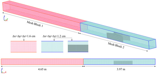
Figure 3.
Meshing configuration within the problem domain.
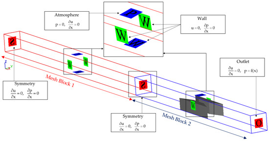
Figure 4.
Boundary conditions setup.
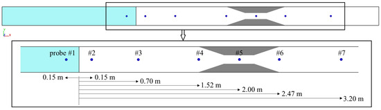
Figure 5.
Definitions of probe locations in the numerical model (where # indicates the probe number).
2.4. Verification of the Numerical Model
The validation and verification of the numerical model results were performed using water elevation data from the experiment conducted by Kocaman et al. [19]. The reason for choosing this parameter was the quantitative outputs that are needed for the current work. The meshing and accuracy of the numerical model should be sufficient to calculate the water level. In this process, the flow profiles were extracted within the range of 0 to 2.5 m downstream of the gate position at times 2.40 s, 4 s, and 5.50 s. Additionally, time-history water elevations at points p1, p3, and p5 were obtained. The verification process was carried out in three stages, as detailed in Section 2.4.1, Section 2.4.2 and Section 2.4.3.
2.4.1. Mesh Sensitivity Analysis
To analyze the meshing sensitivity, three numerical simulations with different mesh sizes, as detailed in Table 2, were conducted using RNG turbulence model. The mesh sizes had a refinement factor of 0.8 comparing two consecutive cases. The finest grid led to the generation of 848 × 103 cells, which increased the cell counts more than that result in cost-effective and relatively uneconomical numerical calculations. On the other hand, increasing the cell sizes more than Case 1 may result in unreliable outcomes. Therefore, the selected mesh sizes, as shown in Table 2, were considered reasonable and effective for determining the hydraulic parameters of this study. Flow profiles along the central plane of the channel and time-history water elevations were calculated, as shown in Figure 6 and Figure 7, respectively. The results indicate that the water elevation data for the three numerical models showed minimal variation (less than 1%), with the graphs nearly overlapping. This suggests that this parameter was not significantly sensitive to the selected mesh sizes. As seen in Table 2, reducing the mesh size from Case 2 to Case 3 increased the computational volume by 236% based on the number of cells, yet the accuracy of the water depth calculations remained largely unaffected. Conversely, despite the negligible difference in water elevation errors between Cases 1 and 2, the large cell size in Case 1 could cause substantial error in the calculation of other hydraulic parameters, such as the velocity field. Therefore, Case 2 is considered more reliable than Case 1. Given these findings, and in light of the expected results of this study, which includes both qualitative and quantitative water elevation data as well as velocity field observations, Case 2 was selected as the optimal mesh for this problem.
Table 2.
Specification of meshing used for the grid convergence analysis.
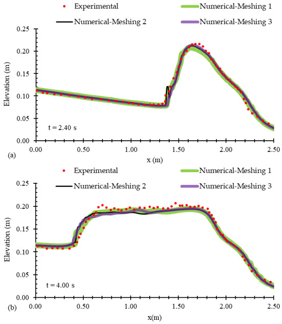
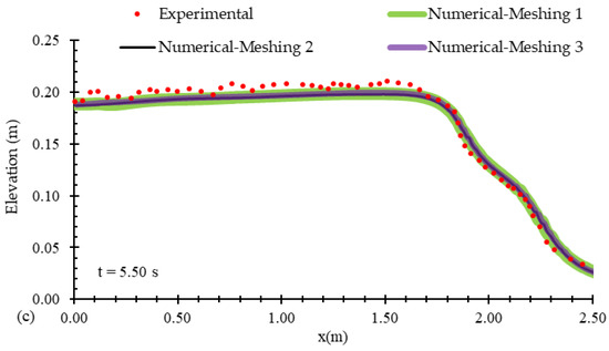
Figure 6.
Flow profiles calculated by numerical models with different mesh sizes, compared to the experimental data of Kocaman et al. [19], at times of (a) t = 2.40 s, (b) t = 4.00 s, and (c) t = 5.50 s after the gate removal.
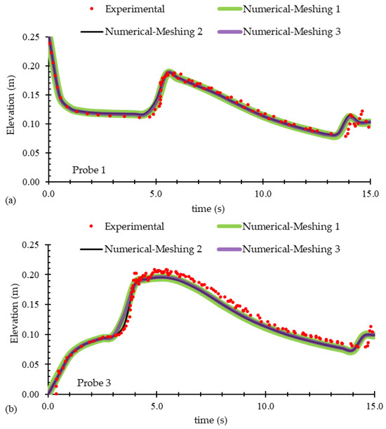
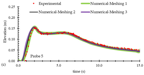
Figure 7.
Time-history water elevations calculated by numerical models with different mesh sizes, compared to the experimental data of Kocaman et al. [19], at three locations of (a) Probe 1, (b) Probe 3, and (c) Probe 5, as described in Figure 5.
2.4.2. Accuracy Comparison Between Turbulence Models
After adopting the optimal mesh, the reference model was applied to the three turbulence models: RNG, standard k-ε, and k-ω, to determine the most suitable model. To assess the accuracy of each one, flow profiles were evaluated at three time points: 2.40 s, 4.00 s, and 5.50 s. Figure 8 presents the result of the flow profile analysis at 4 s. The graphs of all three turbulence models show negligible difference, indicating that water elevation parameter was not sensitive to the choice of turbulence model in this problem. Considering the satisfactory performance of the RNG turbulence model in estimating a wide range of hydrodynamic parameters in hydraulic structure problems, specifically in dam-break simulations containing water–structure interactions [23,38,51,52,53,54,55,56,57], this model was selected for the numerical simulations in the present study.
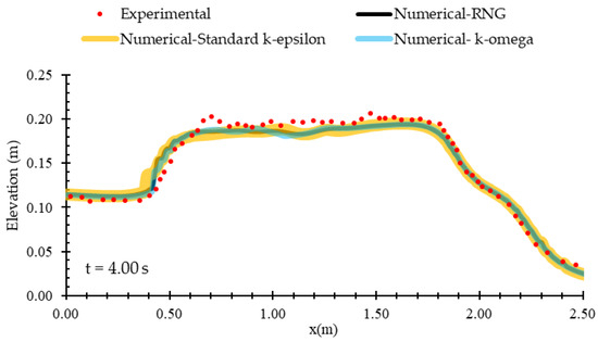
Figure 8.
Flow profiles with incorporation of three turbulence models in numerical calculations, compared to the experimental data of Kocaman et al. [19].
2.4.3. Accuracy Assessment of the Optimal Numerical Model
The accuracy of the optimal numerical model in comparison to the laboratory data was determined by calculating the Mean Absolute Percentage Error (MAPE), as defined by Equation (3):
In this equation, Xexp represents the experimental value, Xnum represents the numerical value, and n is the number of data points.
To calculate the error in the flow profiles (Figure 6), 15 points along the channel length on the central axis were selected for comparison. Water elevations at those points were compared between the numerical model outputs and the experimental data. This comparison was repeated for the three selected times in Figure 6. Additionally, to determine the percentage of error in the time-history elevations (Figure 7), water elevations at three selected points (p1, p2, and p3) were compared at 15 different times intervals, ranging from 1 s to 15 s after the event began.
3. Results
3.1. General Observations
The resulting average errors for the determination of flow profiles and time-history water elevations are represented in Table 3. Overall, the accuracy of the reference numerical model was calculated as 5.27% for the flow profiles and 5.59% for time-history water elevations, which is considered acceptable. Furthermore, the general observations of the numerical model results in Section 3.1, which indicate the satisfactory performance of the numerical model in describing the flow field, further confirm the accuracy of the outputs.
Table 3.
Mean Absolute Percentage Error (MAPE) of the numerical output compared to the experimental data of Kocaman et al. [19].
The flow profiles for the reference numerical run (as described in Figure 1) are plotted in Figure 9. As time progressed from the start of the event (the sudden removal of the gate), the dam-break wave reached the transition location, causing the water elevation increase at the converging point, as seen in Figure 9a. This increase in water elevation propagated upstream over time as a reflected wave, as observed in Figure 9b–d. It can be inferred that a hydraulic jump occurred at the transition point due to the collision between the high-velocity main flow and the slower-moving fluid. The formation of this initial hydraulic jump reduced the velocity and increased the water elevation upstream of the transition. Frequently, as the flow encountered upstream currents with low-velocity zones, hydraulic jumps were repeated. The position of this hydraulic jump shifted over time and moved upstream. The occurrence of a moving hydraulic jump was also evident in the Froude number contours presented in Figure 10. The Froude number in a vertical axis is defined as Fr = u. (g.h)−0.5, where u is the flow depth-averaged velocity at x direction, h is the average flow depth at corresponding axis, and g is gravitational acceleration. The flow coming from upstream initially had a Froude number greater than 1.0 and is considered supercritical. In open channels, for an approaching flow having a certain specific energy (h + v2/2g, where h is the flow depth and u is the flow velocity), the maximum discharge is achieved when the flow experiences the critical depth. When a supercritical flow encounters a narrower section, the flow depth across the transition increases, unless it reaches the critical depth. In that case, chocking occurs, and the water is repelled to gain the specific energy required to pass through the constriction at the critical depth. As a result, a hydraulic jump occurs, and the inflow changes from a supercritical state to a subcritical state [58]. This fact justifies the formation of the hydraulic jump during the initial times of collision between the incoming dam-break wave and the contractions shown in Figure 9, which can also be concluded in Figure 10 by observing the Froude number variations. Overall, the observation of the hydraulic response of a dam-break wave crossing the contraction align well with the experimental results of Kocaman et al. [19]. The response factors include time of flow choking and formation of hydraulic jump, water elevation rise at choking time, the reflected wave elevation, and the upstream propagation pattern of the reflected wave, which are obvious in Figure 9.
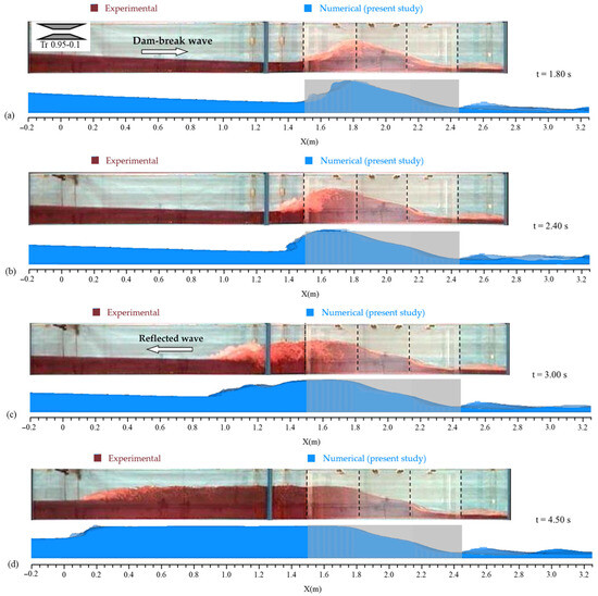
Figure 9.
Flow profiles for the reference case (present study) and experimental data [19] at times of (a) t = 1.80 s, (b) t = 2.40 s, (c) t = 3.00 s, and (d) t = 4.50 s after the gate removal.
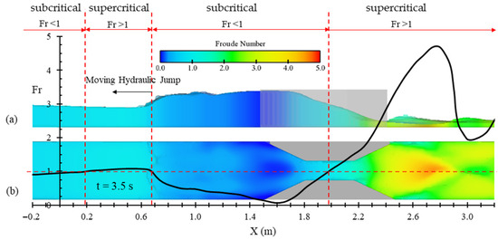
Figure 10.
Variation of the Froude number along the channel at the time of 3.5 s after the gate removal for the reference case: (a) sideview (across the channel’s centerline); (b) plan view.
The changes in the flow velocity at various times are demonstrated in the contours of Figure 11. The propagation state of the main flow as well as the hydraulic jump have reliable conformity with experimental results of Kocaman et al. [19]. At times 1.5, 1.8, and 2.1 s, the flow velocity at the transition site decreased. After 2.4 s, in the regions affected by the hydraulic jump, flow bifurcation became apparent, where the deeper parts of the flow exhibited a positive velocity (downstream direction) while the upper parts showed a negative velocity (upstream direction). Over time, the upper wave propagated upstream, and its speed gradually decreased. However, in the area affected by the reflected wave, the velocity of the main flow downstream decreased compared to the approaching flow due to the hydraulic jump. Upstream of the hydraulic jump, the velocity remained greater than 1.0 m/s in all cases. However, downstream of the hydraulic jump, the main flow velocity reduced to approximately 0.5 m/s. Meanwhile, the propagation velocity of the hydraulic jump (the upper wave velocity) initially reached a maximum of about −1 m/s and averaged around −0.5 m/s over time.
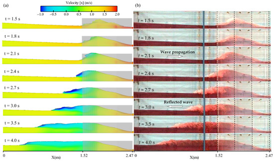
Figure 11.
(a) Contours of velocity field along the channel for the reference case (numerical results of present study); (b) corresponding flow profiles (experimental data [19]).
3.2. Effect of Transition Shape on Flow Hydraulics
According to Figure 2, four types of contraction shapes were tested along the channel path. To compare the effect of each transformation on the dam-break flow characteristics, the flow profiles were drawn at five different times, as shown in Figure 12. The profiles were extracted for the central plane (y = 0.15 m) and a lateral plane (y = 0.078 m) along the channel. For the cases tested in this section, the length of the transformation and the contraction width of the channel remained constant (L = 0.6 m and Lc = 0.1 m). It is worth noting that the cases of Tr 0.6–0.1 and Tr-C 0.6–0.1 had a triangle shape. As observed in Figure 12, the flow profiles for the central plane of the channel (y = 0.15 m) show that the water elevations in the range of x = 1.52 m to x = 2.12 m for both Tr-C and Cr-C states were zero, which is attributed to the presence of an obstacle in the flow path. Similarly, in the water surface profiles for the lateral plane (y = 0.078 m), the water levels were zero in the region where the flow encountered obstacles. Examining the flow profiles at times t = 1.0 s and t = 1.6 s (Figure 12a,b), it is clear that the profiles for the lateral transitions (Tr and Cr) followed a similar pattern, while the profiles for the obstacles in the center of the channel (Tr-C and Cr-C) followed a different pattern. At t = 1.6 s (Figure 12b), as the flow passed through the central obstacles, the water depth increased significantly along the central axis. However, over time, it became evident from the profiles at t = 2.0, 3.0, and 5.0 s (Figure 12c–e) that the reflected waves generated by the interaction of the flow with the trapezoidal obstacles (Tr and Tr-C) exhibited a consistent upstream propagation pattern. Similarly, the reflected waves associated with the crescent-shaped obstacles (Cr and Cr-C) followed a comparable pattern. In other words, from t = 2.0 s onward, the positioning of the obstacles no longer affected the reflected wave profile; instead, the wave profile was primarily determined by the shape of the obstacle. At t = 5.0 s (Figure 12e), the upstream wave elevation for the crescent-shaped transitions was approximately 1 cm (5.5%) greater than that of the trapezoidal obstacles. Moreover, the crescent-shaped contractions outperformed the trapezoidal ones in upstream wave propagation. Notably, in the four tested conditions shown in Figure 12, the maximum flow elevation at t = 5.0 s ranged between 19 and 20 cm, nearly filling the upstream distance up to the gate location (x = 0). This indicates that the reflected wave can elevate water elevations close to the initial reservoir level (25 cm) within 5 s of water release.
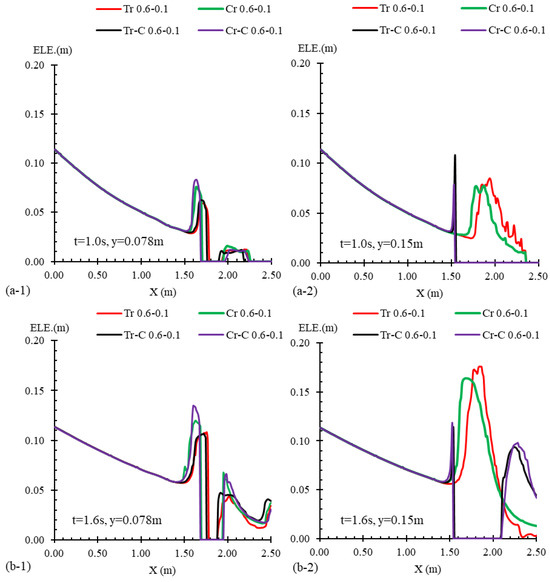

Figure 12.
Flow profiles for cases with different transition shapes, including Tr 0.6–0.1, Cr 0.6–0.1, Tr-C 0.6–0.1, and Cr-C 0.6–0.1, alongside the channel’s mid-width (y = 0.15 m) and quarter-width (y = 0.078 m) and at times of (a) t = 1.0 s, (b) t = 1.6 s, (c) t = 2.0 s, (d) t = 3.0 s, and (e) t = 5.0 s after the gate removal.
For a more detailed analysis of the effect of contraction shape on water elevations, their contours along the channel were extracted, as shown in Figure 13, for the four tested transformations with L = 0.9 m and Lc = 0.1 m. These configurations were longer than those in Figure 12, where L = 0.6 m. At first glance, the contours confirmed the three-dimensional nature of the flow, with water elevation varying across the transverse direction of the channel. At initial times (t = 2.0 s), the maximum flow depth was nearly 20 cm. In the cases with trapezoidal constrictions (Figure 13a,c), the water elevation extended over a larger area at the entrance of the contraction compared to the crescent ones (Figure 13b,d). This was due to the reduced disruption of streamlines in the crescent contractions, leading to less water accumulation. From t = 4.0 s onwards, the patterns of the wave for the crescent obstacle (Cr-C 0.9–0.1) and crescent contraction (Cr 0.9–0.1) became visually similar, as did those for the trapezoidal obstacle (Tr-C 0.9–0.1) and trapezoidal contraction (Tr 0.9–0.1), as noted in the water elevations. At t = 5.0 s, the reflected wave related to trapezoidal constrictions (Figure 13a,c) progressed upstream by about 0.2 m farther than the waves in the crescent configurations (Figure 13b,d), and, to some extent, the water elevations were also larger. The sharp edges of the trapezoidal contraction caused a more significant increase in water level during the initial stages of the dam-break flow collapse on the constriction, leading to a more progressive reflected wave. However, for the shorter transitions examined in Figure 12, the trapezoidal transformation with a length of 0.6 m formed a triangle in the flow path, which caused less convergence of flow lines compared to a trapezoidal alternative. As a result, the propagation pattern of the corresponding hydraulic jump differed between a triangle transition and a trapezoidal one.
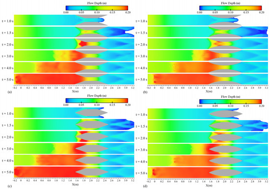
Figure 13.
Contours of the water elevation (flow depth) along the channel’s plan for cases with various contraction shapes, namely, (a) Tr 0.9–0.1; (b) Cr 0.9–0.1; (c) Tr-C 0.9–0.1; and (d) Cr-C 0.9–0.1.
In addition, the propagation of the wave alongside the velocity field in the central plane of the channel are presented in Figure 14 for four tested shapes of contraction with L = 0.95 m and Lc = 0.1 m. The propagation patterns complied with observations of the flow profiles and water elevation contours. In the area affected by the moving hydraulic jump, the flow bifurcation was observed for all tested conditions, where the upper flow layer had negative velocity and the lower part had positive velocity with small values, but there was not a significant pattern in comparing the concentrations of the two velocity zones between the four examined cases. The quantitative velocity interval of the reflected wave and also the main wave in the bottom in all subfigures of Figure 14 were similar for the four examined contractions, and the only difference was the propagation pattern. Faster propagation of the upstream wave in the cases of Tr and Tr-C was related to higher water elevations in t = 2.0 s (initial times as Figure 14a), as mentioned before. It is noticeable that at t = 2.0 s (Figure 14a), the flow exiting the contractions Tr and Cr had relatively larger velocity than the cases of Tr-C and Cr-C, because the water flowed downstream from the middle of the channel in the cases of Tr and Cr, not being obstructed by contractions.
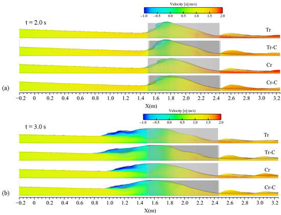
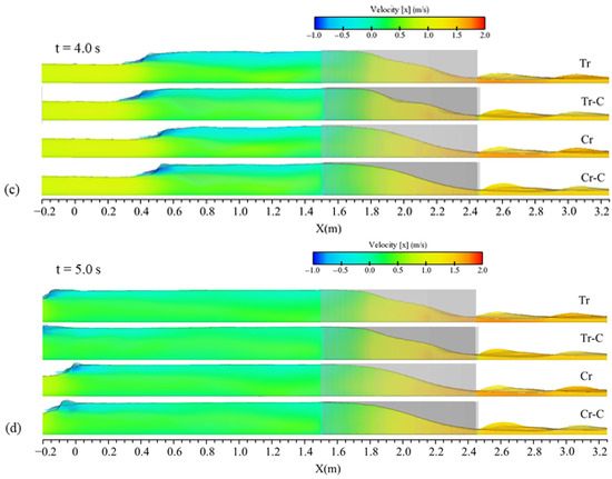
Figure 14.
Velocity contours alongside the flow profiles (side view) for cases with various contraction shapes, including Tr 0.95–0.1, Tr-C 0.95–0.1, Cr 0.95–0.1, and Cr-C 0.95–0.1 at times of (a) t = 2.0 s, (b) t = 3.0 s, (c) t = 4.0 s, and (d) t = 5.0 s after the gate removal.
3.3. Effect of Channel Contraction Width on Flow Hydraulics
Flow profiles for three cases including trapezoidal transitions of equal length (L = 0.9 m) but varying widths are presented in Figure 15. These profiles were observed along the central axis of the channel (y = 0.15 m) and a lateral axis at a quarter of the channel width (y = 0.078 m). The transitions were located between x = 1.52 m and x = 2.42 m. For the conditions tested, the channel widths at the transition point (Lc) were 0.1 m, 0.15 m, and 0.2 m corresponding to 33%, 50%, and 66% of the total channel width. The flow lines passing through the central axis (y = 0.15 m) did not encounter any of the transitions, while those passing through the lateral axis (y = 0.078 m (interacted with the Tr 0.9–0.1 transition. As a result, in a section of the channel that overlapped with the contraction, the water elevation was zero. From the initial seconds (t = 1.0 s and t = 2.0 s in Figure 15a,b), it was evident that greater contractions resulted in an increase in water elevation. The wave’s peak generated by the flow interacting with the transitions varied significantly across the different contraction conditions. At t = 2.0 s (Figure 15a), the wave’s peak at the central axis for the Tr 0.9–0.1 case was 20 cm. In contrast, for the Tr 0.9–0.15 and Tr 0.9–0.2 cases, these values decreased to 15 cm and 11 cm, respectively. This indicates that the transition with a larger contraction had a more significant effect on the water elevation. The streamlines passing through the larger contraction underwent a more substantial change in direction, resulting in greater energy dissipation and a higher accumulation of water entering the contraction. As a result, the water elevation increased. At t = 5.0 s (Figure 15c), the reflected waves in all three scenarios propagated upstream in a unidirectional pattern. The upstream water level in the case of Tr 0.9–0.1 reached 20 cm, whereas for the Tr 0.9–0.15 and Tr 0.9–0.2 cases, it decreased to 18 cm and 16 cm, respectively, at the central axis. In addition to the differences in the water elevation, the position of the wave front also varied among the three tested scenarios. At t = 5.0 s (Figure 15c), the wave fronts for the Tr 0.9–0.1, Tr 0.9–0.15, and Tr 0.9–0.2 cases were positioned approximately before the gate, 0.5 m downstream, and 1.1 m downstream of the gate, respectively. This indicates that the reflected wave formed by the dam-break flow encountering a more compact contraction travelled faster upstream, which resulted from larger water elevations at the entrance of the contraction at the initial times (t = 2.0 s). On the downstream side of the channel contraction (x > 2.47 m), the flow profiles followed a distinct pattern, as illustrated in Figure 15. In the initial seconds (t = 1.0 s and t = 2.0 s in Figure 15a,b), the flow profiles showed minimal variation, but over time, at t = 5.0 s, as shown in Figure 15c, the profiles diverged. At this point, the average water elevation downstream of the Tr 0.9–0.1 transition was 4 cm at axis y = 0.078 m, while downstream of Tr 0.9–0.15 and Tr 0.9–0.2 transitions, the average water elevations were 5 cm and 6 cm, respectively. Therefore, in contrast to the upstream reflected wave profile, the water elevation downstream of the transitions decreased as the contraction ratio increased.
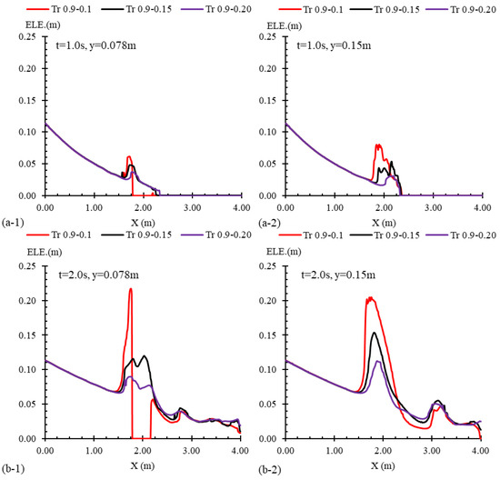
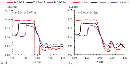
Figure 15.
Flow profiles for three cases with various contraction widths including Tr 0.9–0.1, Tr 0.9–0.15, and Tr 0.9–0.2 alongside the channel’s mid-width (y = 0.15 m) and quarter-width (y = 0.078 m) and at times of (a) t = 1.0 s, (b) t = 2.0 s, and (c) t = 5.0 s after the gate removal.
Furthermore, an analysis of the water elevation contours for the three cases is presented in Figure 16. It is observed that for all three Tr 0.9–0.1, Tr 0.9–0.15, and Tr 0.9–0.2 cases, in which the channel experienced 66%, 50%, and 33% compaction, hydraulic jump was present. In other words, in all cases, the approaching flow could not pass the transition without accumulating specific energy that led to the formation of hydraulic jump and a reflected progressive wave. For the case of Tr 0.9–0.1 (Figure 16a), the formation of the reflected wave was observed at t = 2.0 s, after the collision between the supercritical approaching flow with the channel contraction. The formation of the reflected wave was observed at larger times for the less compacted transitions. In the case of Tr 0.9–0.15 (Figure 16b) and Tr 0.9–0.2 (Figure 16c), the upstream wave started to propagate at t = 3.0 s and t = 4.0 s, respectively. This was because, in earlier times, the specific energy of the approaching supercritical flow could be large enough for passing the water during the contraction with higher water elevations without changing the flow regime to subcritical. However, due to unsteady water inflow, this equation could be changed, and the hydraulic jump would present at later times. Overall, Figure 16 reveals two key observations that comply with the flow profiles. Firstly, at similar times, the elevation of the hydraulic jump was greater when the flow interacted with a more converging transformation. Secondly, the hydraulic jump extended over a larger area upstream as the contraction increased.
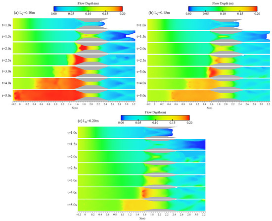
Figure 16.
Plan view of the water elevation (flow depth) contours for the three tested transitions with varying contraction widths: (a) Tr 0.9–0.1; (b) Tr 0.9–0.15; (c) Tr 0.9–0.2.
Figure 17 presents a comparison of velocity contours at four different time intervals for the three transition cases: Tr 0.9–0.1, Tr 0.9–0.15, and Tr 0.9–0.2. At t = 2.0 s (Figure 17a), an increase in water elevation was observed at the channel constriction for all three cases. However, the formation of a reflected wave was initially evident only in the Tr 0.95–0.1 case. Over time, flow bifurcation became noticeable upstream of the channel constriction, where velocity of the upstream wave, as shown in Figure 17b, approached approximately −1 m/s in the Tr 0.95–0.1 case. In the case of the transition with greater constriction, the upstream wave velocity was greater. The position of the upstream wave front varied among the three cases. At t = 4.0 s and t = 5.0 s (Figure 17c,d), the positions of the wave front differed by approximately 0.6 m, with the reflected wave in the most constricted transition advancing further upstream. The larger increase in water elevation at initial times (t = 2.0 s), along with the broader low-velocity zones at t = 5.0 s (Figure 17c,d), contributed to the intensification of the reflected wave originating from the more compact transition.
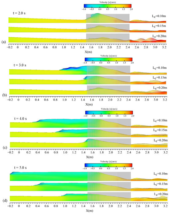
Figure 17.
Contours of longitudinal velocity along the channel for cases with different contraction ratios including Tr 0.9–0.1, Tr 0.9–0.15, and Tr 0.9–0.2 at times of (a) t = 2.0 s, (b) t = 3.0 s, (c) t = 4.0 s, and (d) t = 5.0 s after the gate removal.
3.4. Effect of the Transition Length on Flow Hydraulics
Flow profiles for three crescent-shaped transitions of varying lengths are depicted in Figure 18. In all cases, the channel width at the contraction section (Lc) remained constant at 0.15 m, while the transition lengths (L) were 0.6 m, 0.9 m, and 1.2 m. The flow lines passing through these transitions, both along the center axis of channel width (y = 0.15 m) and quarter-channel width (y = 0.078 m), did not directly interact with the transitions but rather passed in close proximity. Since all three transitions originated from the same position within the channel, the reflected waves within the first 2 s following gate failure (Figure 18a,b) had small differences in elevations, which was quite a bit higher for shorter transitions in the central axis. However, variations in the water elevation along the transition and downstream sections became more pronounced over time. By t = 5.0 s, as shown in Figure 18c, the reflected wave associated with Cr 0.6–0.15 advanced further upstream compared to Cr 0.9–0.15, showing a notable difference. Similarly, a comparable trend was observed for Cr 0.9–0.15 relative to Cr 1.2–0.15. The propagation of the hydraulic jump was linked to larger water elevations at the contraction site, which formed at the initial times. In the case of shorter contractions, the water elevations were slightly larger, contributing to a more pronounced reflection of the wave. Nonetheless, the differences in the reflected wave’s front remained subtle, and the water elevations remained nearly identical across all three cases. It is worth mentioning that at the contraction site, a notable increase in the water level was observed for the longer transition, which also influenced a greater longitudinal extent of the channel.
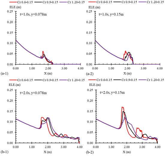
Figure 18.
Flow profiles for three cases with varied transition lengths, namely, Cr 0.6–0.15, Cr 0.9–0.15, and Cr 1.2–0.15, alongside the channel’s mid-width (y = 0.15 m) and quarter-width (y = 0.078 m) and at times of (a) t = 1.0 s, (b) t = 2.0 s, and (c) t = 5.0 s after the gate removal.
Contours of the water elevation for the same examined cases with varying contraction lengths are compared in Figure 19. At initial times, up to t = 2.0 s, the water elevation experienced a larger increase when the dam-break wave encountered a shorter transition (Figure 19a). At t = 2.0 s, the region of increased water level at the entrance of the Cr 0.6–0.15 case was wider than the Cr 0.9–0.15 case, and similarly, this area was wider for Cr 0.9–0.15 compared to Cr 1.2–0.15. The longer transitions featured softer edges that directed the flow lines downstream with a gentler slope, leading to less energy dissipation and a smaller velocity reduction at the contraction entrance, as well as a more modest increase in water elevation. In all three cases, the formation of the reflected wave caused by an initial hydraulic jump was evident, as shown in Figure 19. However, the start time of the upstream propagation differed by around 0.5 s between the cases. In the case of Cr 0.6–0.15 (Figure 19a), flow accumulation was observed at t = 2.0 s that led to an upstream wave observation at t = 2.5 s. Meanwhile, in the other two cases (Figure 19b,c), the flow chocking started at t = 2.5 s. This difference contributed to the lower convergence of the flow lines passing through the cases Cr 0.9–0.15 and Cr 1.2–0.15 than the case Cr 0.6–0.15. From t = 3.0 s onwards, differences in the location of the reflected wave became more apparent, with the position at t = 5.0 s differing by approximately 0.1 m between the three cases. These observations align with the flow profiles in Figure 18.
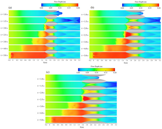
Figure 19.
Plan view of water elevation (flow depth) contours for three tested transitions with varying lengths: (a) Cr 0.6–0.15; (b) Cr 0.9–0.15; (c) Cr 1.2–0.15.
In addition, the propagation of the wave alongside the velocity field in the central plane of the channel is presented in Figure 20 for the same contractions with different lengths. The observed propagation patterns align with the results from the flow profiles and water elevation contours. In the region affected by the moving hydraulic jump, flow bifurcation was observed in all tested conditions, where the upper flow layer exhibited negative velocity and the lower part showed positive velocity with small magnitudes. However, there was no significant pattern when comparing the concentrations of the two velocity zones across the three examined cases. The quantitative velocity interval of the reflected wave and the main wave in the bottom in all subfigures of Figure 20 were almost similar for the three examined contractions, and the only difference was the propagation pattern. The faster propagation of the upstream wave in cases with shorter contractions was related to higher water elevations at t = 2.0 s as Figure 20a (initial times). This indicates that the shorter transitions resulted in a more rapid advance of the reflected wave due to the larger increase in water elevations in the earlier stages, which is justified in Figure 19.
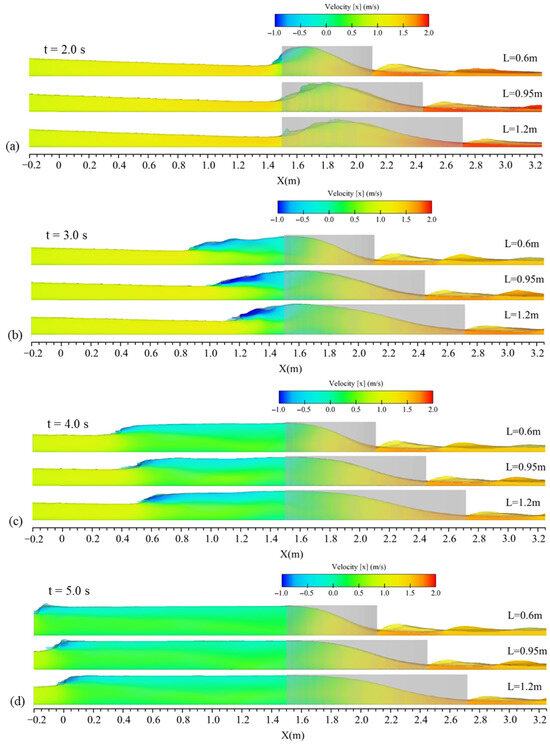
Figure 20.
Contours of longitudinal velocity distribution along the channel for cases with different contraction lengths including Cr 0.6–0.15, Cr 0.9–0.15, and Cr 1.2–0.15 at times of (a) t = 2.0 s, (b) t = 3.0 s, (c) t = 4.0 s, and (d) t = 5.0 s after the gate removal.
4. Discussion
The findings of this study provide important insights into the complex hydraulic behavior of unsteady flows triggered by sudden dam-break events in the presence of downstream geometric constrictions in a channel site. Water–structure interactions during a dam-break in a channel experiencing contraction was also investigated in a couple of previous studies [19,27,30,46], but in the present work, a reasonable geometric range of guide banks along an open channel was chosen for study, which adds a practical aspect to the present research. The results underscore the critical role of channel geometry, specifically the width and shape of contractions in shaping wave reflection patterns, hydraulic jump development, and upstream wave propagation. The considered constrictions included four arrangements of trapezoidal/crescent transitions at the middle of/across the channel. The tested contractions had widths of 66%, 50%, and 33% of the channel width and had lengths of twice, three times, and four times the channel width. The dam-break wave, caused by a sudden emptying of the reservoir, was set to collide with the transitions at a distance of six times the initial reservoir level (6h0). The results show that in all investigated channel contractions, the supercritical unsteady inflow could not cross the transitions without flow chocking and accumulation of water in the transition section. In all cases, formation of an initial hydraulic jump was observed that followed a reflected wave that propagated upstream by time; however, hydraulic jump (caused by flow choking) occurred at different times for different cases of contraction. Moreover, the water rise caused by the flow chocking at the transition section was different between cases. These two facts (time of flow choking and water elevation rise due to flow choking) were decisive in the progress of the hydraulic jump upstream.
Among the examined parameters, contraction width emerged as the most influential in generating hydraulic response. Higher contraction ratios led to stronger wave reflections and more significant upstream effects. The observation of flow profiles and water elevation contours showed that for three contractions occupying 66%, 50%, and 33% of the channel width (namely, Tr 0.9–0.1, Tr 0.9–0.15, and Tr 0.9–0.2, as described in Figure 2), dam-break flow crossing the transition choked at about t = 2.0 s, t = 3.0 s, and t = 4.0 s after the gate (dam) removal, respectively; meanwhile, the water elevations rose up to 20 cm, 15 cm, and 11 cm at the contraction site, respectively. By the formation of hydraulic jump and the reflected wave, the water elevation upstream of the contractions reached 20 cm, 18 cm, and 16 cm, respectively, for these cases at t = 5.0 s. These values for water elevations were extremely noticeable compared with the initial reservoir level (h0 = 25 cm). Additionally, observations on velocity contours in all the investigated cases indicated that in the area affected by hydraulic jump, flow bifurcation was evident where the upper flow layer had negative velocity (up to −1 m/s) and the bottom layer had positive velocity that was reduced due to being covered by hydraulic jump. Between the investigated cases, there was no significant difference between the velocity interval of the main flow or the reflected wave’s velocity. The main difference was the location of the upstream wave’s front at various times. At t = 5.0 s, the reflected wave fronts were positioned at x = −0.1 m, x = 0.5 m, and x = 1.1 m for Tr 0.9–0.1, Tr 0.9–0.15, and Tr 0.9–0.2, respectively (where x was measured from the initial gate location downstream). This proves that at a certain time, hydraulic response of the interaction between the dam-break wave and the higher-ratio contraction affected more of the area upstream. These quantitative comparisons are represented in Figure 21, providing a better conclusion about the hydraulic response of a dam-break wave interacting with guide-banks with various compaction ratios. In the diagrams of Figure 21, the water elevation (h) as well as downstream distance from the gate (x) parameters became dimensionless by being divided into the initial reservoir level (h0 = 25 cm); also, the time (t) parameter was multiplied by 0.01(g/h0)0.5 to become dimensionless (T = 0.01(g/h0)0.5 × t, where g is gravitational acceleration; for instance, T = 0.31 indicates the actual time of t = 5.0 s).
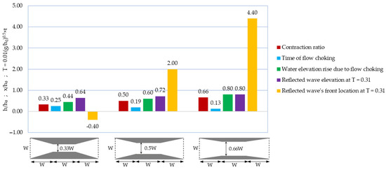
Figure 21.
Dam-break wave response interacting with the investigated guide-banks with various contraction ratios; transitions were located 6h0 downstream of initial gate location; W/h0 = 1.2.
The type of contraction shape (trapezoidal versus crescent) influenced the flow behavior differently. Trapezoidal geometries generated a more intense convergence of streamlines at the entrance, resulting in a slightly more progressive hydraulic jump, whereas crescent-shaped contractions led to smoother flow transitions. Comparing two cases, Tr 0.9–0.1 and Cr 0.9–0.1, the water elevation rise differed by 1 cm (0.04 times the h0) when it came to flow choking. Also, at t = 5.0 s, the reflected wave front in cases Tr 0.9–0.1 and Cr 0.9–0.1 were located at x = −0.2 m and x = 0, respectively; this fact further indicates the flow-line convergence effect on the upstream wave propagation. Following that, the contraction length did not directly affect the flow profiles, but the comparison between three crescent transitions with various lengths (namely, Cr 0.6–0.15, Cr 0.9–0.15, and Cr 1.2–0.15) revealed that the shorter transition led to more convergence of the approaching flow lines and therefore created a little more progressive hydraulic response. Moreover, the placement of the contraction (in the middle of/cross the channel) did not significantly cause different hydraulic responses. The comparison of water elevation variations between the Tr 0.9–0.1 and Tr-C 0.9–0.1 cases and also between Cr 0.9–0.1 and Cr-C 0.9–0.1 showed no significant difference in the maximum water rise by flow choking, the time of flow choking, and the propagation pattern of the hydraulic jump. In fact, the convergence of flow lines did not differ neither for Tr 0.9–0.1 and Tr-C 0.9–0.1 cases, nor between Cr 0.9–0.1 and Cr-C 0.9–0.1 cases.
This suggests that in the broader context of flood risk management and hydraulic infrastructure design, careful consideration of channel narrowing is essential to prevent undesirable hydraulic responses and potential damage upstream. These findings have practical implications for the design of energy dissipators, flow control structures, and flood conveyance systems where understanding the nature of reflected waves can inform safer and more efficient designs.
In a broader hydraulic and environmental engineering context, this research highlights the value of using calibrated numerical models to investigate transient flow phenomena with high spatial and temporal resolution. While experimental setups offer controlled observations, numerical tools allow for more extensive parametric explorations under variable and extreme conditions, which are often encountered in real dam-break scenarios.
Future research may expand on these findings by addressing several limitations identified in the current study. For instance, while sediment transport and erosion processes were not incorporated into the simulations, their inclusion is essential for capturing the long-term evolution of channel morphology and the feedback mechanisms that occur during real dam-break events. Additionally, this study only explored a limited range of geometric variations in channel constrictions, namely, specific trapezoidal and crescent- shaped configurations. Investigating a broader spectrum of structural forms, along with varying discharge conditions, would provide a more comprehensive understanding of dam-break hydraulics. Moreover, future work should examine the influence of channel roughness and wall material properties on wave reflection behavior, integrate three-dimensional flow simulations to capture shear stresses and turbulent structures more accurately, and assess the role of suspended materials typically mobilized during floods. Incorporating remote sensing or satellite-based data would also enable model validation across larger spatial domains with natural topographic complexity.
5. Conclusions
In the present study, the hydraulics of unsteady flow resulting from a sudden dam-break in a channel were investigated, with a focus on the interaction between the flow and various guide-bank transitions downstream. A numerical model was applied to estimate water elevations with acceptable accuracy based on experimental data from the literature. Incorporation of Reynolds-Averaged Navier–Stokes (RANS) equations for solving three-dimensional unsteady flow along with the Volume of Fluid (VOF) method for tracking the free surface reproduced the flow profiles and time-history water elevations with Mean Absolute Percentage Errors (MAPEs) of 5.27% and 5.59%, respectively. The model was used to determine flow profiles, analyze water elevation contours, and observe the flow velocity field for numerical cases containing modified guide-banks. The modifications included the shape of contraction (trapezoidal versus crescent), placement of guide-banks (laterally sides of channel versus in the middle of channel), widths of guide-banks, and lengths of guide-banks. The results show that for all cases, the incoming dam-break wave, which faced a contraction at a distance of 6h0 from the initial dam location (h0 = 0.25 m was the initial reservoir level), experienced flow choking with a hydraulic jump following a reflected wave upstream. However, the quantitative aspect of hydraulic response differed for the investigated cases. The determining factor was identified to be the convergence degree of flow lines across the transitions. Therefore, the width of the guide-bank was the most influential item. In the interaction between the dam-break wave with a more compact guide-bank, the time of flow choking was lesser; water elevation rise due to choking was higher; reflected wave elevation was larger; and at a certain time, it propagated more area upstream. Additionally, trapezoidal guide-banks led to more convergence of flow lines compared with crescent ones, therefore generating a noticeable larger response. The guide-bank placement and the length of it did not affect the hydraulic response as much as the convergence of flow lines remaining constant. Finally, quantitative hydraulic response parameters were extracted in a dimensionless form and presented in Figure 21 for three guide-banks with different width ratios. The results of this study have practical implications for predicting the dynamics of dam-break floods around downstream infrastructures, contributing to risk management and hazard analysis efforts. The findings can help improve our understanding of how various contraction geometries affect the propagation and intensity of reflected waves, ultimately aiding in better flood prediction and infrastructure design.
Author Contributions
Conceptualization, A.G. and H.S.; methodology, A.G., H.M. and H.S.; software, H.S., H.H. and J.H.P.; validation, A.G., H.S., H.M. and J.H.P.; investigation, A.G., H.M., H.M., H.H. and J.H.P.; resources, A.G.; data curation, A.G. and H.S.; writing—original draft preparation, A.G., H.M., H.M., H.H. and J.H.P.; writing—review and editing, A.G., H.M., H.M., H.H. and J.H.P.; supervision, A.G.; project administration, A.G.; funding acquisition, A.G. All authors have read and agreed to the published version of the manuscript.
Funding
This research received no external funding.
Data Availability Statement
The data are available to the corresponding authors upon reasonable request.
Conflicts of Interest
The authors declare no conflicts of interest.
Abbreviations
The following abbreviations are used in this manuscript:
| CFD | Computational fluid dynamics |
| RANS | Reynolds-averaged Navier–Stokes |
| SWE | Shallow-water equations |
| LES | Large eddy simulation |
| FVM | Finite volume method |
| VOF | Volume of fluid |
| FAVOR | Fractional Area/Volume Obstacle Representation |
| MAPE | Mean absolute percentage error |
| ELE | Elevation of water |
| Tr | Parallel lateral contraction with trapezoidal shape |
| Cr | Parallel lateral contraction with crescent shape |
| Tr-C | Parallel mid-width contraction with trapezoidal shape |
| Cr-C | Parallel mid-width contraction with crescent shape |
References
- Hamidifar, H.; Nones, M. Spatiotemporal variations of riverine flood fatalities: 70 years global to regional perspective. River 2023, 2, 222–238. [Google Scholar] [CrossRef]
- Merz, B.; Blöschl, G.; Vorogushyn, S.; Dottori, F.; Aerts, J.C.; Bates, P.; Bertola, M.; Kemter, M.; Kreibich, H.; Lall, U.; et al. Causes, impacts and patterns of disastrous river floods. Nat. Rev. Earth Environ. 2021, 2, 592–609. [Google Scholar] [CrossRef]
- Hamidifar, H.; Yaghoubi, F.; Rowinski, P.M. Using multi-criteria decision-making methods in prioritizing structural flood control solutions: A case study from Iran. J. Flood Risk Manag. 2024, 17, e12991. [Google Scholar] [CrossRef]
- Murtaza, N.; Pasha, G.A.; Hamidifar, H.; Ghani, U.; Ahmed, A. Enhancing flood resilience: Comparative analysis of single and hybrid defense systems for vulnerable buildings. Int. J. Disaster Risk Reduct. 2025, 116, 105078. [Google Scholar] [CrossRef]
- Wang, Y.; Fu, Z.; Cheng, Z.; Xiang, Y.; Chen, J.; Zhang, P.; Yang, X. Uncertainty analysis of dam-break flood risk consequences under the influence of non-structural measures. Int. J. Disaster Risk Reduct. 2024, 102, 104265. [Google Scholar] [CrossRef]
- Anjaneyulu, R.; Swain, R.; Behera, M.D. Future projections of worst floods and dam break analysis in Mahanadi River Basin under CMIP6 climate change scenarios. Environ. Monit. Assess. 2023, 195, 1173. [Google Scholar] [CrossRef]
- Yerramilli, S. Potential impact of climate changes on the inundation risk levels in a dam break scenario. ISPRS Int. J. Geo-Inf. 2013, 2, 110–134. [Google Scholar] [CrossRef]
- Hooshyaripor, F.; Tahershamsi, A.; Razi, S. Dam break flood wave under different reservoir’s capacities and lengths. Sādhanā 2017, 42, 1557–1569. [Google Scholar] [CrossRef]
- Najar, M.; Gül, A. Investigating the influence of dam-breach parameters on dam-break connected flood hydrograph. Tek. Dergi 2022, 33, 12501–12524. [Google Scholar] [CrossRef]
- Wang, B.; Zhang, J.; Chen, Y.; Peng, Y.; Liu, X.; Liu, W. Comparison of measured dam-break flood waves in triangular and rectangular channels. J. Hydrol. 2019, 575, 690–703. [Google Scholar] [CrossRef]
- Yu, M.-H.; Deng, Y.-L.; Qin, L.-C.; Wang, D.-W.; Chen, Y.-L. Numerical simulation of levee breach flows under complex boundary conditions. J. Hydrodyn. Ser. B 2009, 21, 633–639. [Google Scholar] [CrossRef]
- MacDonald, T.C.; Langridge-Monopolis, J. Breaching charateristics of dam failures. J. Hydraul. Eng. 1984, 110, 567–586. [Google Scholar] [CrossRef]
- Cao, Z.; Pender, G.; Wallis, S.; Carling, P. Computational dam-break hydraulics over erodible sediment bed. J. Hydraul. Eng. 2004, 130, 689–703. [Google Scholar] [CrossRef]
- Hogg, A.J.; Pritchard, D. The effects of hydraulic resistance on dam-break and other shallow inertial flows. J. Fluid Mech. 2004, 501, 179–212. [Google Scholar] [CrossRef]
- Oguzhan, S.; Aksoy, A.O. Experimental investigation of the effect of vegetation on dam break flood waves. J. Hydrol. Hydromech. 2020, 68, 231–241. [Google Scholar] [CrossRef]
- Feizi, A. Hydrodynamic study of the flows caused by dam break around downstream obstacles. Open Civ. Eng. J. 2018, 12, 225–238. [Google Scholar] [CrossRef][Green Version]
- Ismail, H.; Ann Larocque, L.; Bastianon, E.; Hanif Chaudhry, M.; Imran, J. Propagation of tributary dam-break flows through a channel junction. J. Hydraul. Res. 2021, 59, 214–223. [Google Scholar] [CrossRef]
- Lauber, G.; Hager, W. Experiments to dambreak wave: Sloping channel. J. Hydraul. Res. 1998, 36, 761–773. [Google Scholar] [CrossRef]
- Kocaman, S.; Güzel, H.; Evangelista, S.; Ozmen-Cagatay, H.; Viccione, G. Experimental and numerical analysis of a dam-break flow through different contraction geometries of the channel. Water 2020, 12, 1124. [Google Scholar] [CrossRef]
- Chen, Y.H.; Simons, D.B. An experimental study of hydraulic and geomorphic changes in an alluvial channel induced by failure of a dam. Water Resour. Res. 1979, 15, 1183–1188. [Google Scholar] [CrossRef]
- Goutiere, L.; Soares-Frazão, S.; Zech, Y. Dam-break flow on mobile bed in abruptly widening channel: Experimental data. J. Hydraul. Res. 2011, 49, 367–371. [Google Scholar] [CrossRef]
- Kocaman, S.; Ozmen-Cagatay, H. The effect of lateral channel contraction on dam break flows: Laboratory experiment. J. Hydrol. 2012, 432, 145–153. [Google Scholar] [CrossRef]
- Akgun, C.; Nas, S.S.; Uslu, A. 2D and 3D Numerical Simulation of Dam-Break Flooding: A Case Study of the Tuzluca Dam, Turkey. Water 2023, 15, 3622. [Google Scholar] [CrossRef]
- Biscarini, C.; Di Francesco, S.; Ridolfi, E.; Manciola, P. On the simulation of floods in a narrow bending valley: The malpasset dam break case study. Water 2016, 8, 545. [Google Scholar] [CrossRef]
- Haile, T.; Goitom, H.; Degu, A.M.; Grum, B.; Abebe, B.A. Simulation of urban environment flood inundation from potential dam break: Case of Midimar Embankment Dam, Tigray, Northern Ethiopia. Sustain. Water Resour. Manag. 2024, 10, 46. [Google Scholar] [CrossRef]
- Haltas, I.; Tayfur, G.; Elci, S. Two-dimensional numerical modeling of flood wave propagation in an urban area due to Ürkmez dam-break, İzmir, Turkey. Nat. Hazards 2016, 81, 2103–2119. [Google Scholar] [CrossRef]
- Xu, J.; Zhang, Y.; Ma, Q.; Zhang, J.; Hu, Q.; Zhan, Y. Dam-Break Hazard Assessment with CFD Computational Fluid Dynamics Modeling: The Tianchi Dam Case Study. Water 2025, 17, 108. [Google Scholar] [CrossRef]
- Hosseinzadeh-Tabrizi, S.A.; Ghaeini-Hessaroeyeh, M.; Ziaadini-Dashtekhaki, M. Numerical simulation of dam-breach flood waves. Appl. Water Sci. 2022, 12, 100. [Google Scholar] [CrossRef]
- Khoshkonesh, A.; Asim, T.; Mishra, R.; Dehrashid, F.A.; Heidarian, P.; Nsom, B. Study the effect of obstacle arrangements on the dam-break flow. Int. J. Comadem 2022, 25, 41–50. [Google Scholar]
- Kocaman, S.; Evangelista, S.; Guzel, H.; Dal, K.; Yilmaz, A.; Viccione, G. Experimental and numerical investigation of 3d dam-break wave propagation in an enclosed domain with dry and wet bottom. Appl. Sci. 2021, 11, 5638. [Google Scholar] [CrossRef]
- Di Cristo, C.; Greco, M.; Iervolino, M.; Vacca, A. Impact force of a geomorphic dam-break wave against an obstacle: Effects of sediment inertia. Water 2021, 13, 232. [Google Scholar] [CrossRef]
- Maghsoodi, R.; Khademalrasoul, A.; Sarkardeh, H. 3D numerical simulation of dam-break flow over different obstacles in a dry bed. Water Supply 2022, 22, 4015–4029. [Google Scholar] [CrossRef]
- Le, T.T.H.; Nguyen, V.C. Numerical study of partial dam–break flow with arbitrary dam gate location using VOF method. Appl. Sci. 2022, 12, 3884. [Google Scholar] [CrossRef]
- Oodi, S.; Gohari, S.; Di Francesco, S.; Nazari, R.; Nikoo, M.R.; Heidarian, P.; Eidi, A.; Khoshkonesh, A. Wave–Structure Interaction Modeling of Transient Flow Around Channel Obstacles and Contractions. Water 2025, 17, 424. [Google Scholar] [CrossRef]
- Beteille, E.; Larrarte, F.; Boyaval, S.; Demay, E.; Le, M.H. Dam-break flow over various obstacles configurations. J. Hydraul. Res. 2025, 63, 156–170. [Google Scholar] [CrossRef]
- Transportation Association of Canada. Guide to Bridge Hydraulics; Thomas Telford: Londen, UK, 2004. [Google Scholar]
- Chitale, S.V. Length and Shape of Guide Bunds. Water Energy Int. 1980, 37, 289–294. [Google Scholar]
- Ahmadi, M.; Ghaderi, A.; MohammadNezhad, H.; Kuriqi, A.; Di Francesco, S. Numerical investigation of hydraulics in a vertical slot fishway with upgraded configurations. Water 2021, 13, 2711. [Google Scholar] [CrossRef]
- Bayon, A.; Valero, D.; García-Bartual, R.; López-Jiménez, P.A. Performance assessment of OpenFOAM and FLOW-3D in the numerical modeling of a low Reynolds number hydraulic jump. Environ. Model. Softw. 2016, 80, 322–335. [Google Scholar] [CrossRef]
- Kocaman, S.; Ozmen-Cagatay, H. Investigation of dam-break induced shock waves impact on a vertical wall. J. Hydrol. 2015, 525, 1–12. [Google Scholar] [CrossRef]
- Mirkhorli, P.; Ghaderi, A.; Alizadeh Sanami, F.; Mohammadi, M.; Kuriqi, A.; Kisi, O. An investigation on hydraulic aspects of rectangular labyrinth pool and weir fishway using FLOW-3D. Arab. J. Sci. Eng. 2024, 49, 6061–6087. [Google Scholar] [CrossRef]
- Ozmen-Cagatay, H.; Kocaman, S.; Guzel, H. Investigation of dam-break flood waves in a dry channel with a hump. J. Hydro-Environ. Res. 2014, 8, 304–315. [Google Scholar] [CrossRef]
- Erduran, K.S.; Ünal, U.; Dokuz, A.Ş. Experimental and numerical investigation of partial dam-break waves. Ocean Eng. 2024, 308, 118346. [Google Scholar] [CrossRef]
- Launder, B.; Spalding, D.B. Turbulence modelling. Com. Mech. Appl. Mech. Eng. 1974, 3, 269. [Google Scholar] [CrossRef]
- Yakhot, V.; Orszag, S.A. Renormalization group analysis of turbulence. I. Basic theory. J. Sci. Comput. 1986, 1, 3–51. [Google Scholar] [CrossRef]
- Wilcox, D.C. Turbulence Modeling for CFD; DCW Industries: La Canada, CA, USA, 1998; Volume 2, pp. 103–217. [Google Scholar]
- Yang, S.; Yang, W.; Qin, S.; Li, Q.; Yang, B. Numerical study on characteristics of dam-break wave. Ocean Eng. 2018, 159, 358–371. [Google Scholar] [CrossRef]
- Issakhov, A.; Borsikbayeva, A. The impact of a multilevel protection column on the propagation of a water wave and pressure distribution during a dam break: Numerical simulation. J. Hydrol. 2021, 598, 126212. [Google Scholar] [CrossRef]
- Hirt, C.W.; Nichols, B.D. Volume of fluid (VOF) method for the dynamics of free boundaries. J. Comput. Phys. 1981, 39, 201–225. [Google Scholar] [CrossRef]
- Hirt, C.; Sicilian, J. A porosity technique for the definition of obstacles in rectangular cell meshes. In Proceedings of the 4th International Conference on Numerical Ship Hydrodynamics, Washington, DC, USA, 24–27 September 1985. [Google Scholar]
- Azimi, H.; Heydari, M.; Shabanlou, S. Numerical simulation of the effects of downstream obstacles on malpasset dam break pattern. J. Appl. Res. Water Wastewater 2018, 5, 441–446. [Google Scholar]
- Esmaeeli Mohsenabadi, S. Numerical Modeling of The Initial Stages of Dam-Break Problems. Ph.D. Thesis, Université d’Ottawa/University of Ottawa, Ottawa, ON, Canada, 2021. [Google Scholar]
- Ghaderi, A.; Abbasi, S.; Di Francesco, S. Numerical study on the hydraulic properties of flow over different pooled stepped spillways. Water 2021, 13, 710. [Google Scholar] [CrossRef]
- Ghaderi, A.; Dasineh, M.; Aristodemo, F.; Ghahramanzadeh, A. Characteristics of free and submerged hydraulic jumps over different macroroughnesses. J. Hydroinform. 2020, 22, 1554–1572. [Google Scholar] [CrossRef]
- Hien, L.T.T.; Van Chien, N. Investigate impact force of dam-break flow against structures by both 2d and 3d numerical simulations. Water 2021, 13, 344. [Google Scholar] [CrossRef]
- Rong, Y.; Zhang, T.; Peng, L.; Feng, P. Three-dimensional numerical simulation of dam discharge and flood routing in Wudu reservoir. Water 2019, 11, 2157. [Google Scholar] [CrossRef]
- Song, G.; Chen, Y.; Zhao, P.; Yuan, H. Numerical investigation on the evolutionary characteristics of landslide dam-break flow in a wet-bed channel with riparian vegetation. Front. Mar. Sci. 2024, 11, 1462760. [Google Scholar] [CrossRef]
- Te Chow, V. Open Channel Hydraulics Book; The Blackburn Press: Caldwell, NJ, USA, 2009; ISBN 07-010776-9. [Google Scholar]
Disclaimer/Publisher’s Note: The statements, opinions and data contained in all publications are solely those of the individual author(s) and contributor(s) and not of MDPI and/or the editor(s). MDPI and/or the editor(s) disclaim responsibility for any injury to people or property resulting from any ideas, methods, instructions or products referred to in the content. |
© 2025 by the authors. Licensee MDPI, Basel, Switzerland. This article is an open access article distributed under the terms and conditions of the Creative Commons Attribution (CC BY) license (https://creativecommons.org/licenses/by/4.0/).