An Interpretable Deep Learning Framework for River Water Quality Prediction—A Case Study of the Poyang Lake Basin

Abstract

Accurate prediction of water quality involves early identification of future pollutant concentrations and water quality indicators, which is an important prerequisite for optimizing water environment management. Although deep learning algorithms have demonstrated considerable potential in predicting water quality parameters, their broader adoption remains hindered by limited interpretability. This study proposes an interpretable deep learning framework integrating an artificial neural network (ANN) model with Shapley additive explanations (SHAP) analysis to predict spatiotemporal variations in water quality and identify key influencing factors. A case study was conducted in the Poyang Lake Basin, utilizing multi-dimensional datasets encompassing topographic, meteorological, socioeconomic, and land use variables. Results indicated that the ANN model exhibited strong predictive performance for dissolved oxygen (DO), total nitrogen (TN), total phosphorus (TP), permanganate index (CODMn), ammonia nitrogen (NH₃N), and turbidity (Turb), achieving R² values ranging from 0.47 to 0.77. Incorporating land use and socioeconomic factors enhanced prediction accuracy by 37.8–246.7% compared to models using only meteorological data. SHAP analysis revealed differences in the dominant factors influencing various water quality parameters. Specifically, cropland area, forest cover, air temperature, and slope in each sub-basin were identified as the most important variables affecting water quality parameters in the case area. These findings provide scientific support for the intelligent management of the regional water environment.

1. Introduction

Over the past few decades, global water quality has exhibited a consistent decline [1]. Anthropogenic activities have disrupted material cycling in water environments by altering land cover, intensifying point source emissions, and expanding non-point source pollution, making them the primary drivers of water quality deterioration [2]. Water quality prediction technology is a key tool in environmental governance, capable of elucidating spatiotemporal patterns of pollutant migration and transformation. Advancing water quality prediction research at the large watershed system level can aid in formulating region-specific water governance plans [3] and is essential for achieving the United Nations Sustainable Development Goal (SDG6) of “ensure availability and sustainable management of water and sanitation for all” [4].

As an integral component of water environment management, water quality prediction techniques have evolved markedly, shifting from traditional methods toward advanced machine learning approaches. Traditional prediction methods mainly include mechanistic and statistical approaches. Mechanistic models simulate pollutant transport, diffusion, and transformation processes based on hydrological, hydrodynamic, and physicochemical principles [5,6,7]. However, mechanistic models demand high data accuracy, complex parameterization, and exhibit low modeling efficiency [8]. Statistical models—including linear regression, logistic regression, and time series methods (e.g., ARMA, ARIMA)—typically assume linear relationships, constraining their capacity to capture nonlinear interactions between water quality changes and driving factors, thus restricting predictive accuracy [9,10,11,12,13].

The advancement of machine learning technology has introduced new approaches to addressing these challenges. Machine learning models, including neural networks, random forests, and support vector machines, efficiently process and analyze large-scale data by capturing complex patterns [14,15]. However, traditional machine learning models are less effective than deep learning models in processing large-scale, complex time series data [16]. As a subset of machine learning, deep learning models, with their multilayer architecture and strong ability to model nonlinear relationships, are crucial for improving the accuracy of water quality prediction [17,18]. Previous studies predominantly utilized recurrent neural networks (RNNs) and other time-series models to predict water quality based solely on historical water quality parameters, such as pH and dissolved oxygen [19,20,21]. In these studies, water quality parameters are both inputs and outputs for the models, while influencing factors such as climate, land use, and socioeconomic conditions are not considered. Consequently, these approaches result in black-box predictions with limited interpretability, hindering their effectiveness in elucidating causes of water quality variations and thus restricting their value for informed water management decisions.

Some researchers have integrated explanatory variables, such as precipitation and land use, to enhance model performance. For instance, Virro et al. [22] employed a random forest model combined with the Shapley additive explanations (SHAP) [23] method to analyze the influence of land use and meteorological factors on nitrogen and phosphorus pollution. However, their model exhibited systematic biases in predicting extreme concentrations and failed to consider the influence of socioeconomic factors on water quality. Soleymani et al. [24] applied machine learning models combined with the SHAP method to identify lake water level, water temperature, and inflow discharge as the primary environmental drivers of turbidity, without considering the potential impacts of land use and socioeconomic factors. Zheng et al. [25] proposed a climate–land use–socioeconomic deep learning framework that achieved variable importance analysis but did not include key geographic factors, such as watershed topographic slope, and failed to systematically assess the impact of different combinations of driving factors on predictive performance.

To address the limitations identified above, this study adopts an interpretable deep learning approach driven by multi-source datasets. The proposed approach integrates topographic information, meteorological time series, spatially explicit socioeconomic data (e.g., gross domestic product [GDP], population density), and high-resolution land use maps to construct a spatiotemporally coupled multilayer artificial neural network (ANN) model for predicting water quality. The model systematically elucidates mechanisms driving water quality variations influenced by both natural and anthropogenic factors, thereby providing robust scientific support for ecological governance in agricultural lake basins within the Yangtze River Economic Belt. This research addresses three primary objectives:

(1)

Developing an interpretable deep learning framework driven by multi-source data to enhance both predictive accuracy and model interpretability for water quality management in complex watershed systems.

(2)

Evaluating the effectiveness of multi-source data-driven collaborative deep learning methods in improving water quality prediction accuracy across large regions.

(3)

Investigating the explanatory variables that dominate the predictive performance of various water quality parameters and quantifying the contribution of key driving factors to water quality impacts.

2. Materials and Methods

2.1. Study Area

The Poyang Lake Basin (28°24′–29°46′ N, 115°49′–117°46′ E) is the largest interconnected lake basin in the middle and lower reaches of the Yangtze River, encompassing 162,200 km², or approximately 9% of the total Yangtze River Basin area (Figure 1). Of this area, 156,743 km² lie within Jiangxi Province, representing 96.62% of the entire basin [26]. The basin is connected to the Yangtze River via five major river systems: the Gan, Fu, Xin, Rao, and Xiushui Rivers. The average annual inflow into the Yangtze River accounts for 16.7% of its total runoff. The basin exhibits a distinctive “mountain-river-lake” topographic structure, characterized by surrounding mountains and a central alluvial plain around Poyang Lake. The subtropical humid monsoon climate yields an annual average precipitation of 1600–1900 mm and a mean temperature of approximately 17.5 °C [27]. Land use in the basin is primarily dominated by forestland and cropland. Industrialization, accompanied by rapid urbanization, has increased pressure on the water environment from human activities. Water quality is influenced by both natural hydrological cycles and human interference. During the flood season, nutrient concentrations increase markedly, exacerbating eutrophication trends in some lake areas. The shrinkage of natural wetlands and the decline in biodiversity have become prominent issues [28,29].

2.2. Data Sources and Preprocessing

The dataset used in this study includes water quality monitoring data, land use data, meteorological data, topographical data, and socioeconomic spatial data, covering the key environmental and socioeconomic dimensions of the case study area.

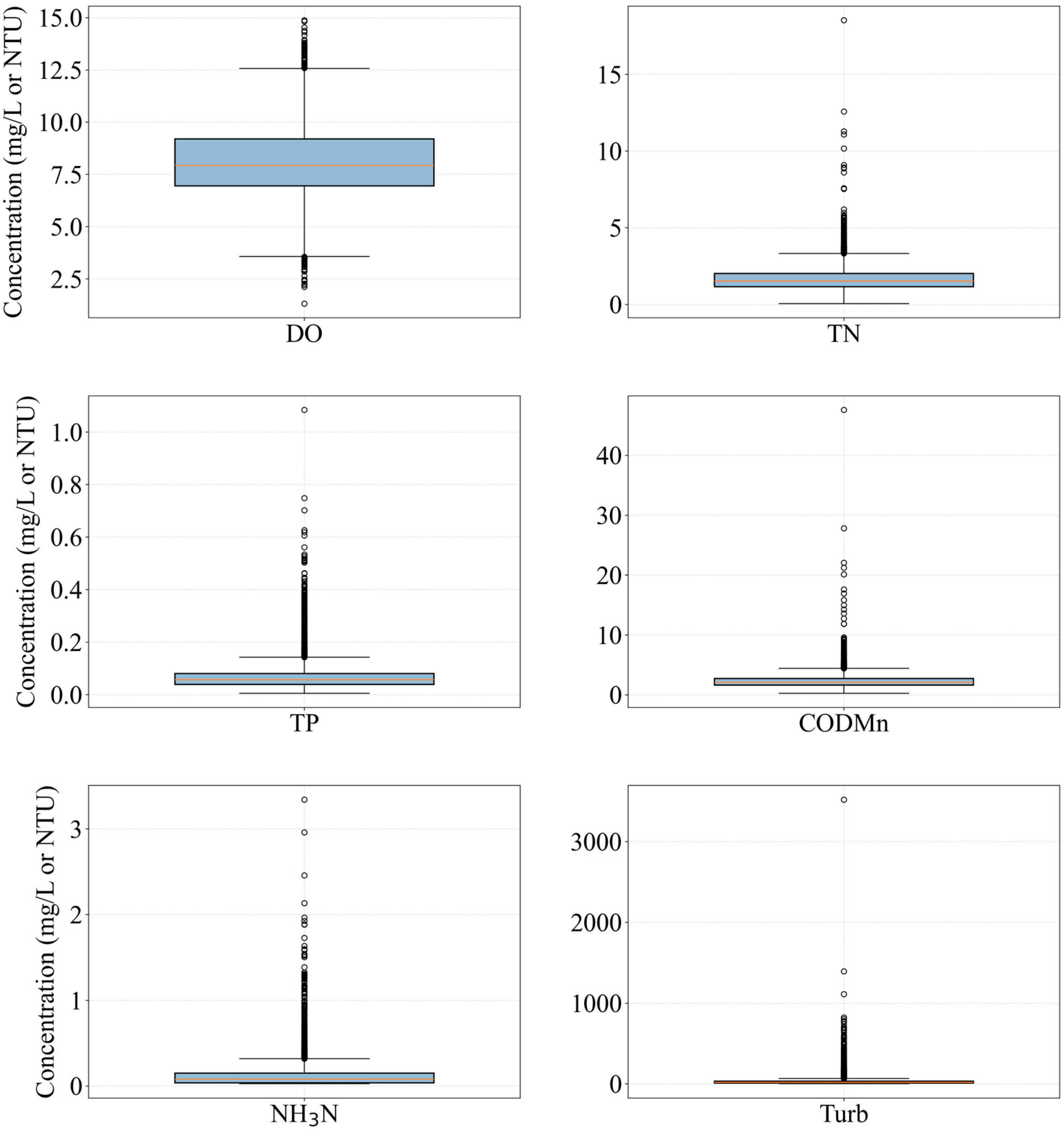
Water quality monitoring data were obtained from the real-time online dataset provided by China’s National Surface Water Quality Monitoring System from November 2022 to November 2023. A total of 22,515 water quality observations were obtained from 57 monitoring stations over a 395-day period, including both dry and wet periods as well as seasonal fluctuations throughout the year. All points shown in Figure 2 represent these 22,515 observations. The observed extreme values in the dataset primarily correspond to periods of major hydrological events (e.g., extreme rainfall or drought) and are also influenced by significant pollutant discharges from industrial and mining enterprises. The water quality parameters include total phosphorus (TP), total nitrogen (TN), ammonia nitrogen (NH₃N), dissolved oxygen (DO), permanganate index (CODMn), and turbidity (Turb). In this study, data from 57 monitoring sections in the case study area were selected. Each monitoring section corresponds to a section control unit, with both derived from the national control section setup and watershed division results during the “14th Five-Year Plan” period [30].

Meteorological data were obtained from the China National Meteorological Science Data Center. The study covers 63 meteorological stations, primarily providing daily precipitation and average temperature data. Based on previous studies [31,32], the following indicators were derived from daily precipitation data: total precipitation for the previous 3, 7, and 14 days and the number of days with precipitation less than 0.1 mm during the previous 7 and 14 days.

Land use data were obtained from the Environmental Systems Research Institute (Esri) [33] and are based on Sentinel-2 satellite imagery with a 10 m resolution, providing annual continuous data covering the period from 2017 to 2023. The data include nine land use types, from which six categories—water area, forest land, cropland, building land, bare land, and grassland—were selected as predictors of water quality based on their area proportions.

Socioeconomic data primarily include GDP, population density, and annual grain crop production as indicators of water quality. Annual grain crop production data were obtained from the Jiangxi Provincial Bureau of Statistics, GDP grid data from the published work of Deng et al. [34], and population grid data from the research of Huang [35].

The data preprocessing workflow for this study consists of three main steps: cross-sectional control units serve as the basic spatial units for data integration. Water quality data are processed by calculating the average concentration of multiple daily measurements from the same monitoring cross-section. Meteorological data are obtained by applying the shortest Euclidean distance method to match meteorological stations with target cross-sections, retrieving daily precipitation and temperature data synchronized with the water quality monitoring timestamps; Land use and socioeconomic data are extracted into cross-section control units using ArcGIS 10.8 tools. Grain production data are calculated based on cultivated land area and grain yield per unit area within the region. All factor data were normalized using the min–max method. Based on the box plot analysis for each water quality parameter (Figure 2), the parameters exhibit a skewed distribution. To optimize the distribution of water quality parameters, enhance the model’s sensitivity to low concentration values, and reduce the impact of extreme values, a logarithmic transformation was applied to the target variables.

2.3. Methodology

2.3.1. Research Framework

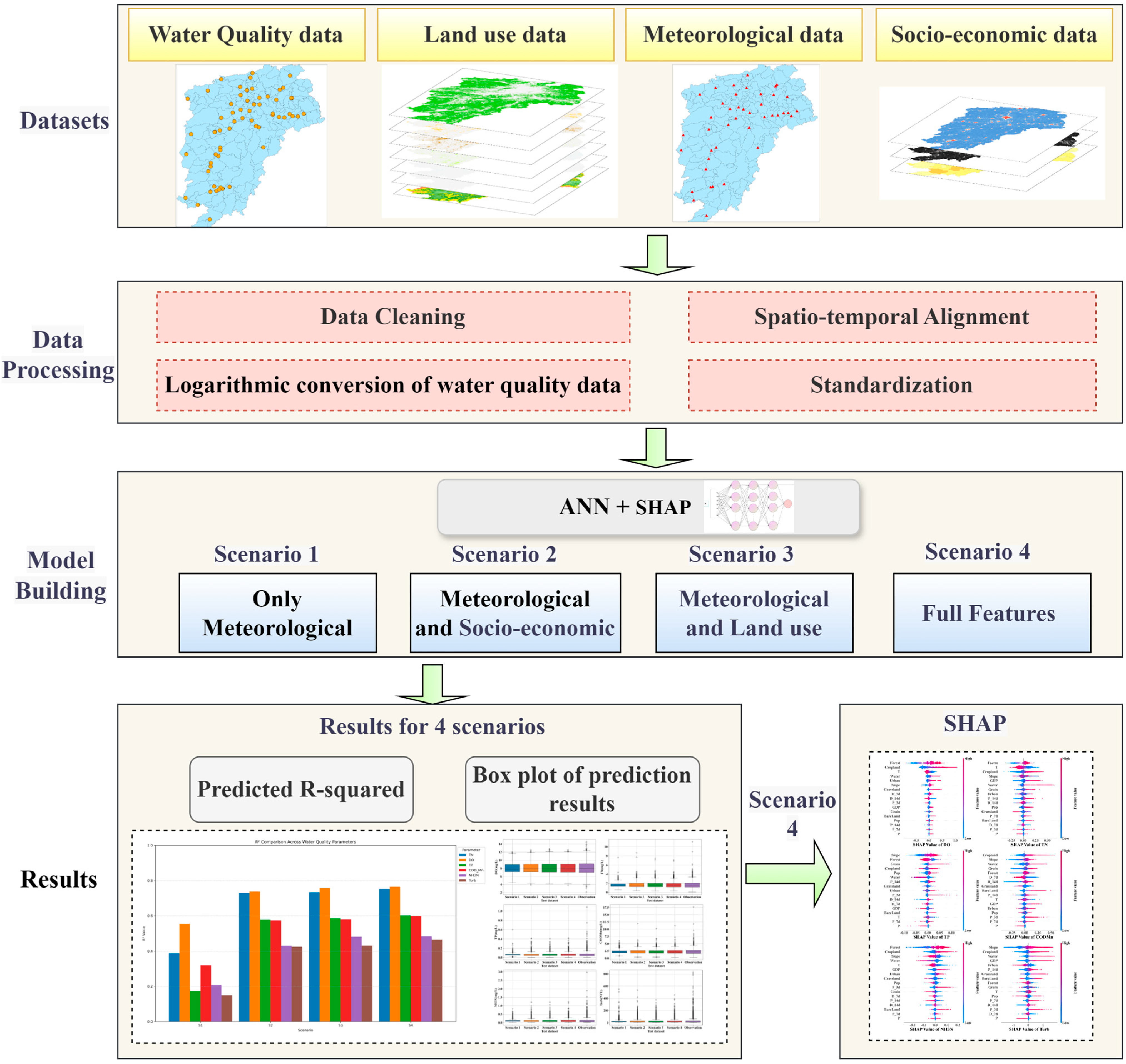
This study integrates deep learning modeling, multi-scenario comparative analysis, and interpretability to develop a watershed water quality prediction framework (Figure 3). The core process consists of the following:

Model design and experimentation: designing a three-layer feedforward neural network and constructing four scenarios based on meteorological, land use, and socioeconomic data; model evaluation: evaluating model performance (R², MSE) using 5-fold cross-validation and an independent test set and comparing the predictive accuracy of different scenarios; and model interpretability: using the SHAP method to analyze key drivers and their contributions.

2.3.2. Model Design

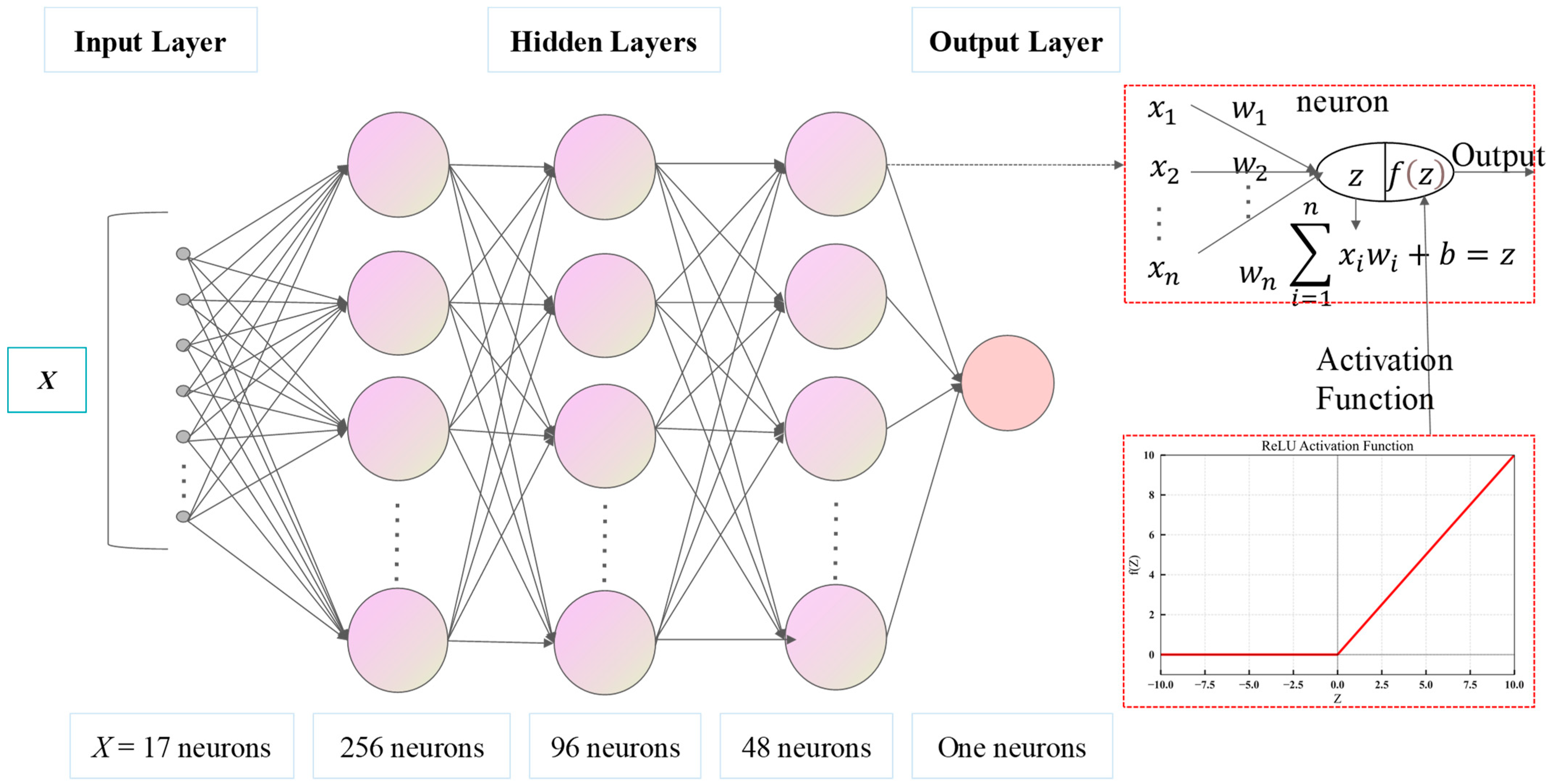
This study developed a model based on a multilayer feed-forward neural network to predict catchment water quality in the case area. The feed-forward neural network consists of three layers: an input layer, a multilayer hidden layer, and an output layer. These layers are connected by neurons, where the output of one neuron is passed as input to another neuron in the next layer [36]. The input data of each hidden neuron is first linearly combined with specific weights and biases. This combination is transformed into a nonlinear form within the neuron through an activation function. The data are processed through multiple layers until they reach the output layer.

This study developed a neural network model using the PyTorch 2.5.1 framework, consisting of an input layer, three hidden layers, and an output layer (Figure 4). The input layer contains 17 neurons, corresponding to 17 input variables, including slope, meteorology, land use, and socioeconomics. The three hidden layers contain 256, 96, and 48 neurons, respectively, all using the ReLU activation function [37] to introduce nonlinear transformations. The output layer applied a neuron with a linear activation function to generate the water quality parameters. The model was trained using the Adam optimizer, with a learning rate of 0.0015 and a training period of 150 epochs. The dataset was split into a training set and an independent test set in an 8:2 ratio. The model was trained using 5-fold cross-validation to enhance generalization and stability, with the final test result being the average of the predicted values from the 5 cross-validated models.

2.3.3. Model Training and Evaluation

Figure 5 displays the loss curves for both training and validation of the six water quality parameters. As the iteration steps increase, the mean squared error (MSE) decreases rapidly and then remains stable, indicating that the neural network model is convergent. Additionally, the MSE curve for the validation dataset closely follows that of the training dataset, indicating that no overfitting occurred during model training.

Each water quality parameter was individually input into the neural network model for prediction, with the untrained test set used to evaluate performance. Evaluation was performed using mean squared error, R², and median relative error. Figure 4 shows that the water quality distribution in the study area is skewed, indicating that most water quality parameters contain outliers or extreme values. To minimize the influence of outliers, the median, rather than the average, was used for relative error assessment, providing a more accurate reflection of the water quality prediction levels at each monitoring site [15]. The formula is as follows:

$$MSE={\displaystyle \frac{{\sum }_{i=1}^N{\left(y_i-{\tilde{y}}_i\right)}^2}{N}}$$

(1)

$$R^2=1-{\displaystyle \frac{{\sum }_{i=1}^N{\left(y_i-{\tilde{y}}_i\right)}^2}{{\sum }_{i=1}^N{\left(y_i-{\overline{y}}_i\right)}^2}}$$

(2)

$$MedianRelativeError=median\left(\left|{\displaystyle \frac{y_i-{\tilde{y}}_i}{y_i}}\right|\times 100\%\right)$$

(3)

where $y_i$ is a modeled water quality parameter,${\tilde{y}}_i$ is an observation, and ${\overline{y}}_i$ is the mean of the water quality data observations.

2.3.4. Modeling Scenarios

This study developed four scenarios and systematically integrated multi-source data, including meteorological elements, land use types, and socioeconomic indicators, to establish a system of explanatory variables for water quality prediction. Four sets of explanatory variable combinations were designed using the control variable method to assess the contribution of different driving factors to the water quality prediction model. A detailed summary of the modeling scenarios and their corresponding predictor variables is provided in

Table 1. Modeling of four scenarios for river water quality prediction in this study.

Modeling Scenarios	Predictor Variables
Meteorological Factor Coupling Scenario (S1)	Daily average temperature; daily precipitation; cumulative precipitation over the past 3 days, 7 days, and 14 days; and the number of dry days over the past 7 days and 14 days
Socioeconomic Expansion Scenario (S2)	S1 + GDP, population density, and grain production
Land Use Composite Scenario (S3)	S1 + cropland, forest land, water area, building land, bare land, and grassland
Multi-System Synergy Scenario (S4)	All factors

.

Recent research has demonstrated that economic development, population growth, industrial restructuring, and land use changes affect water resource consumption, pollutant emissions, and ecosystem service supply and demand [37,38,39]. The selection of socioeconomic and land use variables—such as GDP, population density, grain crop production, and land use structure—was based on extensive evidence that human activities play a crucial role in shaping water quality dynamics in river basins. That is, ignoring these factors would underestimate the impact of anthropogenic drivers on water quality.

2.3.5. Model Interpretability

In this study, the Shapley additive explanations (SHAP) framework [23], based on game-theoretic Shapley values, was used to quantitatively assess the independent and interactive contributions of meteorological, land use, and socioeconomic variables to the water quality prediction model. The SHAP methodology follows Lloyd [40] Shapley’s axiomatic system of fair allocation for coalitional games proposed in 1953 and centers on constructing additive explanatory models of feature contributions that satisfy the criteria of Local Accuracy, Missingness, Consistency, and Interaction. The core idea of the SHAP value is derived from the fair allocation principle in cooperative game theory, measuring the strength of its influence on model output by calculating the average marginal contribution of a feature across all subset combinations. Specifically, the SHAP value ${\mathrm{\varnothing }}_i(f,x)$ of a feature i is defined as follows:

$${\varnothing }_i\left(f,x\right)=\sum _{S\subseteq F\left\{i\right\}}{\displaystyle \frac{\left|S\right|!\cdot \left(\left|F\right|-\left|S\right|-1\right)!}{\left|F\right|!}}\left[f_{S\cup \left\{i\right\}}\left(x_{S\cup \left\{i\right\}}\right)-f_S\left(x_S\right)\right]$$

(4)

where:

-

$F$ is the full set of features (e.g., climate, land use, socioeconomic variables), and $S$ is an arbitrary subset without features;

-

$f_{S\cup \left\{i\right\}}$ is the model containing feature i, and $f_S$ is the control model excluding features;

-

$x_S$ denotes the feature values in the input vector $S$ that retain only a subset of features.

Compared to traditional feature importance ranking methods, the SHAP framework offers the following advantages: (1) directional sensitivity: distinguishing the promoting and suppressing effects of variables on water quality deterioration using positive and negative SHAP values; (2) sample-level interpretation: generating feature contribution maps for individual samples to reveal the dynamic evolution of dominant factors in specific hydrological conditions.

3. Results

3.1. Accuracy Assessment and Comparison of Water Quality Prediction Under Different Input Scenarios

The accuracy of water quality predictions varies significantly across different input scenarios (

Table 2. Mean squared error (MSE) and coefficient of determination (R²) of water quality predictions obtained using the test dataset. Dissolved oxygen, DO; total nitrogen, TN; total phosphorus, TP; permanganate index, CODMn; ammonia nitrogen, NH₃N; turbidity, TURB.

Indicators	Scenario	TN	DO	TP	CODMn	NH3N	TURB
R2	S1	0.388	0.555	0.174	0.320	0.208	0.150
	S2	0.730	0.738	0.579	0.574	0.430	0.425
	S3	0.734	0.758	0.587	0.581	0.481	0.431
	S4	0.754	0.765	0.603	0.599	0.484	0.465
MSE	S1	0.292	1.108	0.002	0.609	0.012	1802.509
	S2	0.132	0.622	0.001	0.388	0.009	1219.684
	S3	0.127	0.603	0.001	0.379	0.008	1206.893
	S4	0.126	0.572	0.001	0.367	0.008	1135.663

). The baseline scenario (S1) yields R² values between 0.1 and 0.4, reflecting weak predictive performance. This is largely attributable to the reliance solely on meteorological variables, which offer limited explanatory power. In addition, the short duration of available meteorological records may restrict the model’s capacity to capture temporal variability, thereby further reducing its predictive accuracy. The comprehensive scenario (S4), which integrates meteorological factors, land use, and socioeconomic variables, shows higher prediction accuracy than the other three scenarios. Specifically, scenario S4 showed relative improvements in R² values ranging from 37.8% to 246.7%, clearly reflecting significant performance enhancement compared to baseline scenario S1; for MSE, it showed a reduction in prediction error of 33.3% to 56.8% compared to S1. Compared with scenarios S2/S3, the accuracy of scenario S4 is slightly improved. For example, for TN, S4 is 3.4%/2.8% higher than S2/S3; for TP, it is 4.3%/2.8% higher; for CODMn, it is 4.4%/3.1% higher; for NH₃N, it is 12.7%/0.7% higher; and for turbidity, it is 9.3%/7.8% higher. For all water quality indicators, S3 accuracy is slightly higher than S2 but higher than S1. TN accuracy for S2/S3 is over 88% higher than S1; TP accuracy for S2/S3 is 230% higher than S1; and the S2/S3 values for CODMn and NH₃N increased by over 80% and 130%, respectively, compared to S1. The S2/S3 values for turbidity (Turb) increased by over 180% compared to S1.

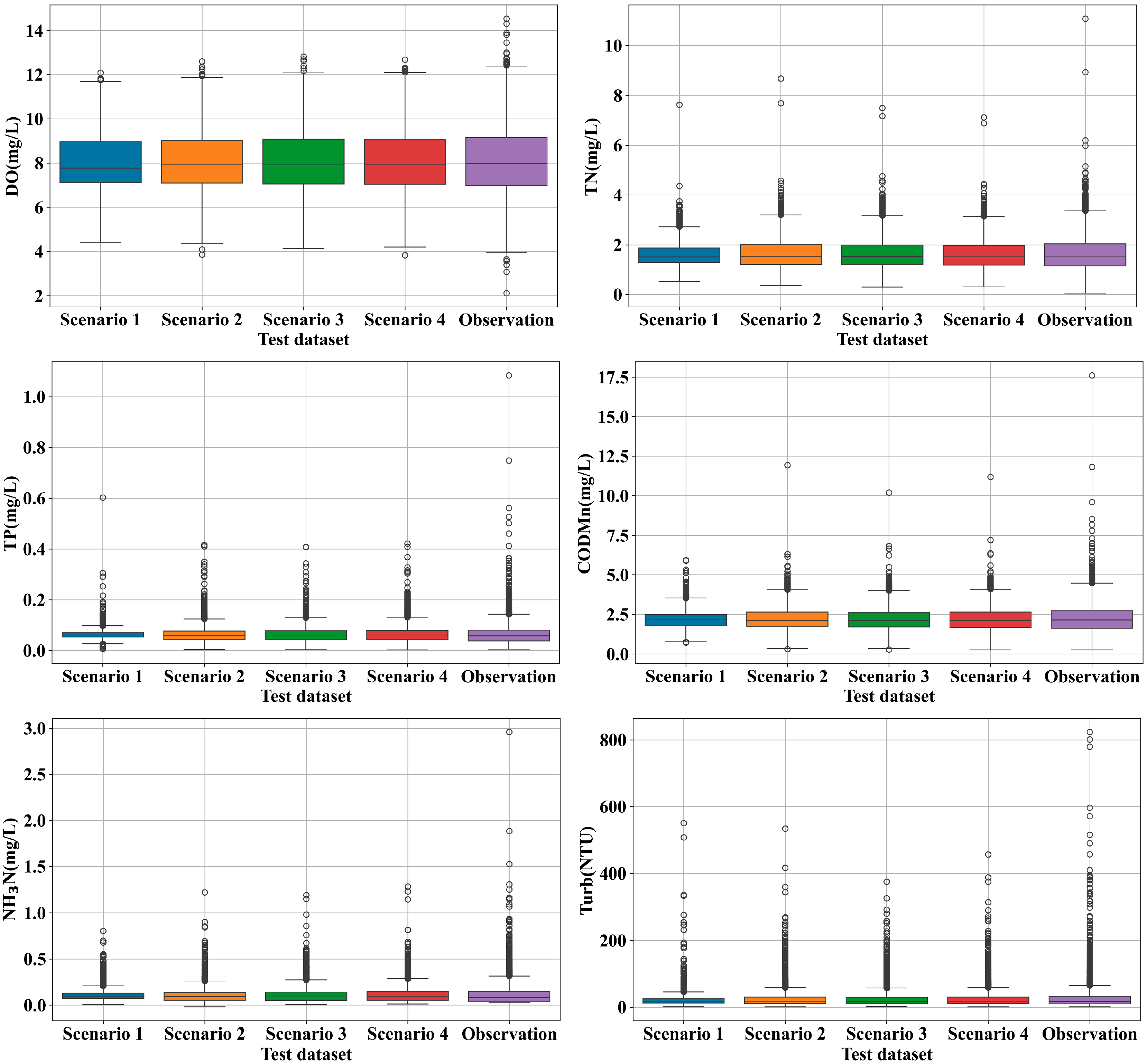
Box plots were further used to compare the distribution characteristics of predicted values across different input scenarios (Figure 6). The results showed that, according to both the R² metric (Table 2) and the closeness of medians and quartiles in the box plots, the all-factor scenario (S4) most closely matches the measured values, with the smallest difference in medians and reduced data dispersion compared to single-factor scenarios. Although the visual differences between scenarios in Figure 6 may appear small, S4 demonstrates superior predictive performance as indicated by higher R² values and a closer alignment with observed distributions across the median, first quartile (Q1), and third quartile (Q3) of water quality parameters. This improvement reflects the benefit of integrating multiple variable groups, rather than simply increasing the number of parameters. For clarity, “closest” here refers to both statistical alignment in distribution (median, Q1, Q3) and improved overall R² compared with the other scenarios.

These results indicate that the synergistic integration of multi-source meteorological, land use, and socioeconomic variables notably improves water quality prediction accuracy. Land use and socioeconomic factors are indispensable for water quality prediction, with land use variables having a slightly greater influence on water quality parameters than socioeconomic variables. Based on this, the subsequent analysis focuses solely on the results of the all-factor scenario.

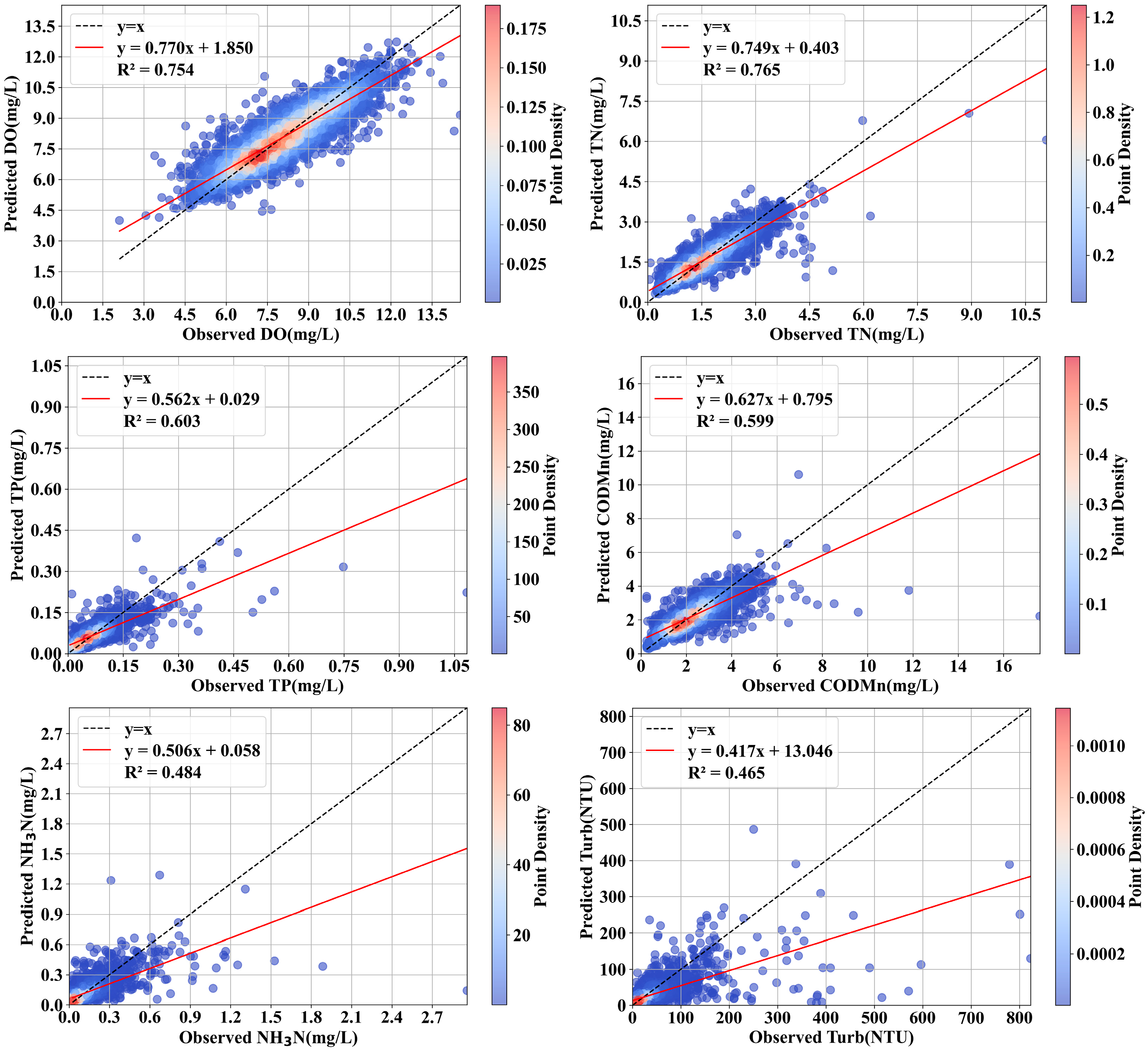
Figure 7 illustrates the relationship between the predicted and true values of the six water quality indicators under the all-factor scenario. The results show that dissolved oxygen (DO) and total nitrogen (TN) are better predicted, with the data points more tightly clustered around the diagonal line and higher R² values (0.75 and 0.77, respectively), indicating high prediction accuracy for these indicators. In contrast, permanganate index (CODMn) and total phosphorus (TP) also demonstrate strong linear relationships, but their data points are more dispersed with lower R² values (0.60). Ammonia nitrogen (NH₃N) and turbidity (Turb) were poorly predicted, with large outliers and low R² values (0.48 and 0.47, respectively). To statistically confirm the significance of these relationships, a regression-based analysis of variance (ANOVA) was conducted for each water quality parameter. As shown in

Table 3. ANOVA results for regression between observed and predicted values for each water quality parameter. Dissolved oxygen, DO; total nitrogen, TN; total phosphorus, TP; permanganate index, CODMn; ammonia nitrogen, NH₃N; turbidity, Turb.

Parameter	F_Value	p_Value
DO	14,700.89	<0.001
TN	14,821.96	<0.001
TP	6950.57	<0.001
CODMn	6976.23	<0.001
NH3N	4150.01	<0.001
Turb	3799.31	<0.001

, all models yielded extremely high F-values (ranging from 3799.31 to 14,821.96) and highly significant p-values (p < 0.001), indicating that the relationships between predicted and observed values are robust and statistically significant.

3.2. Spatial Differences in Water Quality Prediction Accuracy

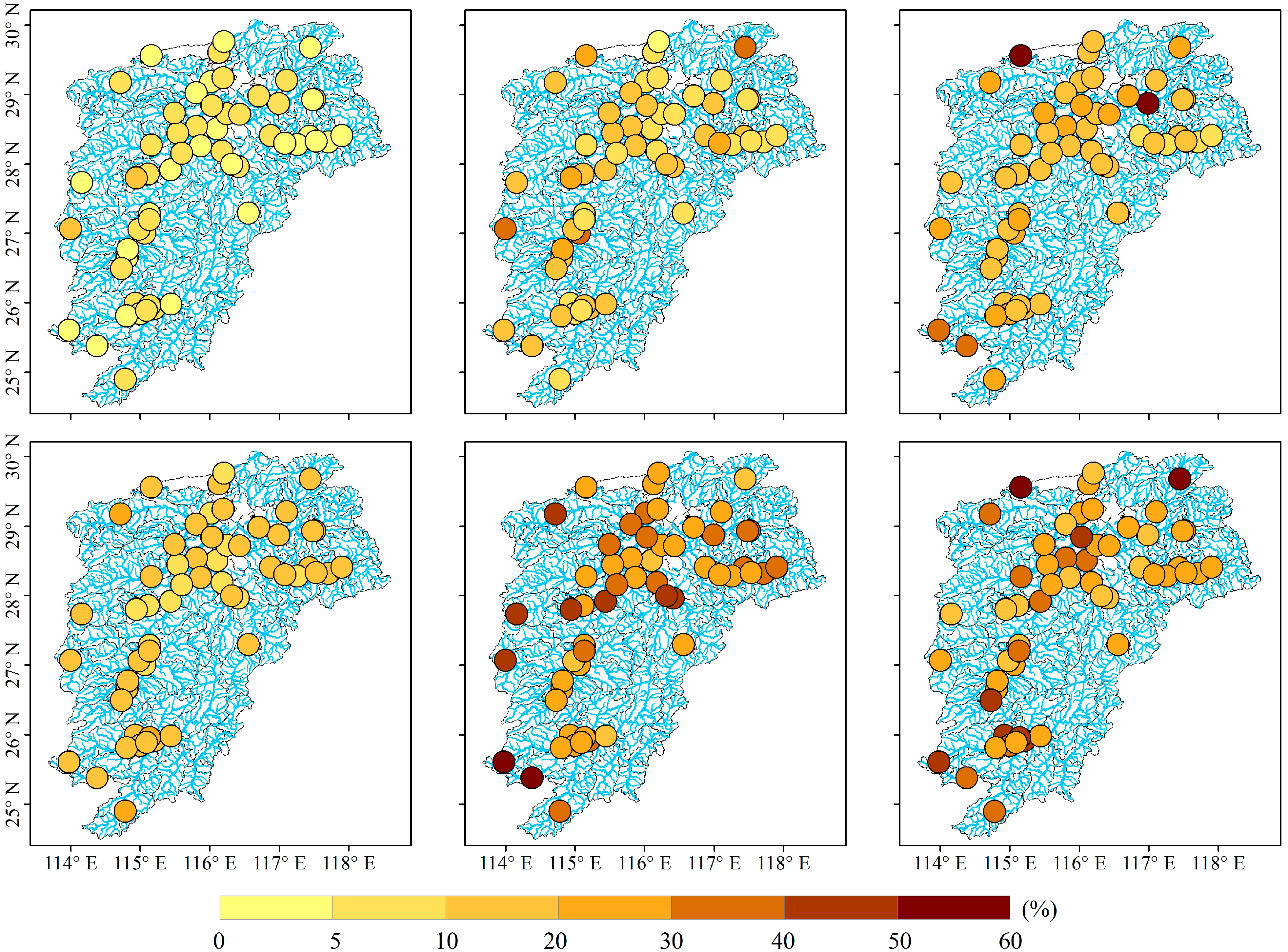
In all-element scenarios, the prediction results (Figure 8) show that the relative error for DO ranges from 2.66% to 11.34%, with a few sites in the western part of the study area exhibiting a fitting error below 10%. The relative error for TN ranges from 4.46% to 23.30%, with high values scattered across the western and northern parts of the study area. The relative error for TP ranges from 7.38% to 53.04%, with high values primarily in the Gan Nan region of the upper Gan River and its tributaries near the Yangtze River. The relative error for CODMn ranges from 5.76% to 21.80%, with better fitting results in the middle and lower reaches of the Gan River. The relative error for NH₃N ranges from 16.66% to 51.91%, and for Turb, it ranges from 12.67% to 57.63%. The overall fitting performance for both is poor, with errors generally exceeding 20%, especially in the southern part of the study area. Monitoring stations in the northern Poyang Lake basin are relatively concentrated, with smaller relative errors for the six water quality predictions in this region. However, the overall prediction performance of stations at the basin edges is poor, and most of these stations are located in the upstream region. This may be due to the surrounding stations being sparsely distributed, making it difficult for the model to fully learn the influence of basin characteristics on water quality. The relative errors are higher in the lake inlet and river mouth areas of the basin, particularly at the Poyang Lake inlet and the middle and lower reaches of the Ganjiang River basin. This may be due to the complex mixing process of tributaries with different water qualities when merging with the main river, making it challenging to predict the comprehensive water quality in the convergence zone.

The analysis indicates that high error values are mainly concentrated at the source and downstream confluence points. The source area has sparse monitoring stations, making it difficult for the model to fully learn the impact of watershed characteristics on water quality. The middle and lower reaches feature large water volumes, complex and diverse pollution sources, and intricate mixing and dilution processes, making it difficult for the model to accurately predict comprehensive water quality at the confluence.

3.3. Driving Forces of Water Quality

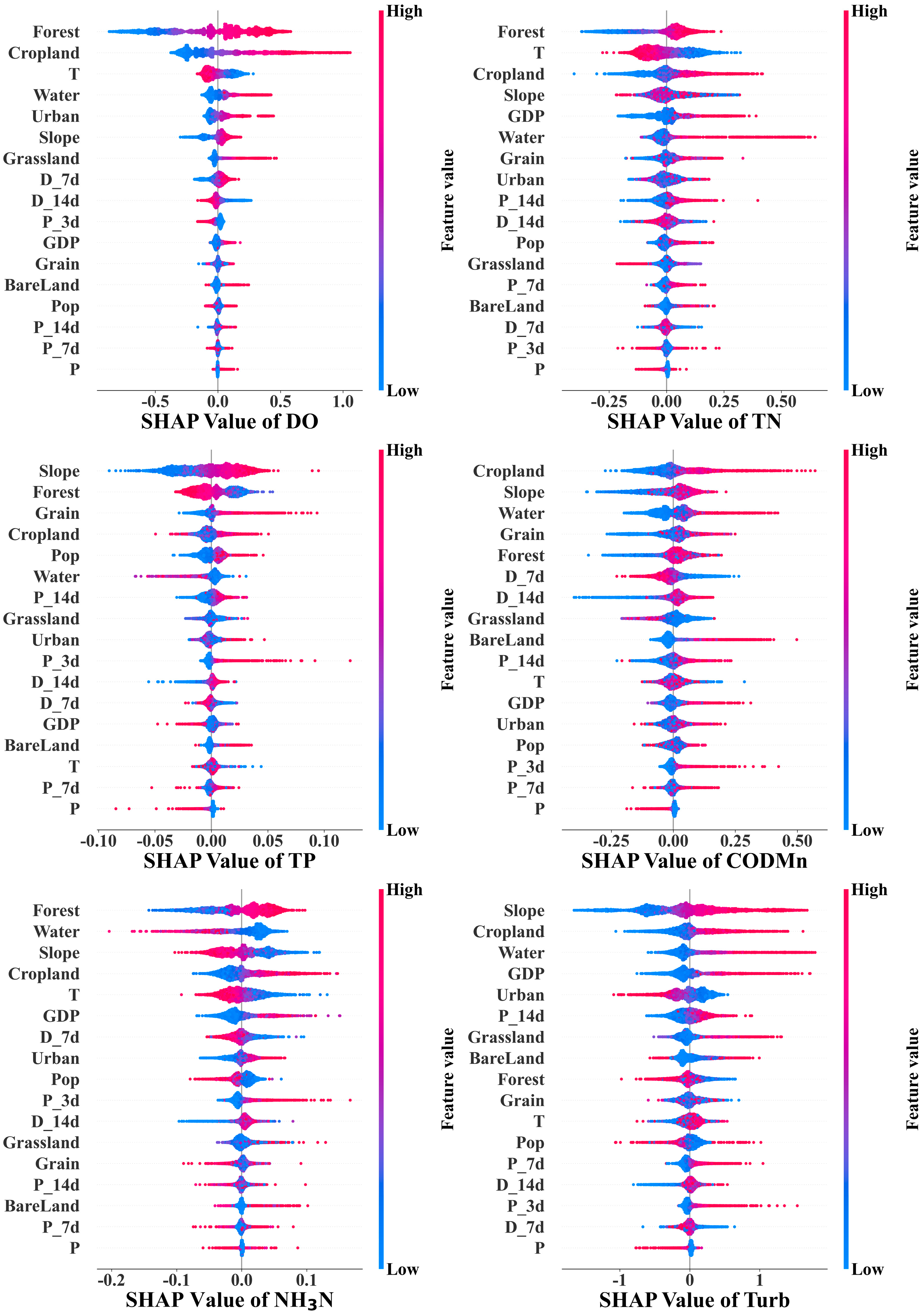
Through SHAP analysis of each model, the importance of meteorological factors, land use types, and socioeconomic factors on each water quality parameter was calculated, as shown in Figure 9. For each parameter, variables were ranked by their mean absolute SHAP value, with higher values indicating a greater contribution to the model output. In this analysis, a variable was considered to have a “significant impact” if it was consistently ranked among the top five predictors (by mean absolute SHAP value) for a given water quality indicator. The same criterion was used to identify other influential variables for each indicator. Forest land, cropland, air temperature, water area, and building land are the main variables affecting dissolved oxygen concentration. In contrast, the main factors affecting total nitrogen concentration include forest land, air temperature, cropland, slope, and GDP. The main variables affecting total phosphorus concentration are slope, forest land, grain crop yield, cropland, and population density; the main factors affecting permanganate concentration are cropland, slope, water area, grain crop yield, and forest land; ammonia nitrogen concentration is affected by forest land, water area, slope, cropland, and air temperature; and turbidity is mainly affected by slope, cropland, water area, GDP, and building land. The above results show that the main factors affecting water quality are land use and socioeconomic variables. Notably, cropland appeared among the top five most important variables for all six water quality parameters, highlighting its consistent and strong influence across indicators. Meteorological variables such as precipitation and dry days generally had lower SHAP values and were less frequently ranked in the top five, indicating a smaller impact on water quality than land use and socioeconomic variables.

According to SHAP analysis, the proportion of forest land area shows a consistently strong positive influence on predicted dissolved oxygen levels, indicating that increased forest land area contributes to higher dissolved oxygen concentrations. Similarly, temperature exhibits a strong negative influence on dissolved oxygen. Among socioeconomic indicators, GDP has a positive influence on total nitrogen predictions, while temperature shows a negative influence. Population density increases the predicted total phosphorus level, whereas higher forest area reduces it. The grassland area has a negative impact on the predicted permanganate index. Water body area and temperature both reduce predicted ammonia nitrogen concentrations. Increases in cropland area and grain crop production have positive effects on predicted total phosphorus, total nitrogen, and permanganate index. Likewise, greater terrain slope increases the predicted values of total phosphorus, total nitrogen, permanganate index, and turbidity, suggesting that more varied terrain contributes to higher levels of water pollution.

In summary, our results indicate that land use factors—especially cropland, forest land, and water area—are the dominant drivers affecting all major water quality indicators, while socioeconomic variables such as GDP, grain crop production, and population density also play important roles in influencing nutrient loading and pollutant concentrations. Meteorological factors exhibit a relatively weaker influence in this context. These findings suggest that both land use management and socioeconomic development policies are critical for improving and protecting river water quality.

4. Discussion

4.1. Advantages of Deep Learning Models That Integrate Multidimensional Data

This study employed explainable deep learning to simulate water quality in the Poyang Lake basin, revealing that the integration of multi-source data enhances the accuracy and robustness of water quality prediction models. The prediction accuracy of the full-factor scenario (S4) improved by 37.8% to 246.7% compared to the single meteorological data scenario (S1), indicating the synergistic enhancement effect of meteorological, land use, and socioeconomic variables [41,42]. Notably, the inclusion of land use variables slightly outperformed socioeconomic variables in predicting water quality. For example, total phosphorus (TP) in S3 improved by 237.3% compared to S1, which is greater than the 232.4% improvement in S2 compared to S1. These results are consistent with a large body of previous research demonstrating the dominant and multifaceted influence of land use on river water quality at various spatial and temporal scales [43,44,45,46,47]. The changes in agricultural land, forest cover, urban expansion, and landscape configuration strongly affect nutrient loading, sediment transport, and a wide range of water quality parameters [48,49,50,51,52]. However, while the strong link between land use and water quality is well established, our study advances the field in several important ways: (1) we demonstrate that the integration of meteorological, land use, and socioeconomic data using an interpretable deep learning framework substantially improves prediction accuracy over models relying on single data sources; (2) by applying SHAP analysis, we quantitatively identify the key drivers and their relative contributions, providing more actionable guidance for land and watershed management; and (3) our findings illustrate how multi-source, data-driven modeling can untangle the complex, nonlinear interactions between diverse factors and water quality, particularly in large and heterogeneous basins. Therefore, this approach not only confirms the critical role of land use but also enables more precise and interpretable water quality prediction in complex watershed systems [53], which is crucial for science-based decision making.

Multi-dimensional data collaboration improves prediction accuracy and enhances model stability through feature complementarity [53]. The median deviation between the predicted values and observed values in the full-factor scenario (S4) is reduced compared to the single-factor scenario, and the data dispersion (interquartile range in the box plot) is markedly lower, indicating that multi-source data fusion effectively suppresses prediction uncertainty caused by fluctuations in a single driving factor [54]. For example, the box plot width of dissolved oxygen (DO) in the S4 prediction values is markedly wider than that of the S1 prediction values, reflecting the robust representation of the spatiotemporal differentiation patterns of dissolved oxygen under the joint constraints of meteorology, land use, and socioeconomic factors.

4.2. Effects of Explanatory Variables on Water Quality Changes

This study identified the primary drivers of water quality parameters, particularly the complex interactions among meteorological, land use, socioeconomic, and topographic factors. Forest cover was identified as the most important factor contributing to dissolved oxygen (DO) levels. The positive association between forest cover and DO is mainly attributed to the ecological and hydrological functions of riparian forests, which include reducing nutrient and pollutant runoff, stabilizing stream banks, and providing shade that regulates water temperature, all of which help maintain higher DO concentrations in rivers. While local photosynthesis by aquatic plants can increase DO, the direct contribution from terrestrial forest photosynthesis is limited in river systems [55,56,57]. Average temperature was also identified as a key driver of DO concentrations, consistent with established physical principles that higher water temperature decreases oxygen solubility [58]. Importantly, our study goes beyond confirming this relationship by quantitatively comparing the influence of temperature with that of other environmental, land use, and socioeconomic variables using SHAP analysis. This enables us to rank the relative importance of all potential drivers and to provide data-driven guidance on which factors most strongly affect DO variability in the Poyang Lake basin.

Economic factors impact the nitrogen cycle: GDP growth exacerbates total nitrogen (TN) loads through industrial and agricultural activities and is positively correlated with ammonia nitrogen (NH₃N) concentrations, consistent with the findings of Zhang et al. [57]. Industrialization intensifies nitrogen emissions in river basins. Temperature promotes the volatilization and nitrification of ammonia nitrogen (NH₃N), reducing its concentration in the water area, while also accelerating the migration and transformation of TN. This aligns with the findings of Hu et al. [58], which state that temperature increases lead to a decrease in total nitrogen concentrations.

Agricultural activity-related factors (proportion of cropland and grain crop yield) exhibit multi-parameter joint control: an increase in cropland area and grain yield simultaneously raises total nitrogen (TN), total phosphorus (TP), permanganate index (CODMn), and ammonia nitrogen (NH₃N) concentrations. This suggests that wastewater, manure from agricultural activities, and the use of fertilizers and pesticides exacerbate nitrogen, phosphorus, and permanganate pollution in water areas, contributing to eutrophication [59,60]. The contribution of population density to TP reveals the phosphorus input pathways from domestic wastewater emissions in human settlements, consistent with the findings of Zheng et al. [25] that domestic wastewater emissions in densely populated cities are the primary source of TP. Forests, as key ecological regulators, increase TP migration through retention effects while reducing nutrient loss via soil and water conservation functions [42].

Areas with relatively steep slopes are identified as key pollution source areas [61]. Among topographic factors, slope gradient exhibits a significant hydrodynamic driving effect: steeper slopes enhance runoff migration capacity while exacerbating TN dispersion, TP loss, and CODMn pollution transport. This topographical effect is particularly pronounced in turbidity formation, as steep slopes experience markedly elevated suspended solids concentrations due to soil erosion. The mechanism by which precipitation influences turbidity reveals that increased precipitation leads to higher concentrations of pollutants and suspended solids in surface runoff, thereby increasing water turbidity.

In summary, this study reveals the mechanisms by which multiple environmental factors influence water quality, focusing on the interaction between natural (meteorological, land use) and human (socioeconomic and agricultural) factors, where water quality changes exhibit complex spatiotemporal dynamics. These findings provide important references for further improving the accuracy and interpretability of water quality prediction models and have significant practical implications for watershed water environment management and policy formulation.

4.3. Limitations and Future Research

This study employed the SHAP interpretability analysis method to quantify the contribution of each explanatory variable to the variability of different water quality parameters and perform a ranking of their importance. Through cross-validation with classical watershed hydrological theory and existing empirical research results, the key driving mechanisms underlying the evolution of river water quality in the case study area were successfully elucidated. However, the study found that some variable relationships (such as the positive correlation between forest cover and total nitrogen, ammonia nitrogen, permanganate index, and turbidity, and the positive correlation between cropland ratio and dissolved oxygen) were not well explained, possibly due to insufficient characterization of the spatial heterogeneity of forests and cropland. Specifically, the model only uses watershed-scale land cover as an input parameter and does not incorporate indicators of land distribution characteristics of key ecological units, such as riparian buffers. Future research should consider the spatial distribution of land use, including forest area within riparian buffers in the watershed, to further explain the impact of forest distribution on water quality change [62,63].

This study employs an ANN model architecture, which is primarily limited by the length of the time series of water quality monitoring data. Although the spatial coverage of monitoring sites meets modeling requirements, the time series data do not fully capture climatic cycle fluctuations, particularly extreme drought or rainstorm events, making it difficult for time series models, such as RNN and LSTM, to effectively capture the driving response characteristics of temporal variability. Future studies should incorporate long-term observational data (≥5 years) encompassing both wet and dry hydrological cycles to enhance the model’s ability to characterize temporal features and improve its predictive accuracy for water quality responses to extreme climate events. Therefore, using data from longer periods, especially those including wet periods or flood events, may further improve the model’s ability to capture temporal variability [64,65].

5. Conclusions

This study developed a five-layer deep neural network model to predict water quality parameters and analyze driving factors across 57 sub-basins at the watershed scale. The study found that the model demonstrated outstanding predictive performance for six water quality parameters (R²: 0.47–0.77), and the inclusion of land use and socioeconomic variables improved predictive accuracy by 37.8% to 246.7%, confirming the effectiveness of multi-source data collaborative deep learning methods in enhancing water quality prediction accuracy at the regional scale; SHAP analysis revealed that the proportion of forest land area and temperature dominate the change in dissolved oxygen, while the proportion of cropland area and temperature are the core driving factors of total nitrogen. The proportion of cropland and forest land markedly impacts total phosphorus, while the proportion of grassland and cropland area is the main influencing factor for the permanganate index. Water area and temperature are the key driving factors of ammonia nitrogen, while slope is the key driving factor of turbidity. This method establishes an association pathway between machine learning prediction results and environmental process mechanisms through feature attribution technology while ensuring model prediction accuracy, providing a technical solution for regional water environment intelligent management that combines data-driven advantages with scientific interpretability.

References

1. Tozer, L. Water pollution ‘timebomb’ threatens global health. Nat. Water 2023, 1, 602–613. [Google Scholar] [CrossRef]
2. Wang, M.; Janssen, A.B.G.; Bazin, J.; Strokal, M.; Ma, L.; Kroeze, C. Accounting for interactions between Sustainable Development Goals is essential for water pollution control in China. Nat. Commun. 2022, 13, 730. [Google Scholar] [CrossRef] [PubMed]
3. Li, W.; Zhao, Y.; Zhu, Y.; Dong, Z.; Wang, F.; Huang, F. Research progress in water quality prediction based on deep learning technology: A review. Environ. Sci. Pollut. Res. 2024, 31, 26415–26431. [Google Scholar] [CrossRef] [PubMed]
4. United Nations Environment Programme, U.N.W. Progress on Ambient Water Quality: Mid-term Status of SDG Indicator 6.3.2 and Acceleration Needs, with a Special Focus on Health. Available online: https://wedocs.unep.org/20.500.11822/46105 (accessed on 15 March 2025).
5. Bui, H.H.; Ha, N.H.; Nguyen, T.N.D.; Nguyen, A.T.; Pham, T.T.H.; Kandasamy, J.; Nguyen, T.V. Integration of SWAT and QUAL2K for water quality modeling in a data scarce basin of Cau River basin in Vietnam. Ecohydrol. Hydrobiol. 2019, 19, 210–223. [Google Scholar] [CrossRef]
6. Tang, P.; Huang, Y.; Kuo, W.; Chen, S. Variations of model performance between QUAL2K and WASP on a river with high ammonia and organic matters. Desalin Water Treat. 2014, 52, 1193–1201. [Google Scholar] [CrossRef]
7. Melaku, N.D.; Brown, C.W.; Tavakoly, A.A. Improving process-based prediction of stream water temperature in SWAT using semi-Lagrangian formulation. J. Hydrol. 2025, 651, 132612. [Google Scholar] [CrossRef]
8. Noor, S.S.M.; Saad, N.A.; Akhir, M.F.M.; Rahim, M.S.A. QUAL2K water quality model: A comprehensive review of its applications, and limitations. Environ. Model. Softw. 2025, 184, 106284. [Google Scholar] [CrossRef]
9. Cui, L.; Wang, Y.; Zhang, H.; Lv, X.; Lei, K. Use of non-linear multiple regression models for setting water quality criteria for copper: Consider the effects of salinity and dissolved organic carbon. J. Hazard. Mater. 2023, 450, 131107. [Google Scholar] [CrossRef]
10. Osmane, A.; Zidan, K.; Benaddi, R.; Sbahi, S.; Ouazzani, N.; Belmouden, M.; Mandi, L. Assessment of the effectiveness of a full-scale trickling filter for the treatment of municipal sewage in an arid environment: Multiple linear regression model prediction of fecal coliform removal. J. Water Process Eng. 2024, 64, 105684. [Google Scholar] [CrossRef]
11. P Fernandes, A.C.; R Fonseca, A.; Pacheco, F.A.L.; Sanches Fernandes, L.F. Water quality predictions through linear regression-A brute force algorithm approach. Methodsx 2023, 10, 102153. [Google Scholar] [CrossRef]
12. Park, N.; Kim, S.; Seo, I.; Yoon, S. Application of LPCF model based on ARIMA model to prediction of water quality change in water supply system. Desalin Water Treat. 2021, 212, 8–16. [Google Scholar] [CrossRef]
13. Avila, R.; Horn, B.; Moriarty, E.; Hodson, R.; Moltchanova, E. Evaluating statistical model performance in water quality prediction. J. Environ. Manag. 2018, 206, 910–919. [Google Scholar] [CrossRef] [PubMed]
14. Singha, C.; Bhattacharjee, I.; Sahoo, S.; Abdelrahman, K.; Uddin, M.G.; Fnais, M.S.; Govind, A.; Abioui, M. Prediction of urban surface water quality scenarios using hybrid stacking ensembles machine learning model in Howrah Municipal Corporation, West Bengal. J. Environ. Manag. 2024, 370, 122721. [Google Scholar] [CrossRef]
15. Wang, F.; Wang, Y.; Zhang, K.; Hu, M.; Weng, Q.; Zhang, H. Spatial heterogeneity modeling of water quality based on random forest regression and model interpretation. Environ. Res. 2021, 202, 111660. [Google Scholar] [CrossRef] [PubMed]
16. Niu, C.; Tan, K.; Jia, X.; Wang, X. Deep learning based regression for optically inactive inland water quality parameter estimation using airborne hyperspectral imagery. Environ. Pollut. 2021, 286, 117534. [Google Scholar] [CrossRef]
17. Chen, Y.; Song, L.; Liu, Y.; Yang, L.; Li, D. A Review of the Artificial Neural Network Models for Water Quality Prediction. Appl. Sci. 2020, 10. [Google Scholar] [CrossRef]
18. Zhi, W.; Appling, A.P.; Golden, H.E.; Podgorski, J.; Li, L. Deep learning for water quality. Nat. Water 2024, 2, 228–241. [Google Scholar] [CrossRef]
19. Kasiselvanathan, M.; Venkata Siva Rama Prasad, C.; Vijay Arputharaj, J.; Suresh, A.; Sinduja, M.; Prajna, K.B.; Shanmugm, M. Prediction of ground water quality in western regions of Tamilnadu using LSTM network. Groundw. Sustain. Dev. 2024, 25, 101156. [Google Scholar] [CrossRef]
20. Nong, X.; He, Y.; Chen, L.; Wei, J. Machine learning-based evolution of water quality prediction model: An integrated robust framework for comparative application on periodic return and jitter data. Environ. Pollut. 2025, 369, 125834. [Google Scholar] [CrossRef]
21. Wang, D.; Zhang, C.; Li, A.; Guo, Y.; Zhang, H.; Tan, C. Spatio-temporal analysis and prediction for raw water quality of drinking water source by improved RNN algorithm. J. Water Process Eng. 2025, 71, 107164. [Google Scholar] [CrossRef]
22. Virro, H.; Kmoch, A.; Vainu, M.; Uuemaa, E. Random forest-based modeling of stream nutrients at national level in a data-scarce region. Sci. Total Environ. 2022, 840, 156613. [Google Scholar] [CrossRef]
23. Lundberg, S.; Lee, S. A Unified Approach to Interpreting Model Predictions; Cornell University Library: Ithaca, NY, USA, 2017. [Google Scholar]
24. Soleymani Hasani, S.; Arias, M.E.; Nguyen, H.Q.; Tarabih, O.M.; Welch, Z.; Zhang, Q. Leveraging explainable machine learning for enhanced management of lake water quality. J. Environ. Manag. 2024, 370, 122890. [Google Scholar] [CrossRef]
25. Zheng, H.; Liu, Y.; Wan, W.; Zhao, J.; Xie, G. Large-scale prediction of stream water quality using an interpretable deep learning approach. J. Environ. Manag. 2023, 331, 117309. [Google Scholar] [CrossRef] [PubMed]
26. Liu, H.; Zheng, L.; Wu, J.; Liao, Y. Past and future ecosystem service trade-offs in Poyang Lake Basin under different land use policy scenarios. Arab. J. Geosci. 2020, 13, 46. [Google Scholar] [CrossRef]
27. Yang, Y.; Wu, C.; An, T.; Yue, T. Characteristics of Climate Change in Poyang Lake Basin and Its Impact on Net Primary Productivity. Sustainability 2024, 16, 9420. [Google Scholar] [CrossRef]
28. Tian, C.; Zhong, J.; You, Q.; Fang, C.; Hu, Q.; Liang, J.; He, J.; Yang, W. Land use modeling and habitat quality assessment under climate scenarios: A case study of the Poyang Lake basin. Ecol. Indic. 2025, 172, 113292. [Google Scholar] [CrossRef]
29. Qin, J.; Ye, H.; Lin, K.; Qi, S.; Hu, B.; Luo, J. Assessment of water-related ecosystem services based on multi-scenario land use changes: Focusing on the Poyang Lake Basin of southern China. Ecol. Indic. 2024, 158, 111549. [Google Scholar] [CrossRef]
30. Deng, F.; Wen, Y.; Li, L.; Li, Z.; Ma, L.; Lin, J. Design and Application of Control Unit Division Method for Watershed Environmental Management in China in the New Era. Environ. Conform. Assess. 2022, 14, 118–126. [Google Scholar] [CrossRef]
31. Guo, D.; Lintern, A.; Webb, J.A.; Ryu, D.; Liu, S.; Bende Michl, U.; Leahy, P.; Wilson, P.; Western, A.W. Key Factors Affecting Temporal Variability in Stream Water Quality. Water Resour. Res. 2019, 55, 112–129. [Google Scholar] [CrossRef]
32. Voza, D.; Vuković, M. The assessment and prediction of temporal variations in surface water quality—A case study. Environ. Monit. Assess. 2018, 190, 434. [Google Scholar] [CrossRef] [PubMed]
33. Karra, K.; Kontgis, C.; Statman-Weil, Z.; Mazzariello, J.C.; Mathis, M.; Brumby, S.P. Global land use / land cover with Sentinel 2 and deep learning. In Proceedings of the 2021 IEEE International Geoscience and Remote Sensing Symposium IGARSS, Brussels, Belgium, 11–16 July 2021; IEEE: New York, NY, USA, 2021; pp. 4704–4707. [Google Scholar]
34. Deng, F.; Cao, L.; Li, F.; Li, L.; Man, W.; Chen, Y.; Liu, W.; Peng, C. Mapping China’s Changing Gross Domestic Product Distribution Using Remotely Sensed and Point-of-Interest Data with Geographical Random Forest Model. Sustainability 2023, 15. [Google Scholar] [CrossRef]
35. Huang, C. Study on the Spatialization of China’sPopulation by Considering Spatial Nonstationarit. Master’s Thesis, Xiamen University of Technology, Xiamen, China, 2023. [Google Scholar]
36. Irwan, D.; Ali, M.; Ahmed, A.N.; Jacky, G.; Nurhakim, A.; Ping Han, M.C.; AlDahoul, N.; El-Shafie, A. Predicting Water Quality with Artificial Intelligence: A Review of Methods and Applications. Arch. Comput. Methods Eng. 2023, 30, 4633–4652. [Google Scholar] [CrossRef]
37. Li, J.; Shen, Z.; Liu, G.; Jin, Z.; Liu, R. The effect of social economy-water resources-water environment coupling system on water consumption and pollution emission based on input-output analysis in Changchun city, China. J. Clean. Prod. 2023, 423, 138719. [Google Scholar] [CrossRef]
38. Peng, J.; Zhang, Z.; Lin, Y.; Tang, H.; Xu, Z.; Zheng, H. Unveiling Decoupled Social-Ecological Networks of Great Lake Basin: An Ecosystem Services Approach. Earth’s Future 2024, 12, e2024EF004994. [Google Scholar] [CrossRef]
39. Xiao, T.; Ran, F.; Li, Z.; Wang, S.; Nie, X.; Liu, Y.; Yang, C.; Tan, M.; Feng, S. Sediment organic carbon dynamics response to land use change in diverse watershed anthropogenic activities. Environ. Int. 2023, 172, 107788. [Google Scholar] [CrossRef] [PubMed]
40. Roth, A.E. Lloyd Shapley (1923–2016). Nature 2016, 532, 178. [Google Scholar] [CrossRef]
41. Venkateswarlu, T.; Anmala, J. Importance of land use factors in the prediction of water quality of the Upper Green River watershed, Kentucky, USA, using random forest. Environ. Dev. Sustain. 2024, 26, 23961–23984. [Google Scholar] [CrossRef]
42. Zhao, Y.; Sun, H.; Wang, X.; Ding, J.; Lu, M.; Pang, J.; Zhou, D.; Liang, M.; Ren, N.; Yang, S. Spatiotemporal drivers of urban water pollution: Assessment of 102 cities across the Yangtze River Basin. Environ. Sci. Ecotechnol. 2024, 20, 100412. [Google Scholar] [CrossRef]
43. Wang, L.; Han, X.; Zhang, Y.; Zhang, Q.; Wan, X.; Liang, T.; Song, H.; Bolan, N.; Shaheen, S.M.; White, J.R.; et al. Impacts of land uses on spatio-temporal variations of seasonal water quality in a regulated river basin, Huai River, China. Sci. Total Environ. 2023, 857, 159584. [Google Scholar] [CrossRef]
44. Wang, Y.; Junaid, M.; Deng, J.; Tang, Q.; Luo, L.; Xie, Z.; Pei, D. Effects of land-use patterns on seasonal water quality at multiple spatial scales in the Jialing River, Chongqing, China. Catena 2024, 234, 107646. [Google Scholar] [CrossRef]
45. Wu, J.; Zeng, S.; Yang, L.; Ren, Y.; Xia, J. Spatiotemporal Characteristics of the Water Quality and Its Multiscale Relationship with Land Use in the Yangtze River Basin. Remote Sens. 2021, 13, 3309. [Google Scholar] [CrossRef]
46. McDowell, R.; McNeill, S.J.; Drewry, J.J.; Law, R.; Stevenson, B. Difficulties in using land use pressure and soil quality indicators to predict water quality. Sci. Total Environ. 2024, 935, 173445. [Google Scholar] [CrossRef]
47. Wang, W.; Yang, P.; Xia, J.; Huang, H.; Li, J. Impact of land use on water quality in buffer zones at different scales in the Poyang Lake, middle reaches of the Yangtze River basin. Sci. Total Environ. 2023, 896, 165161. [Google Scholar] [CrossRef]
48. Hu, Y.; Liu, X.; Zhang, Z.; Wang, S.; Zhou, H. Spatiotemporal Heterogeneity of Agricultural Land Eco-Efficiency: A Case Study of 128 Cities in the Yangtze River Basin. Water 2022, 14, 422. [Google Scholar] [CrossRef]
49. Liu, H.; Li, J.; Meng, C.; Ouyang, W.; Wang, X.; Yin, W.; Li, Y. Spatial and hydrological consideration for linking multidimensional landscape metrics to riverine P loading—A case study in an agriculture-forest dominated subtropical watershed, China. Ecol. Indic. 2025, 176, 113678. [Google Scholar] [CrossRef]
50. Pakoksung, K.; Inseeyong, N.; Chawaloesphonsiya, N.; Punyapalakul, P.; Chaiwiwatworakul, P.; Xu, M.; Chuenchum, P. Seasonal dynamics of water quality in response to land use changes in the Chi and Mun River Basins Thailand. Sci. Rep. 2025, 15, 7101. [Google Scholar] [CrossRef]
51. Xu, Q.; Wang, P.; Shu, W.; Ding, M.; Zhang, H. Influence of landscape structures on river water quality at multiple spatial scales: A case study of the Yuan river watershed, China. Ecol. Indic. 2021, 121, 107226. [Google Scholar] [CrossRef]
52. Yao, X.; Zeng, C.; Duan, X.; Wang, Y. Effects of land use patterns on seasonal water quality in Chinese basins at multiple temporal and spatial scales. Ecol. Indic. 2024, 166, 112423. [Google Scholar] [CrossRef]
53. Wang, X.; Wu, Y.; Cushman, S.A.; Tie, C.; Lawson, G.; Kollányi, L.; Wang, G.; Ma, J.; Zhang, J.; Bai, T. Spatio-temporal dynamics of water quality and land use in the Lake Dianchi (China) system: A multi-source data-driven approach. J. Hydrol. Reg. Stud. 2025, 59, 102341. [Google Scholar] [CrossRef]
54. Lausch, A.; Selsam, P.; Heege, T.; von Trentini, F.; Almeroth, A.; Borg, E.; Klenke, R.; Bumberger, J. Monitoring and modelling landscape structure, land use intensity and landscape change as drivers of water quality using remote sensing. Sci. Total Environ. 2025, 960, 178347. [Google Scholar] [CrossRef] [PubMed]
55. Ice, G.G.; Hale, V.C.; Light, J.T.; Muldoon, A.; Simmons, A.; Bousquet, T. Understanding dissolved oxygen concentrations in a discontinuously perennial stream within a managed forest. For. Ecol. Manag. 2021, 479, 118531. [Google Scholar] [CrossRef]
56. Ding, J.; Jiang, Y.; Fu, L.; Liu, Q.; Peng, Q.; Kang, M. Impacts of Land Use on Surface Water Quality in a Subtropical River Basin: A Case Study of the Dongjiang River Basin, Southeastern China. Water 2015, 7, 4427–4445. [Google Scholar] [CrossRef]
57. Zhang, H.; Ren, X.; Chen, S.; Xie, G.; Hu, Y.; Gao, D.; Tian, X.; Xiao, J.; Wang, H. Deep optimization of water quality index and positive matrix factorization models for water quality evaluation and pollution source apportionment using a random forest model. Environ. Pollut. 2024, 347, 123771. [Google Scholar] [CrossRef]
58. Hu, Y.; Peng, Z.; Zhang, Y.; Liu, G.; Zhang, H.; Hu, W. Air temperature effects on nitrogen and phosphorus concentration in Lake Chaohu and adjacent inflowing rivers. Aquat. Sci. 2022, 84, 33. [Google Scholar] [CrossRef]
59. Schürings, C.; Globevnik, L.; Lemm, J.U.; Psomas, A.; Snoj, L.; Hering, D.; Birk, S. River ecological status is shaped by agricultural land use intensity across Europe. Water Res. 2024, 251, 121136. [Google Scholar] [CrossRef]
60. Xu, H.; Tan, X.; Liang, J.; Cui, Y.; Gao, Q. Impact of Agricultural Non-Point Source Pollution on River Water Quality: Evidence From China. Front. Ecol. Evol. 2022, 10, 858822. [Google Scholar] [CrossRef]
61. Lei, C. Evaluating coupled influences of slope class and land use change on water quality using single and composite indices in an agricultural basin. Catena 2025, 248, 108584. [Google Scholar] [CrossRef]
62. Lee, J.; Park, S.; Lee, S. Effect of Land Use on Stream Water Quality and Biological Conditions in Multi-Scale Watersheds. Water 2023, 15, 4210. [Google Scholar] [CrossRef]
63. Mello, K.D.; Taniwaki, R.H.; Paula, F.R.D.; Valente, R.A.; Randhir, T.O.; Macedo, D.R.; Leal, C.G.; Rodrigues, C.B.; Hughes, R.M. Multiscale land use impacts on water quality: Assessment, planning, and future perspectives in Brazil. J. Environ. Manag. 2020, 270, 110879. [Google Scholar] [CrossRef]
64. Huang, S.; Wang, Y.; Xia, J. Which riverine water quality parameters can be predicted by meteorologically-driven deep learning? Sci. Total Environ. 2024, 946, 174357. [Google Scholar] [CrossRef] [PubMed]
65. Paule-Mercado, M.C.; Rabaneda-Bueno, R.; Porcal, P.; Kopacek, M.; Huneau, F.; Vystavna, Y. Climate and land use shape the water balance and water quality in selected European lakes. Sci. Rep. 2024, 14, 8049. [Google Scholar] [CrossRef] [PubMed]
Figure 1. Overview of the Poyang Lake Basin and distribution of monitoring stations.
Water 17 02496 g001
Figure 2. Water quality data box diagrams. Dissolved oxygen, DO; total nitrogen, TN; total phosphorus, TP; permanganate index, CODMn; ammonia nitrogen, NH3N; turbidity, Turb.
Water 17 02496 g002
Figure 3. Flow chart of river water quality prediction techniques.
Water 17 02496 g003
Figure 4. Schematic diagram of artificial neural network (ANN) construction.
Water 17 02496 g004
Figure 5. Descent of mean squared error (MSE) during network training and validation. Dissolved oxygen, DO; total nitrogen, TN; total phosphorus, TP; permanganate index, CODMn; ammonia nitrogen, NH3N; turbidity, Turb.
Water 17 02496 g005
Figure 6. Box plots of actual values and predicted values for each scenario. “Observation” represents the actual data in the test dataset, while “S1,” “S2,” “S3,” and “S4” represent the predicted values for the four input scenarios. Dissolved oxygen, DO; total nitrogen, TN; total phosphorus, TP; permanganate index, CODMn; ammonia nitrogen, NH3N; turbidity, Turb.
Water 17 02496 g006
Figure 7. Scatter plot of predicted and actual water quality parameters. Dissolved oxygen, DO; total nitrogen, TN; total phosphorus, TP; permanganate index, CODMn; ammonia nitrogen, NH3N; turbidity, Turb.
Water 17 02496 g007
Figure 8. Spatial distribution characteristics of the absolute value of relative errors in water quality parameter prediction results.
Water 17 02496 g008
Figure 9. Feature importance SHAP results based on the ANN model. Percentage of water area, Water; percentage of forest land area, Forest; percentage of Cropland area, Cropland; percentage of building land area, Urban; percentage of bare land area, Bare land; percentage of grassland area, Grassland. Mean temperature, T; precipitation at 24 h, P; sum of precipitation for the first 7 days, P_7d; sum of precipitation for the first 14 days, P_14d; sum of precipitation for the first 3 days, P_3d; number of days with less than 0.1 mm of precipitation in the first 7 days, D_7d; precipitation for the first 14 days with 0.1 mm of precipitation, D_14d; annual grain crop yield, Grain; mean slope, Slope; population density, Pop; gross domestic product per capita, GDP. (Note: features are ranked from top to bottom in terms of relative importance).
Water 17 02496 g009