Evaluating Distributed Hydrologic Modeling to Assess Coastal Highway Vulnerability to High Water Tables

Abstract

Due to increased precipitation intensity and sea-level rise, low-lying coastal roads are increasingly vulnerable to subbase saturation. Widely applied lumped hydrological approaches cannot accurately represent time and space-varying groundwater levels in some highly conductive coastal soils, calling for more sophisticated tools. This study assesses the suitability of the Gridded Surface Subsurface Hydrologic Analysis model (GSSHA) for representing hydrological processes and groundwater dynamics in a unique coastal roadway setting in Alabama. A high-resolution model was developed to assess a 2 km road segment and was calibrated for hydraulic conductivity and aquifer bottom levels using observed groundwater level (GWL) data. The model configuration included a fixed groundwater tidal boundary representing Mobile Bay, a refined land cover classification, and an extreme precipitation event simulation representing Hurricane Sally. Results indicated good agreement between modeled and observed groundwater levels, particularly during short-duration high-intensity events, with NSE values reaching up to 0.83. However, the absence of dynamic tidal forcing limited its ability to replicate certain fine-scale groundwater fluctuations. During the Hurricane Sally simulation, over two-thirds of the segment remained saturated for over 6 h, and some locations exceeded 48 h of pavement saturation. The findings underscore the importance of incorporating shallow groundwater processes in hydrologic modeling for coastal roads. This replicable modeling framework may assist DOTs in identifying critical roadway segments to improve drainage infrastructure in order to increase resiliency.

1. Introduction

Climate models have estimated that sea levels may increase by 0.52 m by 2050, while intense precipitation events are expected to become more frequent [1,2,3]. Coastal areas are increasingly vulnerable to water-related stressors, including episodic factors such as flooding and storm surges, as well as gradual processes such as rising sea levels. These stressors threaten infrastructure by surpassing the capacity of drainage systems, elevating groundwater levels, and reducing outflow gradients [4]. While coastal flooding events are very visible, rising water tables [5,6] created by intense coastal rainfall and sea level rise lead to long-term saturation of roadway foundations in low-lying coastal roads. Such saturation processes negatively impact roadway resiliency by reducing loading capacity. One example is Alabama State Route 180 (AL-180) in Baldwin County, Alabama, which serves as an evacuation route. As shown in Figure 1, its proximity to Mobile Bay and the Gulf of America led to recurring issues with flooding and standing water, posing significant long-term roadway management challenges.

Hydrological modeling tools are widely applied in the inland context of infrastructure planning and design [7,8,9]. Due to increased water-related stressors, their role in highway and transportation infrastructure design and assessment is becoming more significant. These tools can assist in predicting and managing impacts such as flooding, bridge scour, and stormwater runoff on roads and bridges. As detailed in [10], these models have been applied to assess infrastructure vulnerability and resiliency to flooding [11,12,13], evaluate bridge and streambed processes [14,15], and manage stormwater runoff from roadways to improve water quality and quantity [16,17,18].

Yet, such modeling tools encounter specific challenges when applied in coastal settings, where perennial streams are often absent and tidal effects are present. To date, semi- or fully distributed hydrological modeling tools have not been extensively tested in small-scale coastal areas, particularly considering varying shallow groundwater dynamics. While popular, lumped models are also not applicable, since these are designed to estimate peak flows [10], helping in conveyance design, such as culverts. Even widely used distributed models like the Hydrologic Modeling System (HEC-HMS) [19] and Stormwater Management System (EPA-SWMM) [20], when applied in coastal regions, often average sub-catchment parameters, relying on channelized flows and overlooking localized land cover impacts. This limitation is particularly critical in coastal environments, where factors such as rising water tables and pavement saturation are known to significantly compromise roadway integrity by weakening the underlying structural support of the pavement as moisture levels increase in the subgrade and base layers [4]. Most hydrological tools average soil saturation results, thus losing spatial discretization. Surface water–groundwater interactions, frequently neglected in surface-focused hydrological models, can significantly skew water balance and soil moisture computations [21]. Therefore, the capacity of distributed models such as Gridded Surface Subsurface Hydrologic Analysis (GSSHA) [22] to accurately track groundwater levels becomes essential for robust coastal hydrological assessment.

GSSHA is a physics-based, distributed hydrologic model that allows for detailed assessment of flood and high water-table vulnerability on roads. It enables 2D overland flow simulation, 1D channel routing, infiltration, surface and groundwater interaction, a 2D groundwater surface, and simulation of evapotranspiration and surface retention [23,24]. In addition, GSSHA has been applied in various contexts, such as urban stormwater planning, rural and forested areas, watershed management, and urban coastal areas. Regarding urban stormwater planning, there is a good agreement between observed streamflow and the location of best management practices (BMPs), which is more significant in distributed models than in lumped models [25,26]. It provides more insights into water movements using the Penman–Monteith method, surface water and groundwater interactions, and the simulation of tile drains in forested and rural areas [27,28].

GSSHA has also been used to predict water tables for roadway infrastructure planning and the allocation of BMPs, highlighting a key contrast with SWMM. Semi-distributed models typically average the groundwater elevation for multiple subcatchments, and do not account for lateral flow [29]. The work by [30] predicted that a rise in sea level and an increase in rainfall intensity would lead to an increase in the number of areas impacted by flooding in lower Manhattan, NY. However, natural physical processes such as surface runoff generation and infiltration are significantly altered in such an urbanized area compared to a low-urbanization peninsula. Therefore, there is a need to assess the extent to which hydrologic models capture subsurface interactions at high spatial and temporal resolutions, so that roadway saturation can be accounted for in coastal areas.

Therefore, this study evaluates whether GSSHA can represent key hydrologic processes in a coastal environment where the tool is not typically used. The model application focuses on quantifying the vulnerability of coastal transportation infrastructure due to saturated water tables, including extreme coastal events. By doing so, we aim to provide insights that will inform technical and policy decisions, ultimately enhancing the long-term resilience of coastal infrastructure. While previous studies have applied semi-distributed models in coastal areas, this study employs a fully distributed approach to evaluate both surface and subsurface hydrological processes. In addition, as the area is characterized by high soil hydraulic conductivity and surface runoff is not predominant, this study advances the understanding of coastal infrastructure vulnerability to high water tables at high spatial and temporal resolution.

2. Materials and Methods

2.1. Study Area

The study area is located in Baldwin County, Alabama, along Alabama State Route 180 (AL-180) in Fort Morgan Peninsula (Figure 1). According to NLCD land cover data, the land cover classes in the area are Developed, Low, Medium, High intensity, and Sand Barren land. Also, the predominant soil in the study area is sand. To the north, there is Mobile Bay, and to the south, there is the Gulf of America. The mean annual rainfall in the region is 1580.7 mm [31]. Its climate is classified as Temperate, with no dry season, and a hot summer [32]. However, the area is susceptible to floods, sea level rise, and storm surges, due to its low elevations, which range from 2.13 to 2.74 m (7 to 9 feet). Furthermore, the proximity to water makes the area directly exposed if it is on the trajectory of a hurricane.

2.2. Data

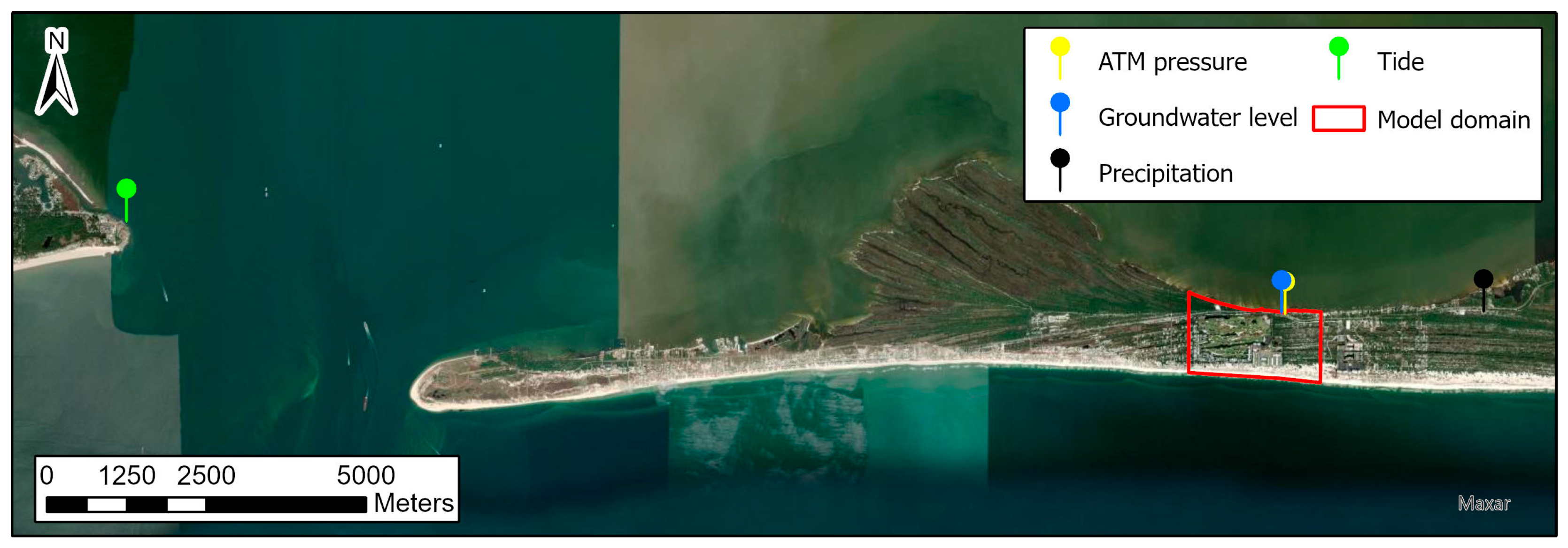
Several datasets were used to configure the GSSHA models, including the following: soil data from the Soil Survey Geographic (SSURGO) database for Baldwin County [33]; land cover data from the National Land Cover Database (NLCD); imagery from the National Agriculture Imagery Program (NAIP) [34], used to improve the resolution of the land cover classification using GeOBIA for the small-scale simulation [35]; and elevation data: based on our analysis, we utilized the one-meter Digital Elevation Model (DEM) from the U.S. Geological Survey (USGS) Coastal National Elevation Database (CoNED) Applications Project, as it is more recent and aligns with field investigations. Rainfall and tide data were also collected from the South Alabama Mesonet [31] and from NOAA Tides and Currents’ Dauphin Island station [36]. The Alabama Department of Transportation (DOT) supported the installation of one HOBO level logger, model U20L, to capture shallow groundwater elevation (Figure 2, red pin). In addition, the authors installed another level logger of the same model to measure atmospheric pressure close to the groundwater well (Figure 2, yellow pin).

2.3. Land Cover Classification Using GeOBIA

This study employed Geographic Object-Based Image Analysis (GeOBIA) on NAIP imagery to improve land cover classification. The eCognition Developer v10.1 software was used, with Band 1 designated as the red band, Band 2 as the green band, Band 3 as the blue band, and the last as the near-infrared band (NIR). Then, segmentation was processed using the Spectral Difference Segmentation algorithm, which identified the following classes: barren land, trees (forest), grass, shrub/scrub, buildings, paved areas, and water. Height classification was executed to enhance classification accuracy based on specific thresholds: buildings and trees exceeding 2 m (approximately 6 feet) in height, shrub/scrub ranging from 1 to 2 m (approximately 3 to 6 feet), and grass measuring less than 1 m (approximately 3 feet) in height [37,38]. This improved the identification of surface characteristics, yielding more realistic infiltration estimates and Manning’s roughness values (Figure 3).

2.4. Modeling

GSSHA modeling of the Boat Launch site was created with high spatial accuracy (i.e., 3 m calculation cells) aimed to represent infiltration, groundwater (GW) level fluctuation and saturation in a coastal setting. Key model configurations included the following:

• The Green–Ampt infiltration method was used, adjusting hydraulic conductivity to reflect local land cover. Paved surfaces were assigned lower infiltration rates to replicate urban runoff behavior. Infiltration was modeled using the Green–Ampt equation with redistribution, a method recognized as a close approximation to the numerical solution of Richards’ Equation [39].

  Table 1. Soil parameters based on estimates of [41] and [40].

  Land Cover	Manning’s n	Hydraulic Conductivity (cm/h)
  Trees	0.12	15
  Water	0.025	0.001
  Paved	0.016	1.5
  Shrub	0.1	15
  Barren Land	0.025	15
  Buildings	0.15	1.5
  Grass	0.035	1.5

  illustrates the remaining infiltration parameters used in this study. Hydraulic conductivities were reduced following the indices found by [40] for the different land cover classes.
• Surface roughness parameters were assigned based on the resultant land cover classifications shown in Figure 3. The authors converted the land use classification to a 3 m cell resolution raster, to improve software performance. Then, it was uploaded to the project and converted into a land use grid, which allowed Manning’s n values to be set for each land cover classification.
• Groundwater–surface water interactions were also included, accounting for additional parameters such as aquifer depth, initial water table elevations, hydraulic conductivity, and soil porosity.
• Initial water table elevation is spatially variable, with the levels matching Mobile Bay and the Gulf of America to the north and south boundaries, respectively. Higher water table elevations are assumed with increased distance from the coast, reaching 1 m above the current sea level at the start of the simulation. Furthermore, due to the same land use and elevation, GW flows are assumed not to occur through the east and west borders of the subcatchment. As a result, GW discharges occur only through the northern and southern borders of the model.

2.4.1. Model Setup

GSSHA enables the dynamic simulation of hydrologic processes, including precipitation, overland flow, infiltration, and groundwater flow, which are modeled in this study. First, overland flow is solved using the 2D diffusive wave approximation of the shallow water equations [39]. The fluxes in the x and y directions are denoted as p (Equation (1)) and q (Equation (2)), respectively. The depth is updated as follows, in Equation (3), which allows for lateral water movement between cells.

$$p_{i,j}^n={\displaystyle \frac{1}{n}}{\left(d_{i,j}^n\right)}^{5/3}{\left(S_{fx}\right)}^{1/2}$$

(1)

$$q_{i,j}^n={\displaystyle \frac{1}{n}}{\left(d_{i,j}^n\right)}^{5/3}{\left(S_{fy}\right)}^{1/2}$$

(2)

$$d_{i,j}^{n+1}=d_{i,j}^n+{\displaystyle \frac{∆t}{∆x}}\left(p_{i-1,j}^n+q_{i,j-1}^n-p_{i,j}^n-q_{i,j}^n\right)$$

(3)

where $d_{i,j}$ = water depth in the grid cell (i, j); n = Manning’s roughness coefficient; ∆t = time step; S_fx and S_fy = slopes in the x and y directions; and ∆x = cell size. Second, infiltration is calculated using the Green–Ampt method for each grid cell, as shown in Equations (4) and (5). This permits spatial variation in infiltration due to differences in soil type and land cover.

$$f_p=K_s\left(1+{\displaystyle \frac{{\phi }_f{\theta }_d}{F}}\right)$$

(4)

$$F_{t+∆t}=K_s∆t+F_t+{\phi }_f{\theta }_d\mathit{ln}\left({\displaystyle \frac{F_{t+∆t}+{\phi }_f{\theta }_d}{F_t+{\phi }_f{\theta }_d}}\right)$$

(5)

where f_p = infiltration rate; Ks = saturated hydraulic conductivity (referred to in this study as infiltration hydraulic conductivity (K_inf)); φ_f = capillary suction at the wetting front; θ_d = moisture deficit; and F = cumulative infiltration [42]. Lastly, groundwater flow simulation uses an adapted version of the two-dimensional free surface groundwater problem [43], but diagonal terms are ignored and transmissivity is assumed to be the product of saturated hydraulic conductivity and saturated depth (saturated surface to aquifer bottom) [39]. Equation (6) illustrates the calculation of groundwater flow.

$${\displaystyle \frac{\partial }{\partial x}}\left(K_{xx}B{\displaystyle \frac{\partial E_{ws}}{\partial x}}\right)+{\displaystyle \frac{\partial }{\partial y}}\left(K_{yy}B{\displaystyle \frac{\partial E_{ws}}{\partial y}}\right)=S{\displaystyle \frac{\partial E_{ws}}{\partial t}}+W_s\left(x,y,t\right)$$

(6)

where E_ws = groundwater table elevation, which is referred to in this study as groundwater level (GWL); K_xx and K_yy = saturated hydraulic conductivities on the x and y directions, referred to in the next sections as groundwater hydraulic conductivity (K_GW); B = depth of saturated soil, which is related to the aquifer bottom depth (Aq. Bot.); S = specific yield; and Ws = fluxes from infiltration and stream, if present.

The starting hydraulic conductivity of 17 cm/h was extracted from NRCS soil data [33]. The porosity for this study area was calculated in three different locations by [44], with the best approximation being 25%, which was then used in all the simulations. For groundwater boundary conditions, the average tidal water level for the simulated periods was 0.25 m, which was applied as a fixed boundary condition on the north and south boundaries of the model domain.

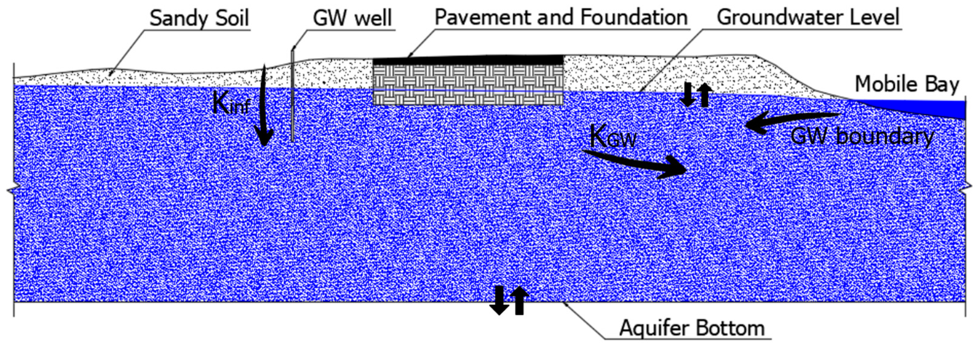
Three key structures were incorporated into the model: an embankment and two culverts, representing a double culvert at the model’s outlet. The embankment, located along AL-180 but constrained within the model domain, has a top elevation of 2.1 m and slopes of 0.13 toward the north and south. The culverts, each 0.61 m in diameter and 25 m in length, were placed at the intersection of the channel and the embankment. Overbank flow and backwater effects were removed from the channel setting to avoid instabilities, if the drainage area’s land cover and infiltration characteristics prevent significant overbank flow conveyance. Figure 4 illustrates the remaining parameters used for model calibration, which will be presented in the following sections.

2.4.2. Boundary Conditions

GSSHA does not allow tidal, time-varying water level boundary conditions for groundwater flow calculation. Such time-varying GW boundary conditions exist only for interactions between channels and shallow groundwater, as well as water withdrawal from wells. Therefore, the north and south boundaries were assumed to have a fixed groundwater level above the NAVD88 vertical datum, corresponding to the tide elevation at the start of the simulation. This is consistent with the stable water level methodology presented by [44], where the distance from the tidal body determines the water table elevation. Surface water level boundary conditions, on the other hand, can be represented as a fixed or variable level condition.

2.4.3. Model Evaluation

To evaluate the performance of the GSSHA model in representing observed groundwater levels, four statistical metrics were used: the Nash–Sutcliffe Efficiency (NSE), Root Mean Square Error (RMSE), Percent Bias (PBIAS), and the coefficient of determination (R²). NSE assesses the predictive power of the model by comparing the variance of the simulation error to the variance of the observed data; values closer to 1 indicate better agreement [45]. RMSE quantifies the average magnitude of the prediction error in the same units as the observed variable, where lower values represent more accurate predictions [46]. PBIAS measures the tendency of the simulated values to be larger or smaller than their observed counterparts, with values near zero indicating unbiased performance [47]. Finally, R² evaluates the strength of the linear relationship between observed and simulated values, reflecting how well the variation in observations is explained by the model [48].

3. Results

3.1. Calibration Results

The calibration began by adjusting GSSHA’s initial soil moisture parameter, which was initially set at 0.07 (7%). Groundwater saturated soil hydraulic conductivity (K_GW) and infiltration K values (K_inf) were tested between 15 cm/h and 45 cm/h, based on the ranges offered by [41]. However, K_inf was scaled according to the respective land cover, following the methodology presented by [40]. These changes primarily affected the groundwater baseline, but failed to reflect tidal dynamics, which are only enforced at the surface.

The model calibration was finalized by adjusting the physical parameters. The configuration with the best performance was the one with the aquifer bottom set at −12 m and infiltration and groundwater conductivities of 15 cm/h and 20 cm/h, respectively, accurately representing the observed peaks and recessions in the groundwater level (Figure 5f). This setup achieved a Nash–Sutcliffe Efficiency (NSE) of 0.9 and a Root Mean Square Error (RMSE) of 0.05 m for the calibration event. This occurred because increasing K_GW by more than 20 cm/h caused the model to respond too quickly to precipitation and recession, resulting in sharper recessions after precipitation stopped (Figure 5a,c). On the other hand, lowering K_GW and K_inf caused the model to overestimate GWLs (Figure 5d,e). In addition, increasing K_GW while maintaining the aquifer bottom at −12 m (Figure 5b,c) resulted in a more rapid recession, which deviated from observed data. Lowering the aquifer bottom without adjusting K_GW and K_inf may artificially elevate groundwater levels by increasing initial storage (Figure 5d,e).

Figure 5b,f presented better agreement with the observed peaks and recession trends, but the configuration in Figure 5f had a better NSE. Furthermore, a “warm-up” period was implemented before the first precipitation event to ensure realistic initial conditions for the validation scenarios, allowing the initial soil moisture in the model to stabilize. The final parameter values used in this study are shown in Table 1.

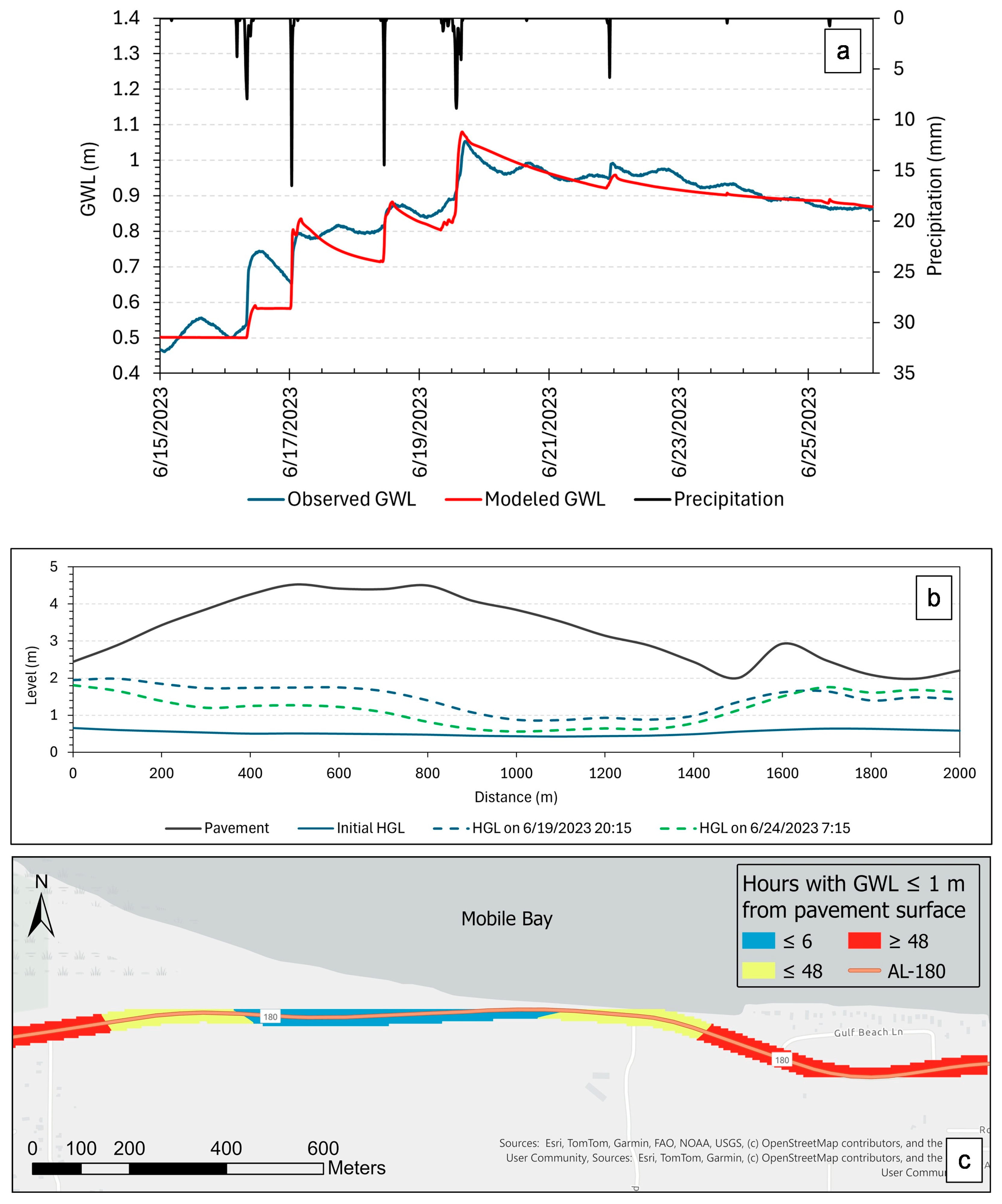
In addition to the temporal calibration (Figure 6a), the model was used to evaluate the spatial distribution of pavement saturation. Figure 6b,c display the results of this analysis, mapping the saturation along the 2 km stretch of AL-180. Figure 6b shows the most critical Hydraulic Grade Lines (HGLs) at two points in time during the simulation. In Figure 6c, saturation is defined as periods when the groundwater table is 1 m or less from the pavement surface. This spatial analysis identifies the highway segments that are most vulnerable to long-duration saturation, which poses a greater risk to pavement integrity, especially where the segments are located at lower elevations.

3.2. Validation Results

Two other field-observed datasets were used to validate the GSSHA model. A 14-day period (8–22 April 2023) and a 5-day period (3–8 September 2024) were simulated, including rainfall events that totaled 135 mm and 74 mm, respectively. In the first case (Figure 7a), the model closely follows the observed GWL, including the start of the groundwater rise of 13 April, but overestimates the magnitude of the peak GWL. In addition, the tidal sign shown in the observed time series is smoothed in the modeled GWL, as its influence on the variation of shallow groundwater cannot be represented. However, following the precipitation event, the model successfully represents the recession trend, with a slight overestimation (approximately 0.1 m) after 16 April.

Figure 7b shows the HGL along this section of AL-180. Interestingly, there were two moments of concern: the first represented the highest average peak GWL on 13 April, immediately after the first rainfall event; the second happened on 17 April, following a small precipitation event. The GWL approaches the pavement (0.9 to 0.3 m) between 1400 and 2000 m, similar to what is shown in Figure 6c for the calibration run. This coincides with the location of the drainage channel and a depression zone visible in the elevation profile.

For the second validation event (Figure 8a), the model accurately captured the groundwater response to multiple events that occurred between 5 September and 7 September 2024, following a warm-up period. The model underpredicted the GWL rise until September 6 and overpredicted it after that date, as it began to rise gradually, due to subsequent precipitation events. However, the error in both periods is approximately 0.05 m. Figure 6b displays the GWL profile along the same segment of AL-180. In this instance, the GWL remains 1 to 1.5 m away from the pavement between 1400 and 2000 m. However, the exposure times at the 1 m threshold were reduced to less than 4 h.

Decreasing the magnitude of rainfall also resulted in lower groundwater levels. This demonstrates the model’s ability to reflect variations in rainfall intensity and antecedent conditions across events. The saturation exposure is evident on the eastern side of this segment, indicating that it is the most sensitive section, where saturation occurs even for small rainfall events. However, prolonged high water table conditions only occurred for the calibration and first validation event, indicating a precipitation threshold that impacts the pavement. Also, when comparing the calibration and the first validation run, which have almost the same precipitation volume, the results suggest that pavement exposure is influenced not only by total rainfall, but also by rainfall distribution over time.

3.3. Model Performance

The calibration results showed strong agreement between observed and modeled groundwater levels, with an NSE of 0.900 and an R² of 0.934 (

Table 2. Model performance metrics.

	NSE	RMSE	PBIAS	R2
Calibration	0.900	0.069	2.274	0.934
Validation 1	0.842	0.118	−5.150	0.915
Validation 2	0.577	0.050	−0.010	0.833

), indicating that the model successfully captured both the magnitude and variability of the observed data. The RMSE of 0.069 m indicates a low average error, while the PBIAS of 2.27% suggests a slight model overestimation. Validation 1 also demonstrated good agreement between the observed and modeled GWL, with an NSE of 0.842 and an R² of 0.915. Although the RMSE increased to 0.118 m compared to calibration, this is expected, due to the different temporal characteristics of the validation event. The negative PBIAS value (−5.15%) indicates an underestimation of the groundwater levels, as shown in Figure 7a, and may be related to the lack of representation of tidal variations in the GWL, mostly before the rainfall event. The NSE for Validation 2 was 0.58, and the R² was 0.83, indicating acceptable ranges, although this suggests reduced predictive accuracy for this specific event. Interestingly, the RMSE was the lowest among the three cases (0.050 m), and the PBIAS was close to zero (−0.01%), indicating a low absolute error and minimal bias. The relatively low NSE may be attributed to the smaller amount of precipitation during this short 5-day simulation, which increases the relative error. This may result from the higher sensitivity of shallow groundwater levels to initial soil moisture conditions. Increasing the model resolution could help capture these small-scale variations, but would also substantially increase computational time.

3.4. Extreme Event Modeling

Figure 9 illustrates the spatial distribution of pavement surface saturation following Hurricane Sally in September 2020. The storm recorded a total precipitation of 555 mm and made landfall at Fort Morgan Peninsula before moving inland. Figure 7a depicts the rainfall/groundwater head relationship at our monitoring location. Figure 7b illustrates saturation along the entire segment during the most critical moments in terms of groundwater. Conversely, Figure 7c presents a detailed view of a 2 km segment of AL-180, focusing on the duration during which sections were saturated at a depth of less than 0.3 m from the pavement surface. Regarding pavement saturation, the results indicate an inland gradient, with longer saturation times observed as the road extends further from the coast. Over two-thirds of this section of the road remains saturated for more than 6 h, with a significant portion of the analyzed segment experiencing saturation for over 12 to 24 h, and in some areas exceeding 48 h, as illustrated by the red and orange segments. Finally, Figure 7c shows the variation in groundwater level (GWL) from the simulation’s start to the most critical GWL during the event along this road segment. According to the model results, the groundwater lens varied up to 4 m, depending on the location, reaching pavement surface level.

Some areas near the pavement also showed signs of flooding, mainly where the road shifted farther from Mobile Bay, similar to where prolonged saturation occurred (Figure 10a). According to the model results, flooding can vary from 0.3 to 1.0 m near the pavement in these two areas. In addition to the flooding, the groundwater level (GWL) took a long time to recede after the event. Therefore, the GWL may remain close to the pavement for extended periods, as observed between September 15th and 18th in Figure 10b. In the 100 m section, the GWL reaches the surface, which may lead to flooding and pressure from below. Conversely, the 1800 m section shows near-pavement saturation without flooding from below, and the surface flooding depicted in the figure is adjacent to the pavement.

4. Discussion

Hydrologic modeling in coastal environments presents unique challenges, due to interactions between precipitation, infiltration, and tidal variations. While the GSSHA model provides robust capabilities for simulating surface and shallow groundwater processes, its performance has proven variable, depending on the model configuration. Studies have indicated difficulty in calibrating GSSHA for sandy soils or in situations with limited hydrologic data. Because of its 2D formulation, GSSHA may better replicate groundwater dynamics than SWMM; however, replicating hydrographs remains challenging when groundwater contributions are dominant [29]. Additionally, their study lacked external forcing such as tidal variation. Other research has demonstrated that GSSHA model calibration can be effective, but is highly sensitive to parameters, including roughness, storage depth, and rainfall depth distribution [24,49].

Compared to commonly applied hydrologic models, such as SWMM and HEC-HMS, GSSHA offers advantages in simulating high-resolution shallow groundwater behavior. SWMM represents groundwater as a simplified linear reservoir for each subcatchment and lacks lateral groundwater flow, which may lead to unrealistic saturation distributions [29]. Similarly, HEC-HMS focuses on runoff processes, and was not designed to simulate groundwater fluctuations or surface water–groundwater interactions [27]. GSSHA, on the other hand, integrates 2D overland flow with 2D groundwater simulation on a gridded domain, to provide a more physically based approach [24,28]. However, a key limitation remains the model’s current inability to simulate time-varying tidal boundary conditions for groundwater, which restricts its application to compound flooding scenarios involving both storm surge and precipitation [30,50,51]. Nonetheless, the application presented in this study demonstrates that when carefully calibrated, GSSHA provides a robust platform for investigating water table-induced pavement vulnerability in low-lying coastal corridors.

In earlier studies at AL-180, simulations used synthetic storms and assumed a dry initial moisture condition [52]. Despite the high rainfall volumes (152–228 mm in 24 h), significant infiltration occurred, with limited overland flow and no flooding in some areas where flooding had previously been observed. This may be attributed to the area’s sandy soils and the lack of groundwater representation in the model, which limits infiltration. In addition, our study illustrates how significantly the initial water table and groundwater boundary conditions may influence GWL model predictions and need to be calibrated, as much as other parameters.

In this study, the model shows a satisfactory agreement with the observed GWL in both validation periods, capturing the general sub-daily trends and magnitudes of the response to precipitation and subsequent recession. This confirms GSSHA’s capabilities to represent the responses to high-intensity rainfall. The lower NSE for our second validation suggests limitations in representing smaller rainfall events. The pavement saturation analysis revealed that less intense events do not pose a threat. In addition, a sequence of rainfall events in the calibration demonstrated that antecedent moisture is critical in determining how long the pavement remains saturated. Lower elevations, on the other hand, may define where the pavement is vulnerable during less intense precipitation events.

Tidal interactions with groundwater are also critical in coastal hydrological simulations, but are not easily applied. Our GSSHA model represented sea level as a fixed boundary along Mobile Bay and the Gulf of Mexico. This approach aligns with [30], which coupled GSSHA with coastal inundation models to simulate storm surge dynamics. However, similar to what was shown in our study, other authors recognize GSSHA’s limitation in terms of representing dynamic tidal boundaries linked to astronomical cycles or storm surges [50,51]. This constraint may limit the simulation of real compound events, including extreme storm surges combined with higher initial water tables and precipitation. GSSHA response is highly influenced by grid resolution and Green–Ampt parameters [48]. In their case, they also reduced cell size and increased stream network, which affected predictions up to 57%. In our case, on the other hand, the saturated hydraulic conductivities for both infiltration and groundwater flows were calibrated, in addition to the aquifer bottom, which greatly influenced the magnitude of the GWL values. To reduce the uncertainty associated with K_inf and K_GW, field investigations can be complemented by laboratory soil tests. In addition, machine learning methods trained on historical observations can also be applied to automatically refine calibration through iterative optimization [53,54].

The extreme event simulation indicated that the pavement in the study area may remain saturated for several days. Prolonged saturation may increase pavement susceptibility to rutting, shear deformation, and premature failure under loading [55,56]. Additionally, flooding in locations adjacent to the pavement may result from poor drainage, leading to shoulder erosion and moisture accumulation in the pavement’s structural layers. Therefore, making it available for traffic before the GWL drains after an event such as Hurricane Sally could compromise the pavement’s structural reliability. There may be a need to delay the reopening of this segment of AL-180 after extreme events. The short saturation duration as AL-180 approaches Mobile Bay may be related to faster drainage conditions, indicating that the segment closer to the bay may be more vulnerable to storm surges than to higher water tables.

These results suggest that surface runoff alone under-represents the risks posed by flooding and high water tables at AL-180. However, validation demonstrated that the GSSHA model, as presented here, is suitable for detecting high groundwater levels near roadways, especially after intense precipitation events. Simulations predicting future rainfall, storms, and sea level conditions, including groundwater dynamics, are crucial for assessing elevated water table-induced saturation, particularly for low-lying infrastructure. While this study captured the dynamics of GWL changes and surface flooding, it does not explicitly address the potential impact of storm surges on infiltration processes because tidal variation cannot be represented in the groundwater simulation in GSSHA. Therefore, storm surge effects should be included [44] in future studies to enhance coastal vulnerability assessments, as they can increase water table elevations. To enhance the representation of tidal dynamics in groundwater simulations, future work could involve coupling GSSHA with coastal hydrodynamic models that simulate storm surge processes, which can be utilized as boundary or initial conditions. Additionally, empirical corrections based on observed tidal gauge data can be applied during post-processing [44]. In addition, future studies can include the effects of the interaction between freshwater and saltwater by monitoring groundwater electrical conductivity and using it to calibrate model parameters such as saturated hydraulic conductivity.

5. Conclusions

This study utilized GSSHA hydrologic modeling to evaluate groundwater level dynamics along a vulnerable section of AL-180 in Fort Morgan Peninsula, Alabama. The results indicated that GSSHA, when accurately calibrated, can depict the interactions between precipitation and shallow groundwater in sandy, low-lying coastal environments. The model effectively captured the timing and magnitude of groundwater peaks during validation and revealed extended periods of saturation following extreme events, such as Hurricane Sally. These findings emphasize that surface runoff alone fails to adequately capture the full complexity of hydrologic risks for coastal roads.

By incorporating groundwater processes, the simulations identified critical segments of the road that may remain saturated for hours or days, potentially compromising the pavement’s structural integrity if it is open to traffic immediately after the event ends. These results suggest that transportation agencies should consider delaying the reopening of roads such as AL-180 until groundwater levels have receded, to prevent long-term damage. Additionally, locations closer to the bay may require special attention for storm surge vulnerability, while inland segments are more sensitive to groundwater-induced saturation.

The modeling framework is replicable for similar coastal corridors characterized by sandy soils, high water tables, and proximity to tidal bodies. Other DOTs can adopt this method to prioritize infrastructure investments and establish road closure thresholds by accessing basic elevation, land cover, rainfall, and tide data. The use of Nature and Nature-Based Features (NNBF) such as wetlands, marsh creation, and water-resistant materials, such as geosynthetics or permeable asphalt, may help mitigate moisture damage. In addition, monitoring infrastructure, including soil moisture and groundwater sensors, such as the ones used in this study, could support predictive modeling for other coastal infrastructures.

Although the modeling approach addressed significant challenges such as high infiltration rates and shallow aquifers, limitations persist in representing tidal fluctuations within the groundwater component. Future studies should investigate coupling GSSHA with models that enable dynamic tidal boundary conditions or integrating manual tide-based corrections.

References

1. Easterling, D.R.; Kunkel, K.E.; Arnold, J.R.; Knutson, T.R.; LeGrande, A.N.; Leung, L.R.; Vose, R.S.; Waliser, D.E.; Wehner, M. Precipitation Change in the United States. In: Climate Science Special Report: Fourth National Climate Assessment. Fourth Natl. Clim. Assess. 2017, I, 207–230. [Google Scholar] [CrossRef]
2. Sun, Q.; Zhang, X.; Zwiers, F.; Westra, S.; Alexander, L.V. A Global, Continental, and Regional Analysis of Changes in Extreme Precipitation. J. Clim. 2021, 34, 243–258. [Google Scholar] [CrossRef]
3. Sweet, W.V.; Kopp, R.E.; Weaver, C.P.; Obeysekera, J.; Horton, R.M.; Thieler, E.R.; Zervas, C. Global and Regional Sea Level Rise Scenarios for the United States; NOAA Technical Report NOS CO-OPS 083; 2017; pp. 1–56. Available online: https://repository.library.noaa.gov/view/noaa/18399 (accessed on 11 June 2025).
4. Knott, J.F.; Daniel, J.S.; Jacobs, J.M.; Kirshen, P. Adaptation Planning to Mitigate Coastal-Road Pavement Damage from Groundwater Rise Caused by Sea-Level Rise. Transp. Res. Rec. 2018, 2672, 11–22. [Google Scholar] [CrossRef]
5. Cox, A.H.; Loomis, G.W.; Amador, J.A. Preliminary Evidence That Rising Groundwater Tables Threaten Coastal Septic Systems. J. Sustain. Water Built Environ. 2019, 5, 04019007. [Google Scholar] [CrossRef]
6. Peña, F.; Obeysekera, J.; Jane, R.; Nardi, F.; Maran, C.; Cadogan, A.; de Groen, F.; Melesse, A. Investigating Compound Flooding in a Low Elevation Coastal Karst Environment Using Multivariate Statistical and 2D Hydrodynamic Modeling. Weather. Clim. Extrem. 2023, 39, 100534. [Google Scholar] [CrossRef]
7. Lee, S.; Yen, H.; Yeo, I.Y.; Moglen, G.E.; Rabenhorst, M.C.; McCarty, G.W. Use of Multiple Modules and Bayesian Model Averaging to Assess Structural Uncertainty of Catchment-Scale Wetland Modeling in a Coastal Plain Landscape. J. Hydrol. 2020, 582, 124544. [Google Scholar] [CrossRef]
8. Yuan, L.; Mikelonis, A.M.; Yan, E. Using SWMM for Emergency Response Planning: A Case Study Evaluating Biological Agent Transport under Various Rainfall Scenarios and Urban Surfaces. J. Hazard. Mater. 2023, 458, 131747. [Google Scholar] [CrossRef] [PubMed]
9. Palanisamy, B.; Borkar, R.; Sangeetha, K.; Narasimhan, B. Evaluation of Augmented Infiltration Based LIDs for Low Lying Urbanizing Coastal Catchments: A Case Study of Chennai City, India. Urban. Water J. 2024, 21, 638–655. [Google Scholar] [CrossRef]
10. Vasconcelos, J.G.; Fang, X.; Geller, V.G.; Nicolaico, G.G.; Reyes, E.M. Resilient Design with Distributed Rainfall-Runoff Modeling; Transportation Research Board: Washington, DC, USA, 2023; ISBN 978-0-309-69861-0. [Google Scholar]
11. Ahmari, H.; Hummel, M.; Chao, S.-H.; Md Imran Kabir, S.; Pervaiz, F.; Acharya, B.R.; Dean, M.; Mowla, Q.A.E. Identify and Analyze Inundated Bridge Superstructures in High Velocity Flood Events; United States Department of Transportation: Arlington, VA, USA, 2021.
12. Thomas, W.; Newell, D.; Bernzott, E.; Szekeres, D.; Harris, J.; Tabb, C.; Siddiquee, F. Development of Site-Specific Hydrologic and Hydraulic Analyses for Assessing Transportation Infrastructure Vulnerability & Risks to Climate Change; United States Department of Transportation: Harrisburg, PA, USA, 2020.
13. Giacomoni, M.H.; Olivera, F.; do Lago, C. Assessing the Impacts of Super Storm Flooding in the Transportation Infrastructure–Case Study: San Antonio, Texas; United States Department of Transportation: Baton Rouge, LA, USA, 2019.
14. Vasconcelos, J.G.; Fang, X.; Anderson, J.B.; Tamang, S.; Song, W. Analysis and Potential Solutions to Sediment Deposition in Dean Road Bridge Watershed, Midland City, AL; United States Department of Transportation: Auburn, AL, USA, 2018.
15. Schwartz, J.S. Evaluation and Prediction of Bridge Pier and Contraction Scour of Cohesive River Sediments in Tennessee; United States Department of Transportation: Knoxville, TN, USA, 2018.
16. Zhang, Q.; Lu, Q.; Kwon, C.; Xu, X.; Schreiber, D. Spatial Sustainability Assessment of Green Stormwater Infrastructure for Surface Transportation Planning, Phase I; University of South Florida, Center for Transportation, Environment, and Community Health, U.S. Department of Transportation: Tampa, FL, USA, 2018. [Google Scholar]
17. Herb, W.; Janke, B.; Stefan, H. Study of De-Icing Salt Accumulation and Transport Through a Watershed; Minnesota Department of Transportation, Research Services & Library: Minneapolis, MN, USA, 2017. [Google Scholar]
18. Hoogestraat, G. Rainfall-Runoff Modeling for Improved Peak Flow Estimates in the Black Hills Area of South Dakota; United States Department of Transportation: Rapid City, SD, USA, 2017. [Google Scholar]
19. Scharffenberg, W. Hydrologic Modeling System HEC-HMS User’s Manual; Hydrologic Engineering Center (HEC), U.S. Army Corps of Engineers: Davis, CA, USA, 2016.
20. Rossman, L.A. Storm Water Management Model User’s Manual Version 5.1; United States Environmental Protection Agency (U.S. EPA), National Risk Management Research Laboratory (NRMRL), Office of Research and Development (ORD): Cincinnati, OH, USA, 2015.
21. Bragg, M.A.; Poudel, A.; Vasconcelos, J.G. Comparing SWMM and HEC-RAS Hydrological Modeling Performance in Semi-Urbanized Watershed. Water 2025, 17, 1331. [Google Scholar] [CrossRef]
22. Kampf, S.K.; Burges, S.J. A Framework for Classifying and Comparing Distributed Hillslope and Catchment Hydrologic Models. Water Resour. Res. 2007, 43, 5370. [Google Scholar] [CrossRef]
23. Downer, C.W.; Ogden, F.L. Prediction of Runoff and Soil Moistures at the Watershed Scale: Effects of Model Complexity and Parameter Assignment. Water Resour. Res. 2003, 39, 1439. [Google Scholar] [CrossRef]
24. Weston, D.M.; Skahill, B.E.; Downer, C.W.; Graulau-Santiago, J.A.; Pradhan, N.; Byrd, A.R. Gridded Surface Subsurface Hydrologic Analysis Modeling for Analysis of Flood Design Features at the Picayune Strand Restoration Project. In Proceedings of the World Environmental and Water Resources Congress 2015, Austin, TX, USA, 17–21 May 2015; pp. 1500–1511. [Google Scholar] [CrossRef]
25. Brendel, C.E.; Dymond, R.L.; Aguilar, M.F. Modeling Storm Sewer Networks and Urban Flooding in Roanoke, Virginia, with SWMM and GSSHA. J. Hydrol. Eng. 2021, 26, 5020044. [Google Scholar] [CrossRef]
26. Fry, T.J.; Maxwell, R.M. Using a Distributed Hydrologic Model to Improve the Green Infrastructure Parameterization Used in a Lumped Model. Water 2018, 10, 1756. [Google Scholar] [CrossRef]
27. Hamedi, A.; Fuentes, H.R. Comparative Effectiveness and Reliability of NEXRAD Data to Predict Outlet Hydrographs Using the GSSHA and HEC-HMS Hydrologic Models. 2015, pp. 1444–1453. Available online: https://ascelibrary.org/doi/10.1061/9780784479162.142 (accessed on 11 January 2024).
28. Sith, R.; Nadaoka, K. Comparison of SWAT and GSSHA for High Time Resolution Prediction of Stream Flow and Sediment Concentration in a Small Agricultural Watershed. Hydrology 2017, 4, 27. [Google Scholar] [CrossRef]
29. Moore, M.F.; Vasconcelos, J.G.; Zech, W.C. Modeling Highway Stormwater Runoff and Groundwater Table Variations with SWMM and GSSHA. J. Hydrol. Eng. 2017, 22, 1–15. [Google Scholar] [CrossRef]
30. Karamouz, M.; Ahmadvand, F.; Zahmatkesh, Z. Distributed Hydrologic Modeling of Coastal Flood Inundation and Damage: Nonstationary Approach. J. Irrig. Drain. Eng. 2017, 143, 1–14. [Google Scholar] [CrossRef]
31. Kimball, S.K.; Terwey, W. South Alabama Mesonet. Available online: http://chiliweb.southalabama.edu/archived_data.php (accessed on 21 September 2024).
32. Beck, H.E.; Zimmermann, N.E.; Mcvicar, T.R.; Vergopolan, N.; Berg, A.; Wood, E.F. Data Descriptor: Present and Future Köppen-Geiger Climate Classi Fi Cation Maps at 1 -Km Resolution. Sci. Data 2018, 5, 1–12. [Google Scholar] [CrossRef] [PubMed]
33. Soil Survey Staff Web Soil Survey. Available online: http://websoilsurvey.sc.egov.usda.gov/ (accessed on 11 January 2024).
34. OCM Partners AIP Digital Orthophoto (DOQQ—Quarter-Quadrangle) M_3008749_nw_16_030_20211113 2022. (2022). Available online: https://www.fisheries.noaa.gov/inport/item/49502 (accessed on 1 August 2025).
35. Dewitz, J. National Land Cover Database (NLCD) 2019 Products (Ver. 3.0, February 2024). (2024). Available online: https://doi.org/10.5066/P9KZCM54 (accessed on 27 April 2025).
36. NOAA NOAA Dauphin Island, AL—Station Home Page. Available online: https://tidesandcurrents.noaa.gov/stationhome.html?id=8735180&units=metric (accessed on 2 July 2024).
37. Gilman, E.F. Spartina Bakeri Marsh Grass, Sand Cordgrass; EDIS: Gainesville, FL, USA, 2023. [Google Scholar]
38. UC Santa Barbara Coastal Sage Scrub. Available online: https://www.ncos.ccber.ucsb.edu/native-plant-habitats/coastal-sage-scrub (accessed on 9 March 2023).
39. Downer, C.W.; Ogden, F.L. Gridded Surface Subsurface Hydrologic Analysis (GSSHA) User’s Manual, Version 1.43 for Watershed Modeling System 6.1; US Army Corps of Engineers, Engineer Research and Development Center: Vicksburg, MS, USA, 2006. [Google Scholar]
40. Robinson, D.A.; Nemes, A.; Reinsch, S.; Radbourne, A.; Bentley, L.; Keith, A.M. Global Meta-Analysis of Soil Hydraulic Properties on the Same Soils with Differing Land Use. Sci. Total Environ. 2022, 852, 158506. [Google Scholar] [CrossRef] [PubMed]
41. Rawls, W.J.; Brakensiek, D.L.; Saxton, K.E. Estimation of Soil Water Properties. Trans. ASAE 1984, 25, 1316–1320. [Google Scholar] [CrossRef]
42. Mein, R.G.; Larson, C.L. Modeling Infiltration during a Steady Rain. Water Resour. Res. 1973, 9, 384–394. [Google Scholar] [CrossRef]
43. Trescott, P.C.; Pinder, G.F.; Larson, S.P. Finite Difference Model for Aquifer Simulation in Two Dimensions with Results of Numerical Experiments; U.S. Geological Survey (USGS) Water Resources Division: Arlington, VA, USA, 1976.
44. De Oliveira Sousa, B.J.; Webb, B.M.; Wright, D.B.; Clement, T.P.; Vasconcelos, J.G. Conceptual Data-Driven Approach for Analyzing the Vulnerability of Coastal Roadways to Groundwater Level Changes. J. Environ. Manag. 2025, 390, 126295. [Google Scholar] [CrossRef] [PubMed]
45. Nash, J.E.; Sutcliffe, J.V. River Flow Forecasting through Conceptual Models Part I—A Discussion of Principles. J. Hydrol. 1970, 10, 282–290. [Google Scholar] [CrossRef]
46. Willmott, C.J. Some Comments on the Evaluation of Model Performance. Bull. Am. Meteorol. Soc. 1982, 63, 1309–1313. [Google Scholar] [CrossRef]
47. Gupta, H.V.; Sorooshian, S.; Yapo, P.O. Status of Automatic Calibration for Hydrologic Models: Comparison with Multilevel Expert Calibration. J. Hydrol. Eng. 1999, 4, 135–143. [Google Scholar] [CrossRef]
48. Legates, D.R.; McCabe, G.J. Evaluating the Use of “Goodness-of-fit” Measures in Hydrologic and Hydroclimatic Model Validation. Water Resour. Res. 1999, 35, 233–241. [Google Scholar] [CrossRef]
49. Chintalapudi, S.; Sharif, H.; Xie, H. Sensitivity of Distributed Hydrologic Simulations to Ground and Satellite Based Rainfall Products. Water 2014, 6, 1221–1245. [Google Scholar] [CrossRef]
50. Fattahi, A.M.; Hosseini, K.; Farzin, S.; Mousavi, S.-F. An Innovative Approach of GSSHA Model in Flood Analysis of Large Watersheds Based on Accuracy of DEM, Size of Grids, and Stream Density. Appl. Water Sci. 2023, 13, 33. [Google Scholar] [CrossRef]
51. Wijayarathne, D.B.; Gomezdelcampo, E. Using Shallow Groundwater Modeling to Frame the Restoration of a Wet Prairie in the Oak Openings Region, Ohio, USA: GSSHA Model Implementation. Environ. Earth Sci. 2019, 78, 216. [Google Scholar] [CrossRef]
52. Sousa, B.J.O.; Vasconcelos, J.G. GSSHA Modeling Applied to a Coastal Roadway in Alabama. In Proceedings of the World Environmental and Water Resources Congress 2024; American Society of Civil Engineers: Milwaukee, WI, USA, 2024; pp. 716–723. [Google Scholar]
53. Wang, C.; Jiang, S.; Zheng, Y.; Han, F.; Kumar, R.; Rakovec, O.; Li, S. Distributed Hydrological Modeling With Physics-Encoded Deep Learning: A General Framework and Its Application in the Amazon. Water Resour. Res. 2024, 60, e2023WR036170. [Google Scholar] [CrossRef]
54. Tukeev, D.L.; Afanaseva, O.V.; Tulyakov, T.F. Realization of Statistical Models Based on Symmetric Unimodal Distributions. Int. J. Eng. 2026, 39, 407–419. [Google Scholar] [CrossRef]
55. Chen, X.; Wang, H. Impact of Sea Level Rise on Asphalt Pavement Responses Considering Seasonal Groundwater and Moisture Gradient in Subgrade. Transp. Geotech. 2023, 40, 100992. [Google Scholar] [CrossRef]
56. Titus-Glover, L.; Darter, M.I.; Von Quintus, H. Impact of Environmental Factors on Pavement Performance in the Absence of Heavy Loads; U.S. Department of Transportation (USDOT) Federal Highway Administration (FHWA): McLean, VA, USA, 2019.
Figure 1. Study area. The water body to the north is Mobile Bay, and the one to the south is the Gulf of America. The red circle corresponds to the location of Fort Morgan Peninsula in the state of Alabama.
Water 17 02327 g001
Figure 2. Monitoring locations.
Water 17 02327 g002
Figure 3. Comparison between National Landcover Database (NLCD) data (a) and Geographic Object Based Image Analysis (GeOBIA) (b) land use classifications.
Water 17 02327 g003
Figure 4. Diagram of the parameters used for calibration, including the aquifer bottom level, infiltration hydraulic conductivity (Kinf), and groundwater hydraulic conductivity (KGW). The up and down arrows represent both the groundwater level variation and the changes in the aquifer bottom elevation.
Water 17 02327 g004
Figure 5. Exploratory variation in groundwater saturated soil hydraulic conductivity (KGW), surface infiltration K values (Kinf), and the elevation of the aquifer bottom. (a) first calibration trial; (b) second calibration trial; (c) third calibration trial; (d) fourth calibration trial; (e) fifth calibration trial; (f) final calibration trial.
Water 17 02327 g005
Figure 6. Calibration results for a 10-day event. This simulation yielded an RMSE of 0.9. (a) GWL time series at the location where the monitoring was performed; (b) groundwater level along AL-180 during peak times; (c) saturation along this 2 km section of AL-180.
Water 17 02327 g006
Figure 7. Validation results for a 14-day event. This simulation yielded an RMSE of 0.9. (a) GWL time series at the location where the monitoring was performed; (b) groundwater level along AL-180 during peak times; (c) saturation along this 2 km section of AL-180 at a 1 m threshold.
Water 17 02327 g007
Figure 8. Validation results for a 5-day event. This simulation yielded an RMSE of 0.58. (a) GWL time series at the location where the monitoring was performed; (b) groundwater level along AL-180 during peak times; (c) saturation along this 2 km section of AL-180 at a 1 m threshold.
Water 17 02327 g008
Figure 9. GWL results from the simulation of the same area for Hurricane Sally, which happened in September 2020, with 555 mm of rainfall. (a) Rainfall/groundwater head relationship at our monitoring location; (b) saturation along the whole segment; (c) detailed view of the segment with the duration during which sections were saturated at less than 0.3 m from the pavement surface.
Water 17 02327 g009
Figure 10. Flooding and GWL results from the simulation of the same area for Hurricane Sally, which happened in September 2020, with 555 mm of rainfall. (a) flooding depth along this section of AL-180 at peak flood time; (b) Groundwater level variation along the simulation time for the solid (at 200 m) and the dashed (at 1700 m) ellipses marked in (a).
Water 17 02327 g010