Abstract
Climate change is projected to significantly alter hydrological conditions across the Northern Hemisphere, with increased precipitation variability, more intense rainfall events, and earlier, rain-driven spring floods in regions like northern Sweden. These changes will affect both natural ecosystems and hydropower-regulated rivers, particularly during ecologically sensitive periods such as the grayling spawning season in late spring. This study examines the impact of extreme spring flow conditions on grayling spawning habitats by analyzing historical runoff data and simulating high-flow events using a 2D hydraulic model in Delft3D FM. Results show that previously suitable spawning areas became too deep or experienced flow velocities beyond ecological thresholds, rendering them unsuitable. These hydrodynamic shifts could have cascading effects on aquatic vegetation and food availability, ultimately threatening the survival and reproductive success of grayling populations. The findings underscore the importance of integrating ecological considerations into future water management and hydropower operation strategies in the face of climate-driven flow variability.
1. Introduction
Future climate projections for the Northern Hemisphere indicate a warmer climate with increased variability in hydrological conditions [1,2]. It is expected that precipitation patterns will become more erratic, with an increase in total precipitation, higher variability in rainfall, and a greater likelihood of both intense rainfall events over short periods and extended drought periods [3].
In northern Europe and North America, climate models predict warmer summers, which will increase the risk of drought [4], while winters will become wetter, with more precipitation falling as rain rather than snow [5]. This shift will lead to a reduced duration of ice cover, and the spring floods in northern Sweden will be more rain-driven and up to one month earlier [6]. Climate change is anticipated to have profound impacts on ecosystems within flowing watercourses, primarily through alterations in temperature and water flow [1]. These changes will stem from shifting precipitation patterns, which will influence the hydrological cycle [7]. As a result, ecosystems will experience direct effects from these changes, but there will also be significant indirect consequences that affect food availability, predator-prey dynamics, and overall ecosystem health [8].
To gain a realistic understanding of how these extreme flow conditions might affect the grayling (Thymalus thymallus) spawning habitat, this project has initiated an analysis based on historical data. Grayling was selected as the focal species for this study because it is native to the area, its distribution in the region is well-documented, and it exhibits narrow ecological preferences, making it a suitable indicator species for assessing environmental change. Over the past 30 years, runoff and discharge data have been compared, revealing several instances where runoff levels were exceptionally high, coinciding with similarly elevated discharge levels through the hydropower plants. One of these extreme flow events has been simulated using a 2D hydrodynamic model in Delft 3D FM, which incorporates real-flow data from the hydropower plants’ discharge and spill schedules on a 24 h mean basis.
In addition to the direct biological impacts, climate change will influence the operation of hydropower systems [9]. As climate change leads to more erratic weather patterns, the operation of hydropower plants will likely become more challenging [10]. Increased variability in flow, particularly in waterways developed for hydropower, will result in greater fluctuations, with extreme variations from zero flow to high flow over relatively short periods. Such extremes will likely put additional pressure on the management and sustainability of hydropower infrastructure and the ecological status of the river ecosystem [11]. The effects of climate change on hydropower and aquatic ecosystems are intertwined, making it essential to study how these changes will manifest over time. Understanding how water flow and temperature will fluctuate under future climate scenarios is crucial for predicting the potential impacts on aquatic life and for developing strategies to mitigate these effects. Without comprehensive studies on how climate change will alter the flow regimes in these waterways, it will be difficult to develop effective management strategies for both the ecosystems and the hydropower systems.
Grayling populations are dependent on temperature and flow variations and will be affected due to climate change and flow variations [12]. Special attention was given to the timing of this flow event, which occurred at the turn of May to June—an ecologically significant period for many aquatic species. During this critical window, grayling engage in spawning and early development. If flow conditions and temperature are altered due to climate change during this period, it has consequences for the survival and growth of these organisms [13].
Previous studies on extreme flow events have shown that unusually large spring floods can negatively impact the abundance of juvenile fish. Flood events led to a reduction in benthic invertebrate taxa in both channelized and natural river cross-sections [14]. Such extreme hydrological disturbances—including both floods and droughts—have been reported to reduce habitat availability and biodiversity [15]. By modeling a potential extreme flow event, it is possible to predict how future changes in the river could be affected.
Worldwide, the flood regimes of numerous river ecosystems have been substantially altered due to a disrupted hydrological cycle, influenced by heightened climate variability and human-induced pressures [16,17]. Warmer temperatures have led to more frequent snowmelt-induced floods during spring, particularly across northeastern Europe. Analyses of flood timing over the past 50 years have revealed clear temporal shifts that can be attributed to climate-related effects [17,18].
2. Materials and Methods
2.1. General Approach
The approach for this study has been to examine historical precipitation and historical flow data throughout the studied area. Since flow data from hydropower plants and runoff data are not always consistent due to the regulation of hydropower on the electrical grid, both types of data have been analyzed together to identify instances when they coincide. An interesting event was identified and studied in more detail.
By modeling the significant flow event in the hydraulic model, detailed information about how an extreme case manifests in hydraulic parameters such as water depth, flow velocity, and bed shear stress is obtained. These parameters have been analyzed in relation to known ecological preferences in order to assess how extreme events affect the ecosystem and the ability of grayling to reproduce in the studied area.
2.2. Study Site
This study focuses on an area between two hydropower plants in a heavily regulated river in northern Sweden. This section of the river is part of the Lilla Lule River and is located north of the Arctic Circle. The studied stretch is situated outside the town of Jokkmokk, in an area of interest for outdoor recreation. Here, the river alternates between more rapid-flowing segments and calmer stretches with pools.
This region has been the subject of previous research, primarily focusing on grayling habitat and the identification of suitable spawning areas [19]. Past studies have been conducted under normal flow conditions, examining how these conditions affect areas of interest [20]. However, research into extreme flow conditions and their potential ecological impacts has not been conducted before. There is limited knowledge about how the river is affected during very high flows. Given that such extreme events are expected to become more frequent in the future, it is crucial to investigate how these flows might impact the area and whether the operations of the two power plants could be leveraged to mitigate such effects.
The model focuses on a 15 km stretch of the river identified as having the highest potential for effective grayling habitat restoration [19].
The model is constructed using three different Digital Elevation Model (DEM) datasets, which are combined within the ArcGIS Pro 3.4.0 software. The DEM data was provided by Vattenfall AB, while land area and floodplain data were sourced from the Swedish Land Survey Authority (Lantmäteriet). The reference system used is SWEREF 99TM [19].
In previous studies, six pressure loggers were deployed to measure depth, and a Real-Time Kinematic (RTK) GPS pole was used to obtain elevation data for the pressure loggers [21]. By combining depth and elevation measurements, the water surface elevation (WSE) could be calculated. These data were then used to validate the model against recorded water flows from June to September 2021 [19]. Previous studies [19] have identified two areas in the river as the most suitable spawning habitats for grayling. Figure 1 illustrates the upstream and downstream spawning areas.
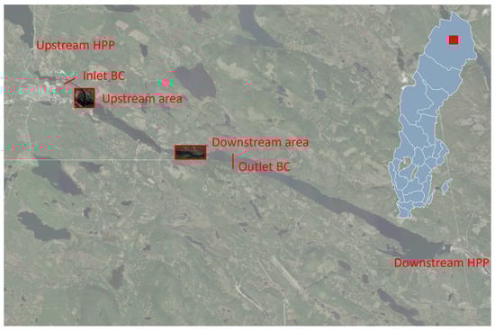
Figure 1.
Study reach with upstream and downstream areas studied in more detail. The location of the two hydropower plants (HPP) and the modeled stretch with inlet and outlet.
2.3. Hydrological Analysis
By studying historical flow data, interesting extreme events have been identified. On several occasions, the runoff in the area was high while the flow through the power plants was also elevated. However, since hydropower plants adjust their flow based on electricity production for the grid, high inflows do not always correlate with high flows through the power plant; see Figure 2. Therefore, studying the impact of climate change involves examining the future inflow trends and considering how hydropower is likely to be utilized in an electrical grid with renewable energy sources [22].

Figure 2.
(a) Historical discharge and runoff in the studied area from 1972 to 2015. (b) Discharge and runoff in 1995.
Figure 2 shows a historical discharge curve along with runoff data from the studied power plants. A closer examination reveals that high inflows and discharge coincided in 1995. Further analysis shows an event where water flow transitions from low to high flow within a short time period, as illustrated in Figure 2. The spring flood of 1995 was one of the largest of the century and occurred due to a snow-rich winter and simultaneous snowmelt in both forest and mountain areas, resulting in a combined forest and mountain flood. Heavy rainfall during the intense snowmelt period from 17 May to 9 June further contributed to the flood. In the regulated rivers, it was possible to store a large portion of the spring flood in the regulation reservoirs, and without these regulations, many of the watercourses would have experienced significantly higher flows [23]. To explore the potential ecological impacts of such extreme events, the model was run over approximately a month period during which the extreme flow event occurred. The resulting simulations provided valuable insight into the variations in water levels and velocities and their consequences for the local grayling spawning habitats.
A simulation was conducted from May to June, as the flows in April and May, shown in the discharge curve above (Figure 2), were very low and increased sharply to high levels over a few weeks. Due to the time-consuming nature of running the simulation, only the period of interest was simulated.
In the absence of data from the historical event, the downstream water level was varied based on analogous spring flood events, during which the lower dam is emptied in advance and then refilled over the course of a spring flood event. Figure 3 shows the discharge curve that was simulated, along with the downstream water surface elevation that was used as a boundary condition.
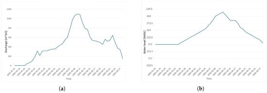
Figure 3.
Boundary conditions applied in the simulation model (a). Discharge used as inlet boundary condition (b). Water level as outlet boundary condition.
2.4. Numerical Modeling
The 2D hydraulic model was developed using Delft3D FM. It employs a finite volume solver to compute the depth-averaged velocities by solving the Navier-Stokes equations under the Boussinesq and shallow water assumptions [24]. The model’s time step is automatically calculated based on the Courant criterion, with a default Courant number of 0.7. The upstream boundary condition was defined using historical discharge data provided by SMHI [25]. The downstream boundary condition was defined as the water surface elevation.
A comprehensive mesh study for the hydraulic model has been performed in previous studies by [26]. The domain is discretized with a flexible mesh in the module RGFGRID in Delft 3D FM. The grid is built up by rectangular elements in the main channel and triangular elements in the areas peripheral to the main channel [26].
The roughness was calibrated in six parts of the domain adapted from [26], with the final roughness presented in Table 1.

Table 1.
Roughness coefficients for different areas [26].
2.5. Combining Fish Data and Hydraulics
Previous studies have identified the preferred parameters for grayling, and data from these studies have been used to analyze areas of interest in this study. A compilation of the grayling’s preferred flow conditions and substrate types is presented in Table 2 with data from [27,28,29,30]. This data has been used to assess how extreme flow events have affected the different stages of grayling.
Table 2.
Grayling preferences [27,28,29,30].
2.6. Scouring
One of the major consequences of elevated river flows is the scouring of redds (nests), which can significantly impact fish reproduction success rates [31]. Redd scouring occurs when the gravel or sand in which eggs are buried is displaced by the force of flowing water. This can lead to the exposure of eggs to drier zones or areas with suboptimal hydraulic conditions, ultimately increasing egg mortality [32,33].
The likelihood of redd scouring can be assessed using sediment transport theory. A key concept in this context is the Shields parameter, which predicts the initiation of sediment movement due to flow-induced forces. The threshold at which particles begin to move—known as the critical Shields stress—is defined as
Here, represents the dimensionless critical Shields stress, is the bed shear stress at the onset of particle motion, is the sediment density, is the water density, g is the acceleration due to gravity, and D is the particle diameter. This critical value varies with river flow conditions, but for gravel-bed rivers, it typically falls within the range of 0.03 to 0.06 [34,35,36].
When the actual bed shear stress exceeds the critical threshold, sediment particles begin to mobilize. If redds are located within these mobile sediments, the eggs may be dislodged and swept away, reducing egg-to-fry survival rates and ultimately threatening the long-term sustainability of fish populations in these habitats.
For European grayling, suitable spawning substrates generally include coarse gravel (8–16 mm), fine pebble (16–32 mm), and coarse pebble (32–64 mm), with an optimal grain size reported to be between 16 and 32 mm [37].
The critical shear stress was calculated by [26] to evaluate the risk of redd scouring in the river. Based on this approach, the threshold was divided into three categories, where the dimensionless critical Shields stress for gravel was estimated at 0.03 for easily mobilized particles and 0.045 for more stable substrates [36]. For European grayling, the spawning substrate was assumed to range from 16 to 64 mm in diameter [37]. The calculated critical shear stress values corresponding to the lower and upper bounds of this gravel size range are presented in Table 3 with the data adapted from [26].
Table 3.
Critical bed shear stress for spawning gravel sizes: fine (16–32 mm) and coarse (32–64 mm) pebbles [26].
3. Results
3.1. Flow Variation and Its Effect on Grayling Spawning Habitat
The critical flow events occur when the water level is at its lowest, with a low flow through the turbines, and when the water level is at its highest, with a high flow through the turbines. Therefore, these two flow scenarios have been visualized to enable a comparison of how the different flow conditions affect the developmental stages of grayling.
As shown in Figure 4, water velocities are close to zero during the low-flow period, which extends from April to the end of May, with occasional peaks indicating slightly increased flow. This sustained low flow included several zero-flow events. Based on the reference in Table 2, suitable spawning areas under low-flow conditions are illustrated in Figure 4. These areas are primarily concentrated in the center of the main channel at the outlet, where water velocities remain slightly higher. This does not take the bottom substrate into account but is only an estimate of suitable water depth and velocity from Table 2.

Figure 4.
(a) Velocity magnitude on 20th of May during low flow in the upstream area. (b) Suitable spawning habitats on 20th of May during low flow. Red dots are suitable spawning areas, green dots are points studied over time.
In mid-June, the flow is significantly higher, leading to increased water velocities as shown in Figure 5. This change in flow conditions can have serious implications for grayling eggs and fry that were produced during the earlier low-flow period. According to Table 2, larvae and fry prefer water velocities between 0.1 and 0.5 m/s, a range that is greatly exceeded during high-flow events. At such velocities, small larvae and fry likely struggle to maintain their position in the current, increasing the risk of being swept downstream into less suitable habitats.
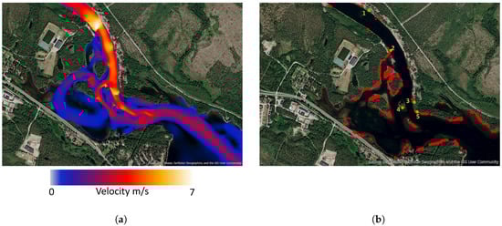
Figure 5.
(a) Velocity magnitude on 10th of June during high flow in the upstream area. (b) Suitable spawning habitats on 10th of June during high flow. Red dots are suitable spawning areas, green dots are points studied over time.
A considerably larger number of suitable spawning areas are present under high-flow conditions, as illustrated in Figure 5. However, it is also essential to examine how long an area remains suitable for spawning.
In the downstream area, no water velocities exceeded the minimum requirements for suitable habitats during the low-flow period, and consequently, no suitable spawning habitats were identified under those conditions. Figure 6 shows the water velocities during the high-flow event. Despite the same overall discharge, the velocities here are not as high as in the upstream section. Suitable spawning habitats, based on the criteria in Table 2, are shown in Figure 6.
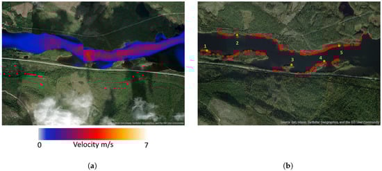
Figure 6.
(a) Velocity magnitude on 10th of June during high flow in the downstream area. (b) Suitable spawning habitats on 10th of June during high flow. Red dots are suitable spawning areas; green dots are points studied over time.
3.2. Bed Shear Stress and Potential Redds Scouring
Bed shear stress varies with discharge. Under low-flow conditions, bed shear stress approaches zero due to minimal water velocity. The upstream area is more affected, with larger zones reaching critical shear stress levels. In contrast, the downstream area exhibits fewer zones exposed to critical levels during high flows, as illustrated in Figure 7. Coarser substrate in these areas can enhance stability and provide shelter, helping fry and larvae remain in place despite elevated shear stress.

Figure 7.
(a) Bed shear stress during high flow in the upstream area (b). Bed shear stress during high flow in the downstream area.
3.3. Time Variation for Critical Habitat Limits
By studying potential spawning habitats over time, it is possible to assess both the duration and timing during which an area may be suitable for grayling. It is not only the quantity of suitable spawning habitats that is important to preserve, but also the length of time they remain viable. From Figure 4b, five observation points have been monitored over time, with Point 1 located furthest upstream and subsequent points positioned progressively downstream. These points were analyzed with respect to velocity, water depth, and bed shear stress, as shown in Figure 8. The spawning areas that were utilized when suitable are later exposed to critical flow velocities and depths, as illustrated in Figure 8. Several of the points remain below the critical threshold for bed shear stress (see Figure 8), indicating that redds and eggs are unlikely to be subjected to scouring.

Figure 8.
(a) Velocity for observation points at low flow in upstream area with critical limits for spawning habitats (b). Water depth for observation points at low flow in upstream area with critical limits for spawning area. (c) Bed shear stress with critical limits in colors, no risk, potential risk, and high risk, for gravel size of 16 mm.
Similarly, five points were analyzed within the identified spawning areas for high flow shown in Figure 5b. Flow velocities, water depths, and bed shear stress at these points are presented in Figure 9. Suitable water velocities are present during the period from June 6 to June 13, as illustrated in Figure 9a. However, water depth is a more critical factor, as shown in Figure 9b. The results clearly indicate that the suitable conditions occur only within a narrow time window; for the remainder of the time, the area is dry. If spawning occurs during these periods, the consequences can be severe. Larvae and fry are particularly vulnerable to stranding risks. Bed shear stress, on the other hand, does not reach critical levels at any of the locations, as shown in Figure 9c.
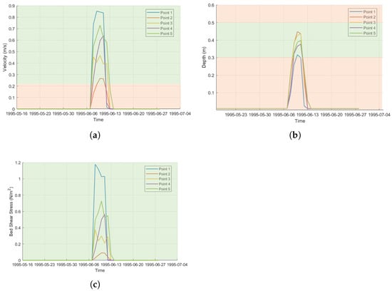
Figure 9.
(a) Velocity for observation points at low flow in upstream area with critical limits for spawning habitats (b). Water depth for observation points at low flow in upstream area with critical limits for spawning area. (c) Bed shear stress with critical limits in colors; green to red for gravel size of 16 mm.
The downstream area was also examined using five observation points, positioned as shown in Figure 6b. As in the other study areas, bed shear stress remained low at all points; see Figure 10c. Water velocities also did not reach critical levels during the high-flow event, as illustrated in Figure 10a. The main limiting factor in this area is water depth—suitable habitat zones remain dry except during the peak of the high-flow period, as shown in Figure 10b.

Figure 10.
(a) Velocity for observation points at low flow in upstream area with critical limits for spawning habitats. (b). Water depth for observation points at low flow in upstream area with critical limits for spawning area. (c) Bed shear stress with critical limits in colors; green to red for gravel size of 16 mm.
These results demonstrate that grayling spawning habitats are highly sensitive to large fluctuations in flow conditions. If spawning occurs in areas that initially experienced lower water velocities and depths, there is a significant risk that reproduction will be impaired in years with extreme flow events.
These findings also underscore the importance of not only identifying suitable habitats spatially but also ensuring their availability over time. Management strategies aimed at supporting grayling populations should therefore consider flow regulation or restoration efforts that extend the duration of suitable hydraulic conditions, especially during key reproductive windows.
4. Discussion
The study shows that water velocities and water depths vary significantly during an extreme event. If such an event occurs during a critical period when grayling are in their reproductive stage, they are more sensitive to these changes.
Water velocities are difficult to influence due to the natural characteristics of the area close to the discharge outlet, but the power companies have the opportunity to minimize the ecological impact by carefully managing how the downstream water level is utilized. By managing the downstream water level to change more gradually, the impact can be minimized.
If a high flow occurs suddenly during the spawning period, when grayling are still in their eggs and fry stage, they have a harder time adapting to the high flow. To some extent, hydropower plants can influence how the spring flood passes through the plants, thus minimizing the impact of extreme events.
This study does not address stranding risk, as the available data are based on daily discharge values and thus do not capture rapid flow reductions or zero-flow events downstream. This is a well-documented issue that has been studied [38,39], and it warrants further investigation in this section of the river. To better understand the risk of stranding, high-resolution flow data (e.g., hourly) would be required. Additionally, longer periods of drought are expected under projected climate change scenarios. Therefore, it is recommended to analyze the occurrence and impact of zero-flow periods and explore how hydropower operations could be optimized on a yearly scale—such as conserving spring flows—as proposed by [40] in the context of salmonid habitats.
Even natural watercourses are subject to substantial spring floods, which are not necessarily detrimental. In fact, many riparian zones benefit from periodic inundation, as it contributes to increased biological diversity [41]. However, in regulated rivers where strict limitations are imposed on reservoir water levels due to dam safety requirements, such floodplain connectivity is often restricted.
Due to strict regulations governing water levels in impounded rivers, the water surface is not expected to rise significantly above the upper limit, even during extreme flow events. This, in turn, may reduce the impact of such events on the local people. However, the recreational value of the area has been considerably affected by the river impoundment, and the ecological status of the region has declined since the installation of the hydropower plants.
A previous study comparing steady-state and transient flow simulations found that bed shear stress was slightly underestimated in the upstream section and overestimated in the downstream section [26]. Since the present study is based solely on daily mean values, it does not capture the full range of peak flow velocities and associated bed shear stress. This presents certain challenges when conducting long-term simulations. Due to computational limitations, it is not feasible to capture all fine-scale details, resulting in some loss of information. However, gaining an understanding of how seasonal variations may evolve over time is also important, which justifies the use of coarser simulations. The present study focuses solely on variations during an extreme spring flood event. Nonetheless, it would be valuable to investigate how seasonal flow patterns may be affected by climate change. By employing a coarser mesh, larger time steps, and steady-state simulations, it would be possible to identify long-term trends in flow dynamics.
Climate change is expected to affect not only the magnitude of river discharge but also the temperature of the water flow, both of which will have implications for the riverine ecosystem. Although not addressed in this study, water temperature is an important factor that should be considered in future research. Changes in temperature patterns will also influence the timing of ice breakup, which in turn may have additional consequences. Large volumes of ice and debris transported during breakup events can significantly impact shear stress and sediment transport dynamics. In the present model, only the water flow is considered.
As the impacts of climate change are becoming increasingly evident even in northern regions, it is important to investigate how future changes may affect these areas in order to help minimize ecological impacts—particularly in rivers already negatively influenced by hydropower development. This study is based on a historical event, which is used as a worst-case scenario to analyze potential consequences if similar events were to occur more frequently. While it would have been advantageous to use a more detailed and updated climate model for the region to obtain more accurate projections of future climate impacts, this study provides an initial analysis based on the best available data at the time.
5. Conclusions
Water depths and flow velocities vary significantly during extreme flow events. Previously suitable spawning habitats may become submerged under deeper water, and flow velocities increase. As a result, the time window during which an area remains suitable for spawning is shortened. Moreover, the rapid changes in hydraulic parameters within a short period can have critical implications for the reproductive success of grayling.
The results indicate that bed shear stress does not increase significantly beyond levels that can occur under other flow conditions when water levels are low and discharge is high. This suggests that sediment transport occurs continuously in the river across various flow regimes. The most critical period is when grayling are in their most vulnerable life stages, such as during egg incubation or larval development, as water velocities can become exceptionally high. Once grayling have grown larger, they are less sensitive to high water velocities and are capable of returning to preferred habitats once peak flow conditions subside.
Eggs may be particularly vulnerable if water levels rise significantly, as this can alter temperature regimes and increase sediment transport. Importantly, during elevated downstream water levels, bed shear stress does not appear to reach critically high values in spawning areas, even under high-flow conditions.
To enhance the understanding of how climate change may affect the area, a more detailed climate analysis of the specific region would have been valuable. Such an analysis could contribute to more accurate assessments of future hydrological changes and their potential impacts on local ecosystems.
Author Contributions
Conceptualization, M.L.S., A.G.A. and J.G.I.H.; methodology, M.L.S., A.G.A. and J.G.I.H.; software, M.L.S.; formal analysis, M.L.S.; investigation, M.L.S.; resources, A.G.A.; writing—original draft preparation, M.L.S.; writing—review and editing, A.G.A., J.G.I.H. and J.A.; visualization, M.L.S.; supervision, A.G.A. and J.G.I.H.; project administration, A.G.A. and J.G.I.H.; funding acquisition, A.G.A. and J.G.I.H. All authors have read and agreed to the published version of the manuscript.
Funding
This work is a part of the Re-Hydro project funded by the EU program Interreg Aurora (Grant number 20358005).
Data Availability Statement
The raw data supporting the conclusions of this article will be made available by the authors upon request.
Acknowledgments
The authors wish to thank Frida Niemi for providing the model validation data and for her valuable expertise in the modeled area.
Conflicts of Interest
The authors declare that the research was conducted in the absence of any commercial or financial relationships that could be construed as a potential conflict of interest.
References
- Schneider, C.; Laize, C.L.R.; Acreman, M.C.; Floerke, M. How will climate change modify river flow regimes in Europe? Hydrol. Earth Syst. Sci. 2013, 17, 325–339. [Google Scholar] [CrossRef]
- IPCC; Solomon, S.; Qin, D.; Manning, M.; Chen, Z.; Marquis, M.; Averyt, K.; Tignor, M.; Miller, H. Summary for Policymakers: Climate Change 2007: The Physical Science Basis. Contribution of Working Group III to the Fourth Assessment Report of the Intergovernmental Panel on Climate Change; Cambridge University Press: Cambridge, UK, 2007. [Google Scholar]
- Hirabayashi, Y.; Kanae, S.; Emori, S.; Oki, T.; Kimoto, M. Global projections of changing risks of floods and droughts in a changing climate. Hydrol. Sci. J. 2008, 53, 754–772. [Google Scholar] [CrossRef]
- Döll, P.; Schmied, H.M. How is the impact of climate change on river flow regimes related to the impact on mean annual runoff? A global-scale analysis. Environ. Res. Lett. 2012, 7, 014037. [Google Scholar] [CrossRef]
- Donnelly, C.; Greuell, W.; Andersson, J.; Gerten, D.; Pisacane, G.; Roudier, P.; Ludwig, F. Impacts of climate change on European hydrology at 1.5, 2 and 3 degrees mean global warming above preindustrial level. Clim. Change 2017, 143, 13–26. [Google Scholar] [CrossRef]
- Arheimer, B.; Lindström, G. Climate impact on floods: Changes in high flows in Sweden in the past and the future (1911–2100). Hydrol. Earth Syst. Sci. 2015, 19, 771–784. [Google Scholar] [CrossRef]
- Knouft, J.H.; Ficklin, D.L. The Potential Impacts of Climate Change on Biodiversity in Flowing, Freshwater Systems. Annu. Rev. Ecol. ESyst. 2017, 48, 111–133. [Google Scholar] [CrossRef]
- Heino, J.; Virkkala, R.; Toivonen, H. Climate change and freshwater biodiversity: Detected patterns, future trends and adaptations in northern regions. Biol. Rev. 2009, 84, 39–54. [Google Scholar] [CrossRef]
- Wasti, A.; Ray, P.; Wi, S.; Folch, C.; Ubierna, M.; Karki, P. Climate change and the hydropower sector: A global review. Wiley Interdiscip. Rev. Clim. Change 2022, 13, e757. [Google Scholar] [CrossRef]
- Uvo, C.B.; Berndtsson, R. North Atlantic Oscillation; a climatic indicator to predict hydropower availability in Scandinavia. Hydrol. Res. 2002, 33, 415–424. [Google Scholar] [CrossRef]
- Renöfält, B.M.; Jansson, R.; Nilsson, C. Effects of hydropower generation and opportunities for environmental flow management in Swedish riverine ecosystems. Freshw. Biol. 2010, 55, 49–67. [Google Scholar] [CrossRef]
- Charles, S.; Mallet, J.-P.; Persat, H. Population dynamics of grayling: Modelling temperature and discharge effects. Math. Model. Nat. Phenom. 2006, 1, 31–48. [Google Scholar] [CrossRef]
- Wedekind, C.; Kueng, C. Shift of spawning season and effects of climate warming on developmental stages of a grayling (Salmonidae). Conserv. Biol. 2010, 24, 1418–1423. [Google Scholar] [CrossRef]
- Hajdukiewicz, H.; Wyżga, B.; Amirowicz, A.; Oglęcki, P.; Radecki-Pawlik, A.; Zawiejska, J.; Mikuś, P. Ecological state of a mountain river before and after a large flood: Implications for river status assessment. Sci. Total Environ. 2018, 610–611, 244–257. [Google Scholar] [CrossRef]
- Reich, P.; Lake, P.S. Extreme hydrological events and the ecological restoration of flowing waters. Freshw. Biol. 2015, 60, 2639–2652. [Google Scholar] [CrossRef]
- Walker, R.H.; Naus, C.J.; Adams, S.R. Should I stay or should I go: Hydrologic characteristics and body size influence fish emigration from the floodplain following an atypical summer flood. Ecol. Freshw. Fish 2022, 31, 607–621. [Google Scholar] [CrossRef]
- Merz, R.; Blöschl, G. A process typology of regional floods. Water Resour. Res. 2003, 39, 11–18. [Google Scholar] [CrossRef]
- Blöschl, G.; Hall, J.; Parajka, J.; Perdigão, R.A.P.; Merz, B.; Arheimer, B.; Aronica, G.T.; Bilibashi, A.; Bonacci, O.; Borga, M.; et al. Changing climate shifts timing of European floods. Science 2017, 357, 588–590. [Google Scholar] [CrossRef]
- Niemi, F.M.; Andersson, A.G.; Hellström, J.G.I. An ecohydraulic approach for 2D hydraulic modelling of a regulated river reach. In Proceedings of the 8th IAHR Europe Congress, Lisbon, Portugal, 4–7 June 2024. [Google Scholar]
- Niemi, F.M.; Andersson, A.G.; Hellström, J.G.I.; Hajiesmaeili, M.; Aldvén, D. Hydraulic modelling of bedload transport to support restoration locations of spawning habitats in a regulated river. Water 2025. Details pending publication. [Google Scholar]
- Andersson, A.G.; Lycksam, H. Hydraulic modelling of a regulated river reach on different scales to evaluate its inherent environment conditions. In Proceedings of the 39th IAHR World Congress, Granada, Spain, 19–24 June 2022. [Google Scholar]
- Berga, L. The Role of Hydropower in Climate Change Mitigation and Adaptation: A Review. Engineering 2016, 2, 313–318. [Google Scholar] [CrossRef]
- Swedish Meteorological and Hydrological Institute (SMHI). 1995—Extrem Vårflod i Norra Sverige. Available online: https://www.smhi.se/kunskapsbanken/hydrologi/historiska-oversvamningar/1995—Extrem-varflod-i-norra-sverige (accessed on 29 April 2025).
- Deltares. D-Flow Flexible Mesh, User Manual; Deltares: Delft, The Netherlands, 2024. [Google Scholar]
- Swedish Meteorological and Hydrological Institute (SMHI). Hydrological Observations. Available online: https://teams.microsoft.com/l/message/19:45a73e11-840f-47af-ace7-7b25f64d6e4e_a15c0607-52f6-4bc7-8bc2-3a9f809f661d@unq.gbl.spaces/1753502854019?context=%7B%22contextType%22%3A%22chat%22%7D (accessed on 1 November 2024).
- Niemi, F.M.; Andersson, A.G.; Hellström, J.G.I.; Hajiesmaeili, M.; Aldvén, D. Investigating Steady-State Interpolation and Transient Hydraulic Modelling to Evaluate European Grayling Habitat in a Hydropeaking River. Water 2025, 17, 1083. [Google Scholar] [CrossRef]
- Nykänen, M.; Huusko, A.; Mäki-Petäys, A. Seasonal changes in the habitat use and movements of adult European grayling in a large subarctic river. J. Fish Biol. 2001, 58, 506–519. [Google Scholar] [CrossRef]
- Nykänen, M.; Huusko, A. Size-related changes in habitat selection by larval grayling (Thymallus thymallus L.). Ecol. Freshw. Fish 2003, 12, 127–133. [Google Scholar] [CrossRef]
- Nykänen, M.; Huusko, A. Transferability of habitat preference criteria for larval European grayling (Thymallus thymallus). Can. J. Fish. Aquat. Sci. 2004, 61, 185–192. [Google Scholar] [CrossRef]
- Gönczi, A.P. A study of physical parameters at the spawning sites of the European grayling (Thymallus thymallus L.). Regul. Rivers: Res. Manag. 1989, 3, 221–224. [Google Scholar] [CrossRef]
- Bakken, T.H.; Forseth, T.; Harby, A.; Alfredsen, K.; Arnekleiv, J.V.; Berg, O.K.; Casas-Mulet, R.; Charmasson, J.; Greimel, F.; Halley, D.; et al. Miljøvirkninger av Effektkjøring: Kunnskapsstatus og råd til Forvaltning og Industri; Norsk Institutt for Naturforskning: Trondheim, Norway, 2016. [Google Scholar]
- Young, P.S.; Cech, J.J.; Thompson, L.C. Hydropower-related pulsed-flow impacts on stream fishes: A brief review, conceptual model, knowledge gaps, and research needs. Rev. Fish Biol. Fish. 2011, 21, 713–731. [Google Scholar] [CrossRef]
- Moreira, M.; Hayes, D.S.; Boavida, I.; Schletterer, M.; Schmutz, S.; Pinheiro, A. Ecologically-based criteria for hydropeaking mitigation: A review. Sci. Total Environ. 2019, 657, 1508–1522. [Google Scholar] [CrossRef]
- Hayes, D.S.; Hauer, C.; Unfer, G. Fish stranding in relation to river bar morphology and baseflow magnitude: Combining field surveys and hydrodynamic numerical modelling. Ecohydrology 2024, 17, e2616. [Google Scholar] [CrossRef]
- Malcolm, I.A.; Gibbins, C.N.; Soulsby, C.; Tetzlaff, D.; Moir, H.J. The influence of hydrology and hydraulics on salmonids between spawning and emergence: Implications for the management of flows in regulated rivers. Fish. Manag. Ecol. 2012, 19, 464–474. [Google Scholar] [CrossRef]
- Casas-Mulet, R.; Saltveit, S.J.; Alfredsen, K. The survival of Atlantic salmon (Salmo salar) eggs during dewatering in a river subjected to hydropeaking. River Res. Appl. 2015, 31, 433–446. [Google Scholar] [CrossRef]
- McMichael, G.A.; Rakowski, C.L.; James, B.B.; Lukas, J.A. Estimated fall Chinook salmon survival to emergence in dewatered redds in a shallow side channel of the Columbia River. N. Am. J. Fish. Manag. 2005, 25, 876–884. [Google Scholar] [CrossRef]
- Auer, S.; Zeiringer, B.; Fuhrer, S.; Tonolla, D.; Schmutz, S. Effects of river bank heterogeneity and time of day on drift and stranding of juvenile European grayling (Thymallus thymallus L.) caused by hydropeaking. Sci. Total Environ. 2017, 575, 1515–1521. [Google Scholar] [CrossRef]
- Hauer, C.; Schmalfuss, L.; Unfer, G.; Schletterer, M.; Fuhrmann, M.; Holzapfel, P. Evaluation of the potential stranding risk for aquatic organisms according to long-term morphological changes and grain size in alpine rivers impacted by hydropeaking. Sci. Total Environ. 2023, 883, 163667. [Google Scholar] [CrossRef]
- Sundt-Hansen, L.; Hedger, R.D.; Ugedal, O.; Diserud, O.H.; Finstad, A.G.; Sauterleute, J.F.; Tøfte, L.; Alfredsen, K.; Forseth, T. Modelling climate change effects on Atlantic salmon: Implications for mitigation in regulated rivers. Sci. Total Environ. 2018, 631, 1005–1017. [Google Scholar] [CrossRef]
- Andersson, E.; Nilsson, C.; Johansson, M.E. Plant dispersal in boreal rivers and its relation to the diversity of riparian flora. J. Biogeogr. 2000, 27, 1095–1106. [Google Scholar] [CrossRef]
Disclaimer/Publisher’s Note: The statements, opinions and data contained in all publications are solely those of the individual author(s) and contributor(s) and not of MDPI and/or the editor(s). MDPI and/or the editor(s) disclaim responsibility for any injury to people or property resulting from any ideas, methods, instructions or products referred to in the content. |
© 2025 by the authors. Licensee MDPI, Basel, Switzerland. This article is an open access article distributed under the terms and conditions of the Creative Commons Attribution (CC BY) license (https://creativecommons.org/licenses/by/4.0/).