Article

Modelling of Water Level Fluctuations and Sediment Fluxes in Nokoué Lake (Southern Benin)

by
Tètchodiwèï Julie-Billard Yonouwinhi
1,2,3,
Jérôme Thiébot
4,*,
Sylvain S. Guillou
4,
Gérard Alfred Franck Assiom d’Almeida
3 and
Felix Kofi Abagale
5
1
Laboratory of Applied Hydrology (LHA), National Institute of water (INE), African Center of Excellence for Water and Sanitation (C2EA), University of Abomey-Calavi (UAC), Cotonou 01 BP 4521, Benin
2
International Chair in Mathematical Physics and Applications (ICMPA–UNESCO Chair), University of Abomey-Calavi (UAC), Cotonou 072 BP 50, Benin
3
Laboratory of Geology, Mining and Environment (LGME), Faculty of Science and Technology (FAST), University of Abomey-Calavi (UAC), Cotonou 01 BP 526, Benin
4
LUSAC UR 4253, University of Caen Normandy, 60 rue Max-Pol Fouchet, F-50130 Cherbourg en Cotentin, France
5
West African Center for Water, Irrigation and Sustainable Agriculture, University for Development Studies, Tamale Box TL1350, Northern Region, Ghana
*
Author to whom correspondence should be addressed.
Water 2025, 17(15), 2209; https://doi.org/10.3390/w17152209
Submission received: 17 June 2025 / Revised: 19 July 2025 / Accepted: 20 July 2025 / Published: 24 July 2025

Abstract

Nokoué Lake is located in the south of Benin and is fed by the Ouémé and Sô Rivers. Its hydrosedimentary dynamics were modelled using Telemac2D, incorporating the main environmental factors of this complex ecosystem. The simulations accounted for flow rates and suspended solids concentrations during periods of high and low water. The main factors controlling sediment transport were identified. The model was validated using field measurements of water levels and suspended solids. The results show that the north–south current velocity ranges from 0.5 to 1 m/s during periods of high water and 0.1 to 0.5 m/s during low-water periods. Residual currents are influenced by rainfall, river discharge, and tides. Complex circulation patterns are caused by increased river flow during high water, while tides dominate during low water and transitional periods. The northern, western, and south-eastern parts of the lake have weak residual currents and are, therefore, deposition zones for fine sediments. The estimated average annual suspended solids load for 2022–2023 is 17 Mt. The model performance shows a strong agreement between the observed and simulated values: R2 = 0.91 and NSE = 0.93 for water levels and R2 = 0.86 and NSE = 0.78 for sediment transport.

1. Introduction

The ecosystems of lakes, particularly those in tropical zones, are strongly influenced by seasonal climate variations. Nokoué Lake in Benin is an example of a lake where these variations cause significant hydrological changes and alter sediment flows [1]. Intensive use of the land around these bodies of water affects the surface water quality, which has become a receptacle for various anthropogenic effluents [2,3,4,5]. These ecosystems are among the world’s most productive and provide vital services that support various activities such as aquaculture, fishing, recreation, tourism, sand extraction and transportation [6,7].
Fluctuations in water levels and sediment fluxes are complex, dynamic processes that play a crucial role in the evolution of lake environments. Previous studies [8] have shown that seasonal variations in water levels influence sediment transport processes and spatial distribution.
The transport and deposition of suspended solids (SS) play a crucial role in the redistribution of sediments between watersheds, lake environments, and marine ecosystems [9,10]. It is important to understand and predict sediment dynamics in order to assess changes in sediment characteristics or evaluate anthropogenic impacts [11,12]. In the case of Nokoué Lake, the erosion of the tributary banks and wind-induced resuspension of sediments are major processes during the flood season. However, these investigations are currently based on sporadic observations. Nevertheless, our overall understanding of sediment dynamics and SS in the lake remains limited. Due to rainwater runoff, sediments from rivers and watersheds are often transported to the lake. The remobilization of sediments from the lake bed during continental inflows can affect water quality and contribute to the lake filling up. One of the key mechanisms identified is the fluctuation of water levels and sediment fluxes in Nokoué Lake and its channels [13].
Numerous studies have been carried out over the past few decades to elucidate the general hydro-ecological functioning of Nokoué Lake (see [14], for a review). Field campaigns conducted by [15] in 2015 demonstrated that water turbidity and suspended solids (SS) concentrations were high in the eastern part of the lake, peaking in September during the flood season. Since late 2017, a multidisciplinary observation program has been in place at Nokoué Lake, enabling systematic and continuous data collection and improving our understanding of this ecosystem [13,16,17,18]. Previous studies have used numerical models to simulate sediment transport processes, often incorporating in situ and satellite data to calibrate and validate these models [19]. Commonly employed analytical methods include hydrodynamic and sediment modelling and remote sensing [20]. For instance, 2D and 3D hydrodynamic models such as HEC-RAS and Telemac have been used to simulate water flows and sediment transport in various lake and river environments [21]. These models enable the representation of complex interactions between currents, water levels, and sediment deposition. Recent studies on hydrosedimentary processes have elucidated various factors influencing sediment dynamics in lake and estuarine systems. Hydrodynamic models have been used to demonstrate the central role of precipitation and fluvial inputs in sediment transport [22]. Isotopic tracers have been used to discern seasonal variations in sediment sources [23]. Remote sensing techniques were combined with modelling to analyze the effect of seasonal water level variations on sediment distribution [24]. In situ and satellite-derived data have been integrated into numerical models to study the interactions between river inputs, tides, and winds [25].
This study aims to understand and quantify the complex dynamics of water and suspended solids fluxes in Nokoué Lake, a vital ecosystem in southern Benin, under the combined influence of river inflows, precipitation, and tides, in the context of strong seasonal variability and increasing the anthropogenic impact. More specifically, the study aims to decipher the hydrological and sedimentary mechanisms governing Nokoué Lake; develop robust and reliable modelling tools to simulate these dynamics; and address the existing data and modelling gaps regarding suspended solids (SS) in this type of West African lagoonal system.

2. Materials and Methods
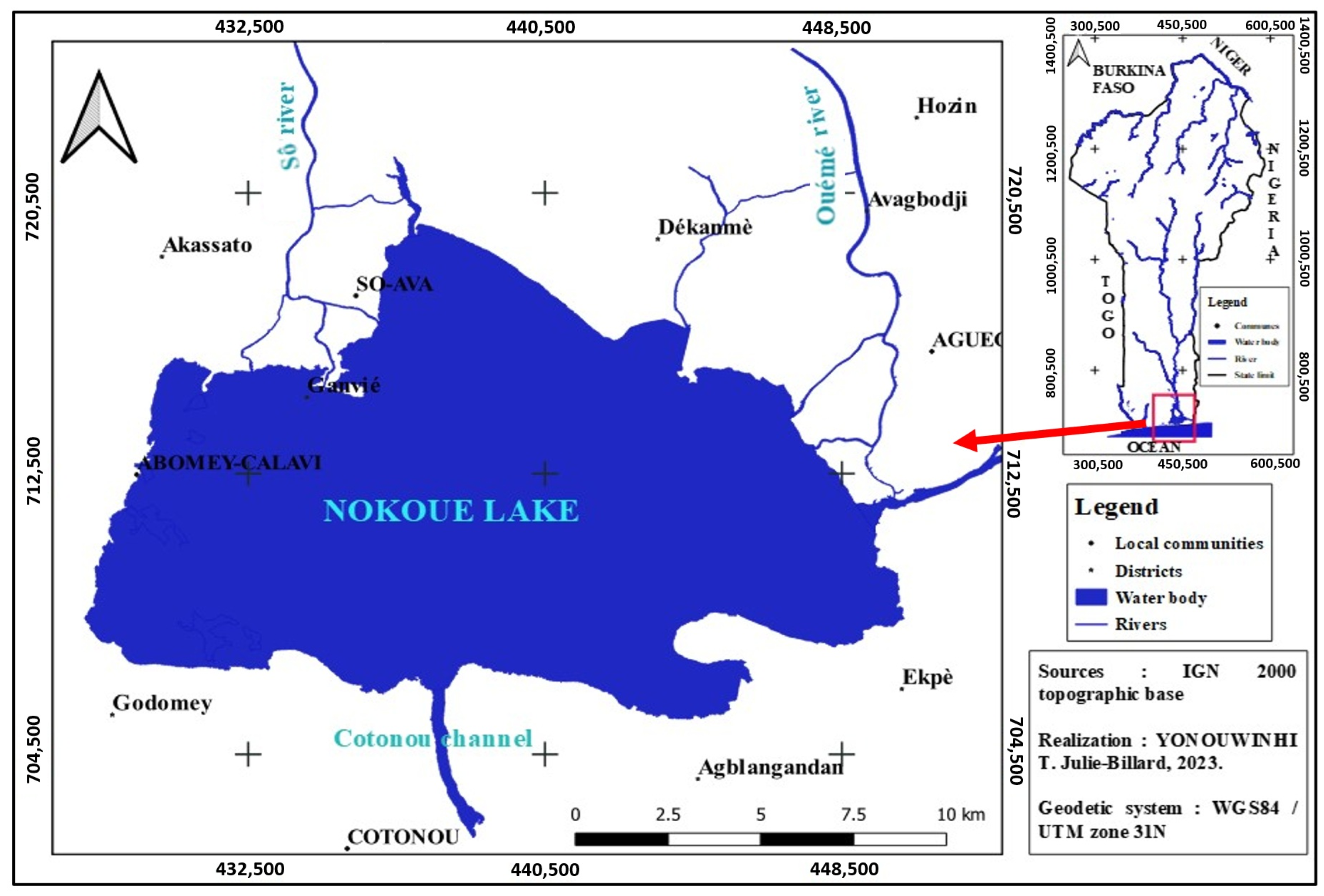
2.1. Study Area

Nokoué Lake, the largest in Benin, stretches 20 km from west to east and 11 km from south to north [26,27]. It has an average depth of 1.3 m and 2.2 m during the low- and high-water seasons, respectively [16]. The maximum depths are found in the Cotonou channel, where they exceed 5 m.
It is the largest brackish water body in Benin, covering an area of 150–170 km2 during the dry and the rainy seasons, with a volume of 1.5 × 10⁸ m3 during low-water periods [27]. The lake is connected to the Atlantic Ocean via the Cotonou Channel, which is approximately 4.5 km long and 400 m wide (see Figure 1). The semi-diurnal tidal amplitude is strongly attenuated within the lake. It ranges from 0.55 to 0.90 m in the ocean to 0.03 to 0.05 m inside the lake [16]. The lake receives freshwater from multiple sources; the main ones are the Sô and Ouémé rivers in the north of the lake (Figure 1). These rivers have watersheds of 1000 km2 and 50,000 km2, respectively [14,27]. Additionally, small amounts of fresh water enter the lake from the Djonou River, which is located southwest of the area, and the Totchè Canal [14,26,27]. The lake also receives large quantities of domestic effluents linked to the activities of nearby populations. The seasonal cycle of the regional climate is dominated by the West African monsoon [28], which is characterized by two dry seasons and two rainy seasons [29,30,31].
The short dry season runs from August to September, while the long dry season runs from December to February [31]. The main rainy season runs from March to July, peaking in June, while the short rainy season runs from September to November [29,30]. The average annual rainfall is around 1300 mm [32,33,34]. However, it is important to note that these two rainy seasons do not significantly affect the water level of Nokoué Lake [16]. Conversely, the water level is strongly influenced by the discharge of water from the Ouémé and Sô watersheds in the north of Benin. In the area north of the lake, a single rainy season runs from April to October, with the heaviest rainfall occurring in August [29,30,32,33]. During this period, the lake’s water level rises by around 1 m [16], and a peak in suspended solids entering the lake is observed in July. Thus, the lagoon’s hydrological regime is mainly influenced by seasonal variations in river flows. Unfortunately, there are no direct measurements of river flows into lake Nokoué, and estimates of maximum flows during the rainy season vary considerably, ranging from approximately 400 to 1000 m3/s [27,33,35]. Ref. [13] recently studied the evolution of water levels in tidal lakes and found a maximum net flux of approximately 1100 m3/s.
The prevailing winds in the study area are characterized by southwesterly winds blowing in from the ocean throughout the year. However, during the long dry season, northeasterly winds called Harmattan can blow episodically from December to March [31,36]. The average monthly wind speed ranges from 2 to 5 m/s, with a peak primarily in August and secondarily in March [31]. Eighty per cent of suspended solids are transported during the first rainy season (July 2022), from the south of the country and at the start of the rainy season in the north. Indeed, flows are relatively low in November and March, corresponding to low concentrations of suspended solids. This indicates that sediment transport in the dry season is influenced by the tide and wind, as river flows are zero.

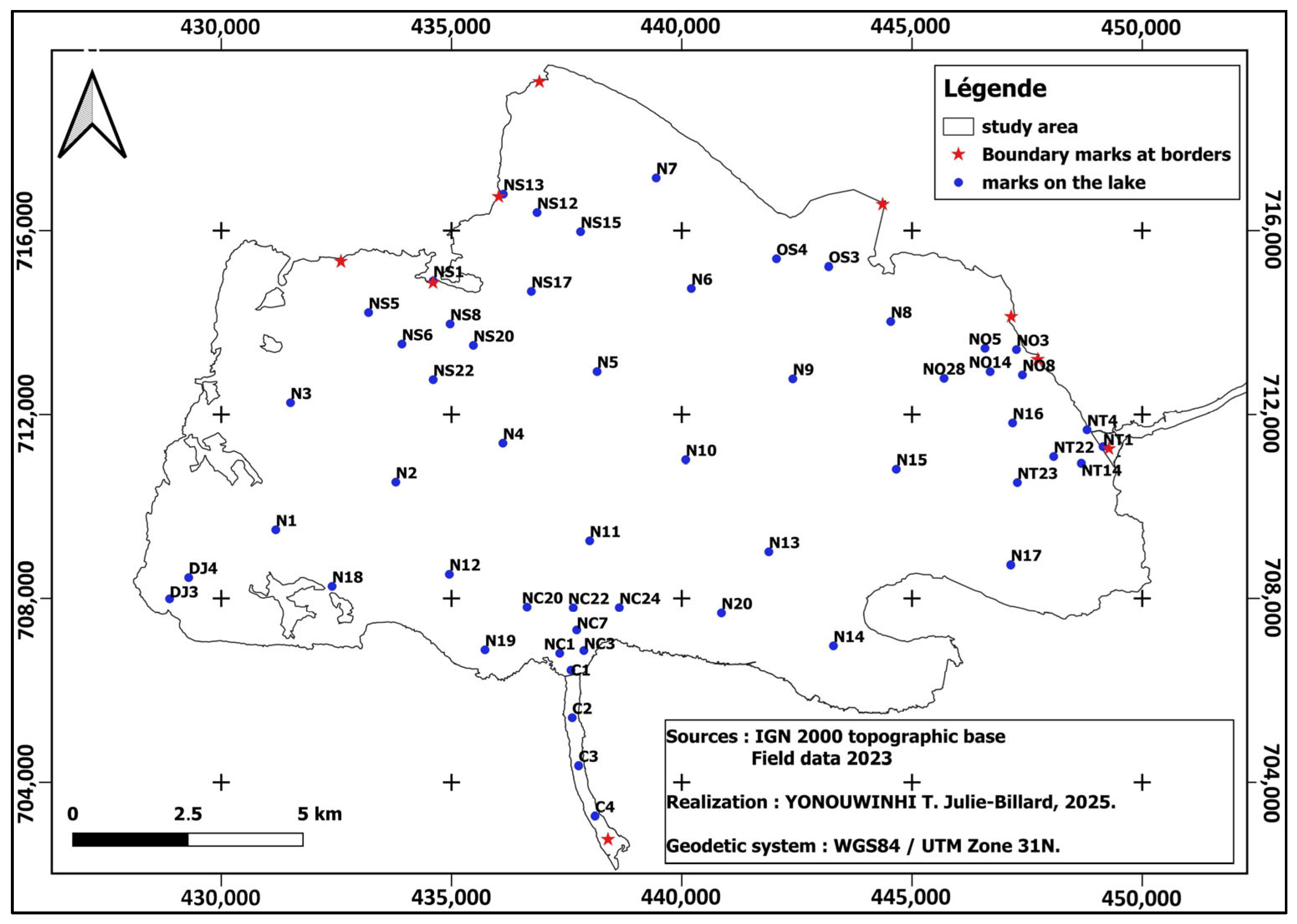
2.2. Field Measurements

Field measurements were carried out in July and September 2022, as well as in November 2022, March 2023, and June 2023. The objective during these campaigns was to collect bathymetric data, water levels, flow rates, current velocities, and SS concentrations. The bathymetric data was measured using a Garmin 521s dual-frequency echo sounder operating at approximately 200 kHz. The water levels, flow rates, current velocities were measured with a Rio Grande Acoustic Doppler Current Profiler (ADCP) current meter is equipped with four acoustic transducers that emit at a frequency of 1200 kHz. The Win River 2 software automatically calculates the results in real time. The suspended solids measurement protocol, which is in accordance with the European standard NF EN 872, was used to measure SS concentrations. These measurements were taken on the lake and its main tributaries. Data from the tide gauge at the Autonomous Port of Cotonou for 2022 were also used for tidal forecasts. Figure 2 shows the various measurement points on the lake.

2.3. Model Description

The lake hydrodynamic was simulated using Telemac2D (v8p3r1), which solves the shallow water equations. Water Equation (1) uses a finite element approach [37,38].
h t + u · h + h   d i v u = s h u t + u · u = g z x + 1 h d i v ( h v t u ) + s x v t + u · v = g z y + 1 h d i v ( h v t v ) + s y
where h (m) is the water depth; u, v (m/s) are the depth-averaged velocity components; g (m/s2) is the gravity acceleration; v t (m2/s) is the momentum diffusion coefficient; Z (m) is the free surface elevation; t (s) is the time; x, y (m) are the horizontal space components; s h (m/s) is the fluid source or sink (a source term, which represents mass inputs or losses independent of the flow dynamics); s x , s y (m/s2) are source or sink terms for the momentum equations (wind, Coriolis force, and bottom friction).
Figure 3a shows the mesh, which is made up of 52,079 nodes and 102,150 elements. The mesh size varies between 10 and 100 m, and the bathymetry data was acquired from 50,477 boreholes in March 2023 (see Figure 3a). Turbulence is accounted for using the k-ε model. Strickler’s law is used to model friction on the bottom, with a coefficient of friction of 50 m1/3/s. The time step is 1 s, corresponding to a CFL number of less than 0.3.
The transport of suspended cohesive solids is modelled using the GAIA code, which is coupled to Telemac2D. This code solves the advection–diffusion Equation (2).
h C t + h u C x + h v C y = x h ε s C x + y h ε s C y + E D
where C = C(x,y,t) is the SS concentration (g/L), ε s is a diffusion coefficient, E is erosion (m), and D is deposition (m).
Erosion and deposition fluxes [39,40] are calculated using the formulations of [41] and [42].
E = M τ b τ c e 1   i f   τ b > τ c e 0   o t h e r w i s e
where M is the constant of the Krone–Partheniades erosion law (kg/m2/s) and τ c e is the critical erosion stress (N/m2), and τ b is the bottom shear stress (N/m2).
D = W s C 1 τ b / ρ U * c r 2 ,
where W s is the settling velocity (m/s); C is the concentration of SS in the water column (g/L); U * c r is the critical shear velocity for mud deposition, expressed in (m/s) and calculated as follows τ b / ρ ; and ρ is the density of water (kg/m3).
It is calculated using [43] formula, as described by [40].
W s = s 1 g d 2 18 v i f d 10 4 10 v / d 1 + 0.01 s 1 g d 3 v 2 1 i f 10 4 < d < 10 3 1.1 s 1 g d o t h e r w i s e .
where s is the relative density of the sediment (kg/m3); ν is the kinematic viscosity of the fluid (m2/s); and d is the diameter of the sediment particles (m).

2.4. Setting Up the Model

The boundary conditions for the hydrodynamic model are the flow rates and water levels. For the sediment model, the boundary conditions are the suspended solids (SS) concentrations for the 2022 and 2023 seasons. These SS values are based on specific data collected during each season. Water flows and heights are imposed at different inlets, as shown in Figure 3a,b.
At the southern boundary (Cotonou Channel), water levels are controlled by the tide. Level predictions are obtained using Matlab R2017b software under UTIDE command “Unequally spaced Time series Inference and Decomposition” (ut_solv and ut_reconstr). Fifteen tidal constituents (M2, S2, N2, K2, K1, O1, P1, Q1, MM, MF, M4, MN4, MS4, 2N2, and S1) were identified using data from the Cotonou tide gauge. Water levels have also been imposed at Totché, to the east of the lake. Flow rates have been imposed at the Sô and Ouémé rivers, which are located to the north of the lake. These values are based on measurements taken at various times throughout the year.
In the absence of permanent upstream gauging stations, the model boundary inflows were based on spot flow rate measurements collected during five field campaigns between July 2022 and June 2023, which covered both the dry and wet seasons. These flow rates were considered to be representative of suspended solids contribution. Monthly hydrographs were reconstructed using linear interpolation between measurement dates. Seasonal rainfall trends and regional hydrological knowledge were employed to ensure temporal consistency and plausible flow dynamics. Table 1 summarizes the discharge values imposed at each boundary section.
Calibrating and validating the model consisted of comparing the simulated water levels with measurements. Water level predictions were averaged over 50 points distributed across the lake. Then, they were compared to the measurements over a six-day period during a period of low water. The hydrodynamic and sedimentary models were calibrated and validated using data acquired between July 2022 and June 2023. For each year, the models simulated the different periods corresponding to our field campaigns. We calibrated Telemac2D (v8p3r1) by adjusting the Strickler (bottom friction) coefficients. This was carried out in order to minimize the error between the model predictions and the measurements of the water level and flow. We then calibrated the GAIA model by testing different values of critical erosion stress ( τ c e ), critical shear rate for deposition ( U * c r ), sediment particle settling velocity ( W s ), and the Krone–Partheniades erosion constant (M). This was done to minimize the error between model predictions and measurements of SS concentration. The initial selections for these parameters were based on earlier work, as shown in Table 2. After several tests, we opted for the following values: τ c e = 0.2 N/m2, U * c r = 1.0 m/s, and M = 2.0 10−5 kg/(s.m2) [44].

2.5. Model Performance Indicators

Several criteria were used to assess the model performance. These are the coefficient of determination (R2), the Nash coefficient, and the root mean square error (RMSE). The closer the R2 is to 1 and the RMSE is to 0, the better the model. Similarly, the closer the RMSE is to 0, the closer the simulations are to the observations.
R 2 = i = 1 n X o b s , i X ¯ o b s . X m o d e l , i X ¯ m o d e l 2 i = 1 n X o b s , i X ¯ o b s 2 . i = 1 n X m o d e l , i X ¯ m o d e l 2
N S E = 1 i = 1 n X o b s , i X m o d e l 2 i = 1 n X o b s , i X o b s ¯ 2
X o b s is the observed data, X m o d e l is the simulated data, and X o b s is the mean of the observations. n is the total number of observations.
R M S E = i = 1 n X o b s , i X m o d e l 2 n

3. Results

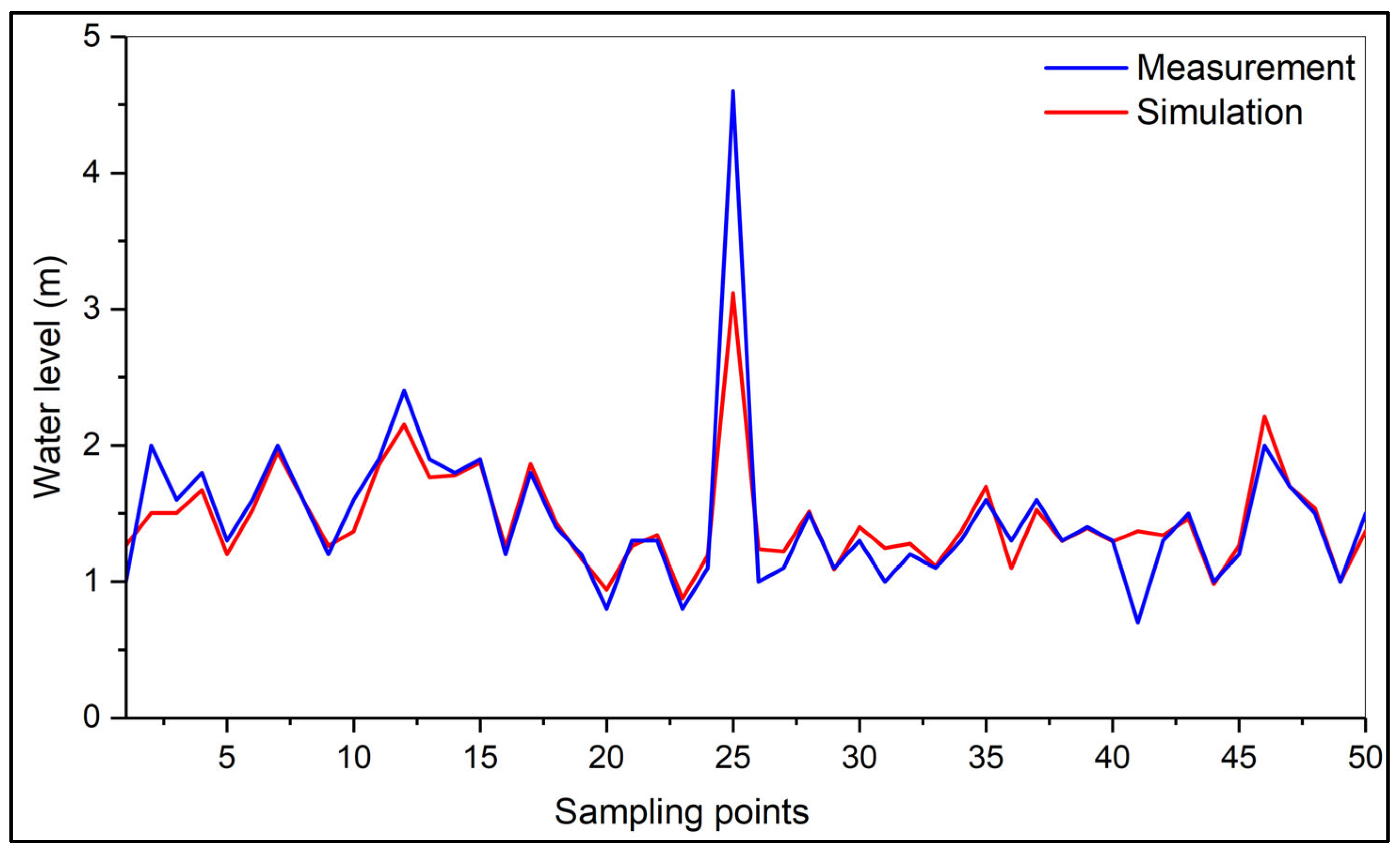
3.1. Calibration and Validation of the Hydrodynamic Model

Figure 4 shows the comparison between the measured and modelled averaged water elevations, over 50 locations in the lake (see Figure 2) 4.
This figure shows that the model can reproduce the lake water level fluctuations during high and low tides (the low season). This is corroborated by the high coefficients of determination (0.86 and 0.78 for the Nash coefficient, see Table 3) for calibration.
For validation purposes, Figure 5 illustrates the correlation between the measured and simulated water levels in Lake Nokoué over several months of the year. The data show a strong correlation, confirmed by the high correlation and determination coefficients of 0.91. The figure shows that the highest water levels are observed in November and June. This corresponds to the seasonal variations in water levels measured. The correlation coefficients are 0.86 and 0.88 for the high- and low-water periods, respectively.
The coefficients of determination are 0.87 and 0.95 for the high- and low-water periods, respectively. The Nash criterion values are 0.77 and 0.96 for the flood and low-water periods, respectively. The RMSE of between 0.06 and 0.08 also indicates that, while the model correctly simulates the lake’s high- and low-water periods (see Table 3), it slightly overestimates the water levels during floods. Although the model faithfully reproduces the temporal variations in water levels, it does not accurately account for their amplitude. The vertical offset can probably be explained by either the time difference between the bathymetric survey period and the validation period, or the error in the mean sea level compared to a fixed map datum.
The calibration and validation represent a significant advancement in modelling Nokoué Lake. The enhanced robustness and reliability of the TELEMAC 2D (hydrodynamics) and GAIA (sediments) models is evident from the high R2 and NSE values achieved. This implies that the models can reproduce the observed variations in water levels with a high accuracy. This is crucial for a complex and dynamic system such as Nokoué Lake. Previously, it was challenging to achieve such well-calibrated and validated models for this region, which limited the predictive and management capabilities. These models provide a strong foundation for future studies and management scenarios. It directly addresses the need to develop reliable modelling tools to simulate the lake’s dynamics.

3.2. Dynamics of Observed and Simulated Streamflow

Figure 6 shows that current velocities are high between September and October, and low between March and June, reflecting the lake’s seasonal flow regime. During periods of high water, the maximum current velocities range from 0.5 m/s to 1 m/s in September, whereas, during periods of low water in March, they range from 0.1 m/s to 0.5 m/s. The highest water velocities, reaching 1 m/s, are observed in the Cotonou Canal. During these periods, the mean current velocities measured at the various lake inlets are identical to those simulated. Figure 6 shows a good correlation between the measured and simulated current velocities.
The periodic and seasonal variations of currents on Nokoué Lake are influenced by fluvial inflows from tributaries and precipitation, as well as the tide. Studying these variations helps us to understand their impact on the lake’s flow dynamics. Figure 7, Figure 8 and Figure 9 illustrate the circulation of the current velocities in different seasons (intermediate, low-water, and high-water). Each figure shows the variation in velocities at low (a) and high (b) tide.
In July, during the first rainy season in the south and the onset of rains in the north (the intermediate season), the figures show low current velocities and small tidal coefficients. In September, during the flood season, the figures show high current speeds at high tide. In March, during the low-water season, the figures show very low current velocities, influenced by the tide. In July, inflows from northern rivers influence the current, although velocities are relatively low. In September, velocities on the lake increase due to very high inflows from tributaries. In March, however, the currents are weak and more influenced by the regional tide, driving velocities in the opposite direction (south to north).
During the low-water period, the speed of the current at low tide affects only part of the lake. At high tide, however, the current extends over a larger area and reaches the northern tributaries. During the flood season, continental freshwater dominates regardless of the tide, and no tidal influence is observed across the lake. Seasonal variations in current velocities on Lake Nokoué reflect the complex interactions between river inputs and tides. Precipitation from the north has a significant impact on lake dynamics, resulting in higher velocities during the September flood period, tidal dominance in March, and the modulation of fluvial inflow in July.
The current velocities in Lake Nokoué in July, September, and March are influenced by various environmental factors, such as river discharges and tides. These factors contribute to the lake’s hydrodynamics throughout the year. Despite the influence of the northern rivers, the current velocities on Nokoué Lake are relatively low in July. In September, however, the current speeds on the lake increase significantly. This is due to higher river flows in the north of the country during this period, which intensifies the hydrodynamic circulation. The peak of the rainy season brings a significant influx of water from the rivers, strengthening the currents and boosting water movement in the lake. In March, the currents are relatively weak again, mainly due to the effect of the tides. This demonstrates the significant impact of tidal forces on modulating the lake’s hydrodynamic regime. The effect of the tide on the flow of the current is greater in the channel than in the rivers. Both observed and simulated data show that the tidal regime clearly affects the water level in the lake. This is illustrated by the sinusoidal oscillation of the lake’s water level (Figure 9). In the narrow channel, velocities are significantly higher than in the wider but shallower lake. Current velocities are generally higher in deeper areas than in shallower ones. These results suggest that the effect of the tide on the flow of the current is greater in the channel than in the rivers. Current velocity variations are due to a combination of river inflow, precipitation, and tidal forces, with each factor playing a dominant role at different times of the year.

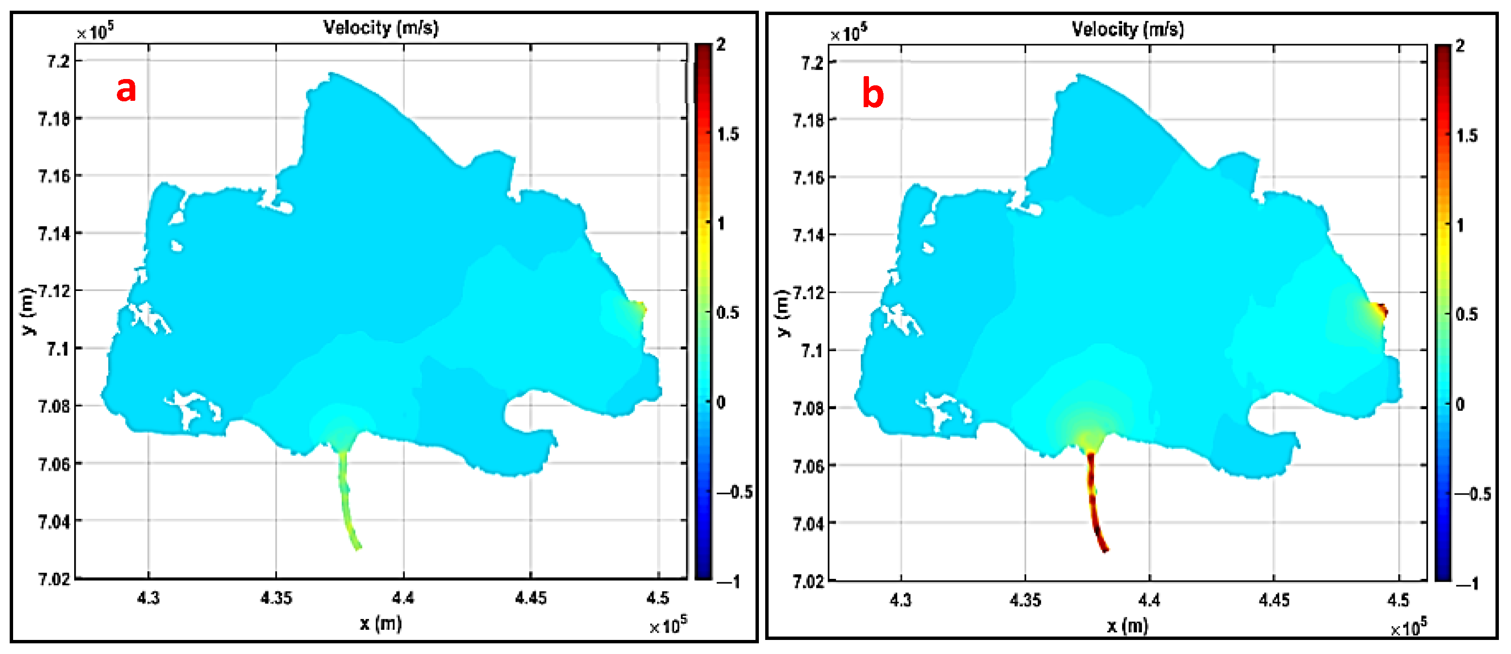
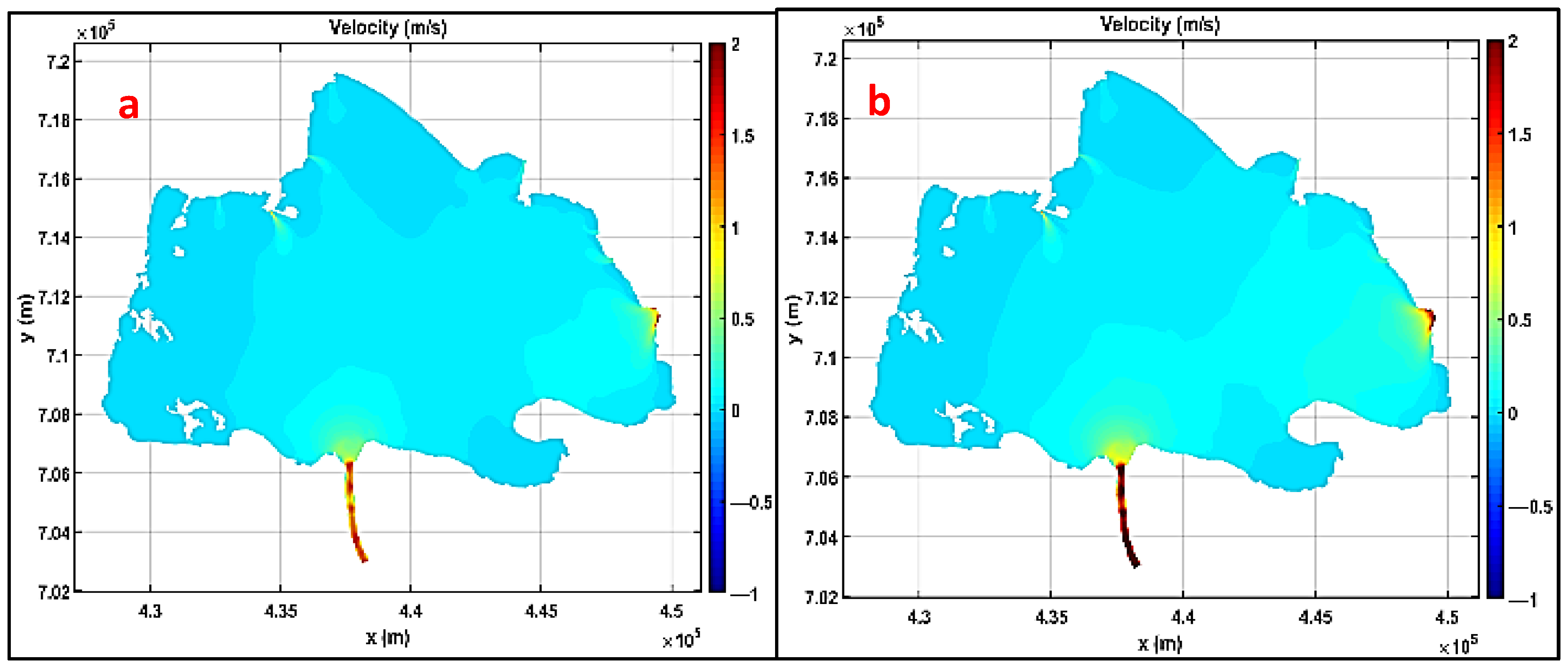
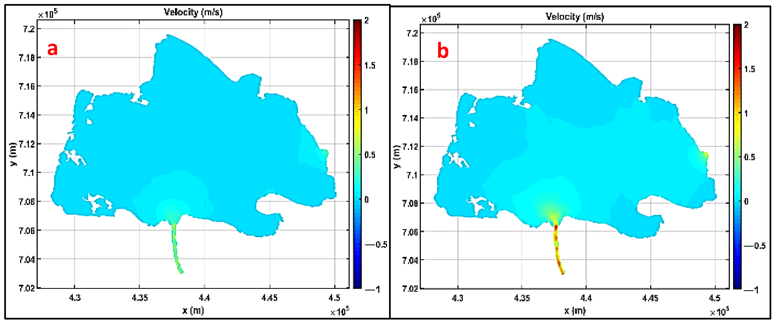
3.3. Velocity Dynamics and Suspended Solids

Residual currents are persistent water movements representing the average flow component, calculated over a period long enough to filter out transient effects such as tides. They result from a balance of forces including pressure gradients, the Coriolis effect due to the Earth’s rotation, density stratification, riverine inputs, and interactions with the lake bottom or riverbed. They play a crucial role in the redistribution of water masses and sediments within estuarine systems. They provide insight into long-term water mass movements driven by forces such as density gradients and tidal asymmetry, which are important for understanding the overall hydrodynamic regime. Residual currents are fundamental for understanding sediment transport and deposition in estuarine and coastal systems. In July, residual velocities are directed southwards (Figure 10a). This southward movement is probably due to the onset of the rainy season, resulting in minimal river input and weak, southward-directed currents due to the prevailing hydrodynamic conditions. In September and November, only particles from the north-east follow the residual current directly into the channel, while particles from the north or north-west circulate around the lake several times before reaching the channel. This behavior indicates that the higher river discharges and intense precipitation that occur during these months result in a complex flow pattern. Water particles from different regions of the lake follow distinct paths before converging on the channel. This complexity signifies stronger hydrodynamic interactions and mixing, influenced by fluvial inputs and precipitation. In March and June, weak currents and tidal influence slow the movement of particles within the lake before they move south.
The tidal influence is more pronounced during these months, resulting in weaker global currents and the significant modulation of particle trajectories due to tidal forces. This suggests that, during the dry season and transition periods, the effects of tides dominate those of fluvial inputs, leading to a distinct pattern of particle movement.
An analysis of the residual current maps shows that there is no significant displacement towards the north, west, or southeast. These areas correspond to zones where fine sediments are present. The lack of movement in these regions indicates that fine sediments are being deposited there due to minimal hydrodynamic disturbance, suggesting that these areas act as sediment deposition zones. This detailed analysis of residual currents and particle movement provides answers to key questions regarding the respective effects of rainfall, tides, and other hydrological factors on sediment transport and hydrodynamics in Nokoué Lake. The analysis shows that, during the rainy season (September to November), high river flows and precipitation significantly influence particle trajectories, resulting in complex flow patterns and increased hydrodynamic mixing. During dry and transitional periods (March and June), however, tidal forces play a dominant role in modulating particle movement, resulting in weaker currents and distinct tidally influenced trajectories. The identifying zones of minimal movement and the presence of fine sediments indicates that certain areas of the lake serve as sediment deposition zones, influenced by prevailing hydrodynamic conditions.
Integrating this information provides an understanding of how various environmental factors, such as precipitation and tides, influence the hydrodynamics and sediment dynamics of Nokoué Lake.
This detailed analysis has enabled us to better understand the specific mechanisms that dominate during each period of the year for Nokoué Lake, whose regime is strongly influenced by the rainy and dry seasons, as well as by the flooding of the Ouémé River. The relative importance of tides compared to river inputs changes radically with the seasons. This detailed understanding is essential for developing management strategies adapted to the lake’s annual variability. It enables us to identify critical periods in terms of sediment transport. This improves our understanding of the lake’s complex hydrological and sedimentary processes and the impact of different drivers.

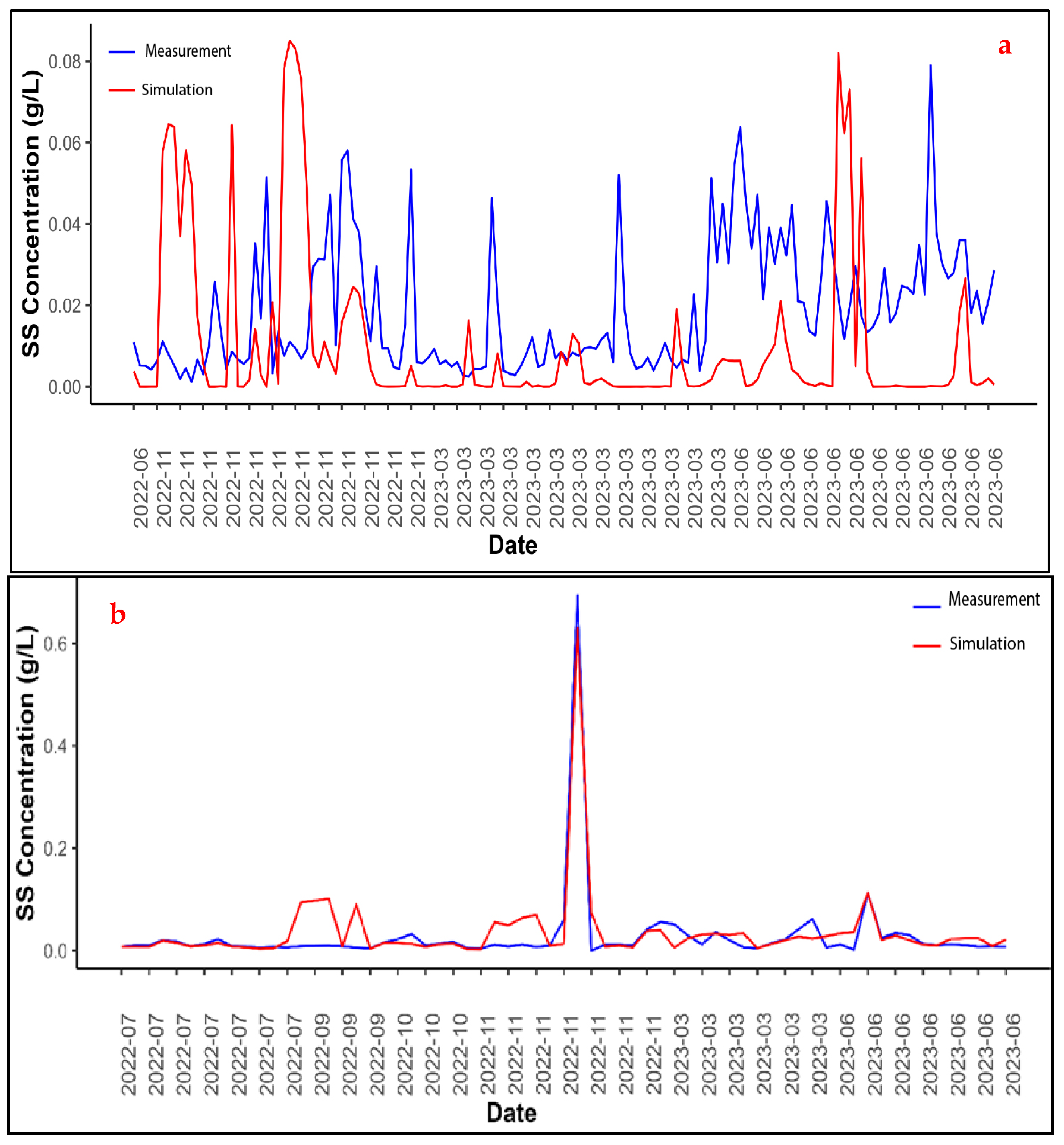
3.4. Validation of the Hydrosedimentary Model

Figure 11 shows how the sediment model was validated using SS concentration data from Nokoué Lake and its boundary conditions. The graphs show a correlation between the measured data and the model predictions.
The calibration results using the R2, NSE, and RMSE efficiency criteria are presented in Table 3. The simulation results for SS concentrations demonstrate a high level of agreement between the observed measurements and the model predictions, particularly in the north-east, south, and south-east regions, as well as in the north-west near the inlets to the Sô River. However, some overestimation was observed, primarily to the south and west of the lake.
The combined approach of field data (in situ measurements) and numerical modelling is a robust and innovative methodology for studying Nokoué Lake. Studies often rely on limited observations or models not validated by substantial datasets. Here, the synergy between the two compensates for a lack of data through modelling and validates the models’ relevance through observations. The result is a more comprehensive and reliable synthesis of the data on the processes occurring in the lake, particularly with regard to SS, which is difficult to sample exhaustively, both space and time. This integration helps to ‘fill the gaps’ in temporal and spatial data series. It also bridges the gap between detailed data and modelling, ensuring reliable predictions.

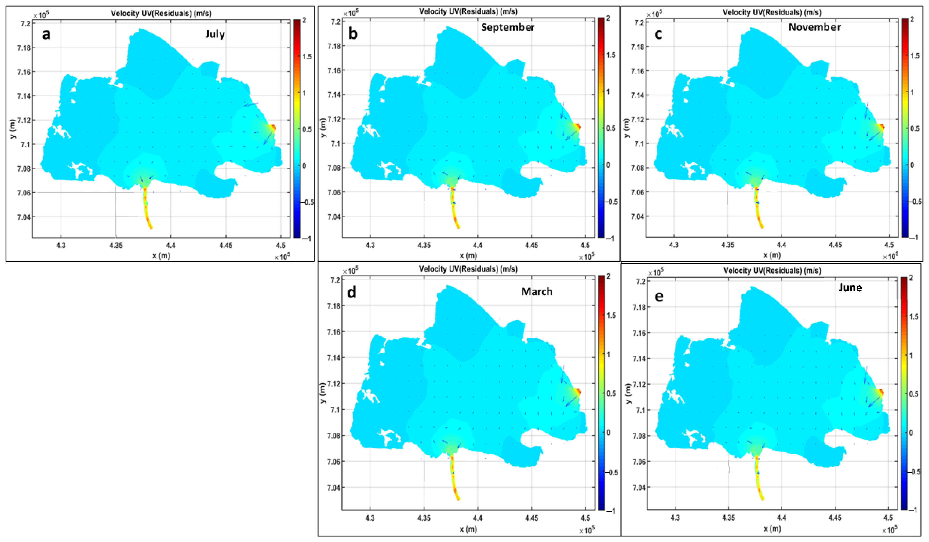
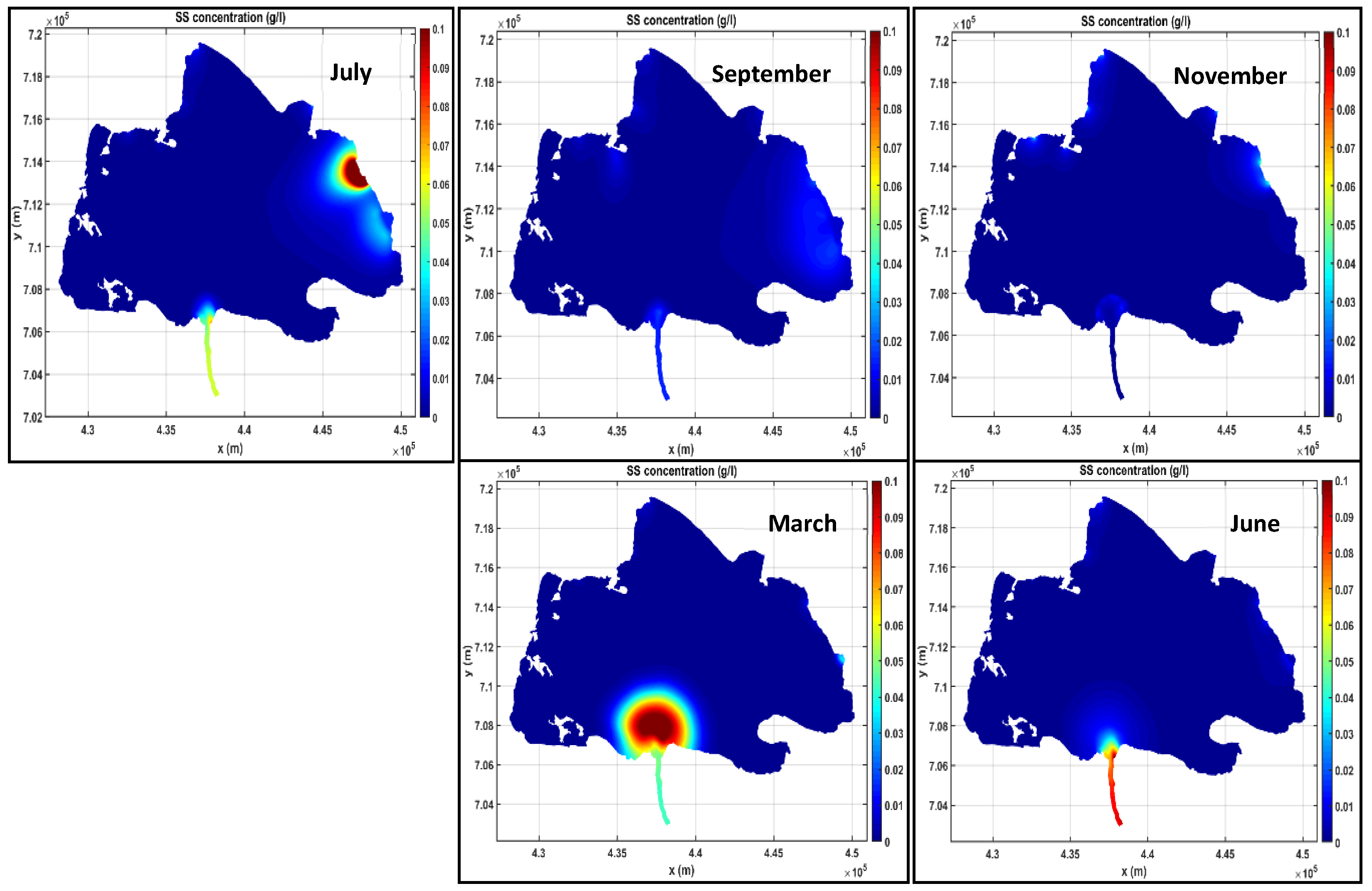
3.5. Distribution of Suspended Solids in the Study Area

An analysis of the spatial and temporal distribution of suspended solids (SS) concentrations obtained through hydrosedimentary modelling using TELEMAC-2D/GAIA reveals significant seasonal variation within Nokoué Lake (see Figure 12). Five maps representing the months of July, September, November, March, and June were examined in order to characterize the sediment fluxes associated with fluvial and anthropogenic inputs.
In July, the center of gravity of the concentrations shifted markedly towards the north-east of the lake, near the confluence with the Ouémé River. SS concentrations also reached high levels of around 0.09 to 0.1 g/L. This pattern reflects the flooding of the Ouémé River during the rainy season and the significant sediment load resulting from the watershed. Moderate concentrations (around 0.05 g/L) were also recorded in the south, reflecting the persistence of dual inputs, both fluvial and anthropogenic.
Despite the continuation of the rainy season in September, TSS concentrations fell sharply across the entire lake. Values did not exceed 0.03 g/L and the lake became noticeably homogeneous. This trend could be due to a generalized dilution phenomenon caused by larger water volumes, the gradual sedimentation of suspended solids or the reduction in external inputs.
At the start of the dry season in November, a slight increase in concentrations is observed in the north-east of the lake, where values reach approximately 0.04 to 0.05 g/L. This localized increase may be due to the residual sediment remobilization in the area affected by the Ouémé River, or to the post-flood accumulation.
In March, at the height of the dry season, the highest concentration of TSS is found in the south of the lake, at the outlet of the Cotonou canal. This area has a core concentration of around 0.1 g/L, which indicates a significant input of suspended solids, most likely from urban, port, and domestic discharges. The southern zone then appears as a major concentration point during periods of low rainfall, probably due to stagnant water and the possible remobilization of sediment deposits.
Finally, in June, which marks the start of the rainy season, a further significant concentration of TSS appears in the same southern area, with maximum values close to 0.1 g/L. The red line along the Cotonou canal indicates intense material flow from urban areas, supported by the first seasonal runoff. The average annual suspended solids flow into the lake from July 2022 to June 2023 is estimated at 17.02 Mt/year.
The study provides dynamic mapping and in-depth spatial and temporal analysis of the distribution of suspended solids (SS) in the lake. This is a significant achievement for Nokoué Lake. Previously, our understanding of SPM distribution was probably limited to isolated measurement points or sporadic observations. Using TELEMAC 2D and GAIA modelling, we can now visualize and quantify how SPMs move, settle, and resuspend depending on hydrological and meteorological conditions such as wind. This has enabled us to identify critical areas of sediment accumulation or erosion, which is fundamental for managing the water quality, navigation, and biodiversity in the lake. Identifying areas of siltation or high turbidity is beneficial for the region. This project directly addresses the objective of understanding and quantifying sediment flux dynamics and improving our understanding of sedimentary mechanisms.

3.6. Model Uncertainty

Considering the limitations of spot measurements and the lack of continuous gauging, a plausible ±30% uncertainty was applied to the reconstructed river discharges. We have established that L is proportional to Q. This simple relationship can be used to, L = Q × C , where C is the mean concentration. This uncertainty propagates directly to the annual sediment flux.
Consequently, the modelled annual suspended solids load of 17 Mt/year is subject to an uncertainty range of
L = 17   M t / y e a r × 1 ± 0.30 = 11.9 , 22.1 M t / y e a r
This uncertainty range highlights the need for more robust hydrological monitoring. Nevertheless, the estimated magnitude is consistent with the expected sediment fluxes in comparable fluvio-lacustrine systems, and does not invalidate the model’s overall order of magnitude.
A second source of uncertainty in this study is the assumption that cohesive sediments have been considered. This decision was based on grain size analyses, which revealed a predominance of fine particles (clay and silt) in most areas of Lake Nokoué. However, it is recognized that some areas, particularly river mouths and areas affected by human activity, may contain coarser materials such as sand and gravel. The lack of explicit modeling of these non-cohesive fractions could lead to an underestimation of local sediment transport dynamics, such as bed load or sand deposition. Future work will adopt a mixed approach, integrating both cohesive and non-cohesive sediments, to better represent the diversity of sedimentological conditions in the lake and enhance the robustness of the results.

4. Discussion

The developed model may present certain uncertainties. Firstly, the model geometry was built using bathymetric data measured in March 2023. Although these data are up to date, their resolution does not fully capture the complexity of the lake bottom morphology. Secondly, anthropogenic activities (such as fishing with fish traps, commonly known as ‘acadja’, and sand dredging) in the area that could influence the zone’s hydrodynamics have not been included in the model. Thirdly, the transport of bottom loads has not been considered, which could result in uncertainty regarding the evolution of the lake bottom. However, this is acceptable, as bottom load contributes only 1–3% to the total load [48,49,50]. Fourthly, to keep the simulations realistic, only the months and periods covered by our data during the high, low, and intermediate seasons were simulated. This may lead to uncertainties in erosion and deposition processes. Nevertheless, this approach is appropriate given that up to 98% of suspended solids in Nokoué Lake is transported during the first rainy season. Finally, the model only considered one type of sediment (cohesive), whereas natural sediments were generally made up of particles of different sizes [39].
Model calibration and validation consisted in comparing simulated water levels with measurements taken over a six-day period. This demonstrated the model’s ability to accurately reproduce fluctuations in water levels and suspended solids (SS) concentrations. The coefficient of determination (R2) was 0.86 and the Nash–Sutcliffe efficiency (NSE) was 0.78 during the calibration stage [22,51]. The correlation between the measured and simulated water levels was strong, with R2 values reaching 0.91 and an NSE of 0.93 for the validation stage [23,24]. However, while the model faithfully reproduces temporal variations, it struggles to capture the amplitude of water levels. This could be due to the temporal differences between the bathymetric survey and the validation period [25].
An analysis of the forces responsible for transporting suspended solids in the lake indicates tidal currents play a role. Wind plays a crucial role in resuspending particles in the lake, leading to increased concentrations of suspended solids [52]. Nevertheless, models indicate that sediment concentrations are lower than measured values, suggesting that additional factors may be at play.
Suspended solids concentrations vary according to the season and the water level. The maximum values are observed in July (0.69 g/L), while the minimum values are observed in March. This is in line with the contributions of the Ouémé River [53]. The Ouémé River contributes up to 94% of suspended solids in July, whereas the Sô and Ouémé Rivers contribute negligibly in March. The analyses also show that tidal activity influences sediment concentrations in March by reducing the number of suspended solids in saltier waters [54]. What distinguishes our study of Nokoué Lake is the integration of these various environmental factors into a unified numerical model adapted to this complex ecosystem.

5. Conclusions

This study examined the hydrodynamics and transport of suspended solids in Nokoué Lake, which is primarily influenced by river inflows and subject to tidal influence via its connection to the Atlantic Ocean. Hydrodynamic modelling using TELEMAC-2D successfully simulated the observed key flow patterns, water levels, and sediment dynamics. The model was calibrated using data from one hydrological year and validated using data from a different time period, thus strengthening the reliability and predictive capacity of the modelling approach. A key strength of this study is the careful selection and calibration of the model parameters controlling sediment transport, namely, the critical erosion shear stress ( τ c e ), erosion rate (M), settling velocity ( W s ), critical shear velocity for deposition ( U * c r ), and the bottom friction coefficient. These parameters are site-specific and reflect the fine, unconsolidated sediment composition of Nokoué Lake. A sensitivity analysis revealed that the critical erosion shear stress ( τ c e ) and the settling velocity ( W s ) have the most significant impact on the model outputs, particularly on the erosion/deposition patterns and the annual sediment flux. These findings emphasize the importance of accurate parameterization, particularly in environments where local sediment characteristics can strongly influence transport dynamics. Although the model performed well under the observed conditions, caution must be exercised when generalizing the calibrated parameters to other periods or systems without proper adjustment. It was found that fluctuating water levels in Nokoué Lake strongly affect sediment processes. High water levels during the rainy season promote erosion and sediment redistribution, whereas lower levels during the dry season promote localized sedimentation. Furthermore, the tide had a greater influence on the flow and suspended solids transport in the Cotonou canal than in the lake itself. During the dry season (e.g., March 2023), the concentration of suspended solids was higher downstream than upstream in the canal due to tidal effects. The opposite trend occurred during the flood season when river inputs dominated. While the model showed a good agreement with the observations, discrepancies remain between the simulated and measured total suspended solids (TSS) due to the potential limitations in the spatial and temporal resolution, the accuracy of the input data, or the unmodelled processes. Nevertheless, this work provides essential insights into sediment dynamics in Nokoué Lake and establishes a robust foundation for future improvements. A further refinement of the sediment parameters through the laboratory or in situ measurements and the inclusion of additional processes, such as cohesive sediment behavior or biogeochemical interactions, could enhance the model’s accuracy in the future. Ultimately, this research supports a better management of Nokoué Lake by providing decision-makers with the tools needed to predict sediment transport under changing hydrological conditions, protect the ecological balance, and ensure the well-being of the communities that depend on the lake.

Author Contributions

T.J.-B.Y., writing—review and editing, writing—original draft, software, methodology, investigation, formal analysis, data curation, and conceptualization; J.T., writing—review and editing, supervision, methodology, investigation, and conceptualization. S.S.G.; editing, supervision, and methodology; G.A.F.A.d., supervision and review. F.K.A., supervision and review. All authors have read and agreed to the published version of the manuscript.

Funding

This work has received financial support from the African Centers of Excellence (ACE) project, which is funded by the World Bank and the French Development Agency (AFD) through the Institute of Research for Development (IRD). The funding number is 6503A1-EAU FF CR0CVN BJ A2L07.

Data Availability Statement

The data are freely available on Zenodo. The DOI is https://doi.org/10.5281/zenodo.15909553.

Acknowledgments

The authors would like to thank the team at the Institute of Research for Development (IRD) in Benin and Marseille. Special thanks go to those who supervised my work on the sediment transport model using the TELEMAC system.

Conflicts of Interest

The authors declare no conflicts of interest.

References

  1. Boukari, O.T.; Dovonou, F.E.; Chouti, W.K.; Dagnon, D.K.; Adjadjihoue, E.; Abou, Y.; Mama, D.; Bawa, L.M. Biomasse planctonique et qualité de l’eau du lac Ahémé au Sud-Ouest du Bénin: Plankton biomass and water quality of Lake Ahémé in south-west of Benin. Int. J. Biol. Chem. Sci. 2022, 16, 1350–1364. [Google Scholar] [CrossRef]
  2. Whitman, W.B.; Coleman, D.C.; Wiebe, W.J. Prokaryotes: The unseen majority. Proc. Natl. Acad. Sci. USA 1998, 95, 6578–6583. [Google Scholar] [CrossRef] [PubMed]
  3. Heise, S.; Förstner, U. Risks from Historical Contaminated Sediments in the Rhine Basin. In The Interactions Between Sediments and Water; Kronvang, B., Faganeli, J., Ogrinc, N., Eds.; Springer: Dordrecht, The Netherlands, 2006; pp. 261–272. [Google Scholar]
  4. Heise, S.; Förstner, U. Risk assessment of contaminated sediments in river basins—Theoretical considerations and pragmatic approach. J. Environ. Monit. 2007, 9, 943. [Google Scholar] [CrossRef] [PubMed]
  5. Grabowski, R.C.; Droppo, I.G.; Wharton, G. Erodibility of cohesive sediment: The importance of sediment properties. Earth-Sci. Rev. 2011, 105, 101–120. [Google Scholar] [CrossRef]
  6. Pérez-Ruzafa, A.; Marcos, C.; Bernal, C.M.; Quintino, V.; Freitas, R.; Rodrigues, A.M.; García-Sánchez, M.; Pérez-Ruzafa, I.M. Cymodocea nodosa vs. Caulerpa prolifera: Causes and consequences of a long term history of interaction in macrophyte meadows in the Mar Menor coastal lagoon (Spain, southwestern Mediterranean). Estuar. Coast. Shelf Sci. 2012, 110, 101–115. [Google Scholar] [CrossRef]
  7. Alongi, D.M. Present state and future of the world’s mangrove forests. Envir. Conserv. 2002, 29, 331–349. [Google Scholar] [CrossRef]
  8. Zhang, C.; Li, M.; Zhao, G.-R.; Lu, W. Harnessing Yeast Peroxisomes and Cytosol Acetyl-CoA for Sesquiterpene α-Humulene Production. J. Agric. Food Chem. 2020, 68, 1382–1389. [Google Scholar] [CrossRef]
  9. Rissanen, K. Crystallography of encapsulated molecules. Chem. Soc. Rev. 2017, 46, 2638–2648. [Google Scholar] [CrossRef]
  10. Ouillon, S. Why and How Do We Study Sediment Transport? Focus on Coastal Zones and Ongoing Methods. Water 2018, 10, 390. [Google Scholar] [CrossRef]
  11. Larsen, S.; Kristiansen, E.; Van Den Tillaar, R. Effects of subjective and objective autoregulation methods for intensity and volume on enhancing maximal strength during resistance-training interventions: A systematic review. PeerJ 2021, 9, e10663. [Google Scholar] [CrossRef]
  12. Siviglia, A.; Crosato, A. Numerical modelling of river morphodynamics: Latest developments and remaining challenges. Adv. Water Resour. 2016, 93, 1–3. [Google Scholar] [CrossRef]
  13. Morel, Y.; Chaigneau, A.; Okpeitcha, V.O.; Stieglitz, T.; Assogba, A.; Duhaut, T.; Rétif, F.; Peugeot, C.; Sohou, Z. Terrestrial or oceanic forcing? Water level variations in coastal lagoons constrained by river inflow and ocean tides. Adv. Water Resour. 2022, 169, 104309. [Google Scholar] [CrossRef]
  14. Djihouessi, M.B.; Aina, M.P. A review of hydrodynamics and water quality of Lake Nokoué: Current state of knowledge and prospects for further research. Reg. Stud. Mar. Sci. 2018, 18, 57–67. [Google Scholar] [CrossRef]
  15. Zandagba, J.; Adandedji, F.M.; Mama, D.; Chabi, A.; Afouda, A. Assessment of the Physico-Chemical Pollution of a Water Body in a Perspective of Integrated Water Resource Management: Case Study of Nokou Lake. J. Environ. Prot. 2016, 7, 656–669. [Google Scholar] [CrossRef]
  16. Chaigneau, A.; Okpeitcha, O.V.; Morel, Y.; Stieglitz, T.; Assogba, A.; Benoist, M.; Allamel, P.; Honfo, J.; Awoulmbang Sakpak, T.D.; Rétif, F.; et al. From seasonal flood pulse to seiche: Multi-frequency water-level fluctuations in a large shallow tropical lagoon (Nokoué Lagoon, Benin). Estuar. Coast. Shelf Sci. 2022, 267, 107767. [Google Scholar] [CrossRef]
  17. Chaigneau, A.; Ouinsou, F.T.; Akodogbo, H.H.; Dobigny, G.; Avocegan, T.T.; Dossou-Sognon, F.U.; Okpeitcha, V.O.; Djihouessi, M.B.; Azémar, F. Physicochemical Drivers of Zooplankton Seasonal Variability in a West African Lagoon (Nokoué Lagoon, Benin). J. Mar. Sci. Eng. 2023, 11, 556. [Google Scholar] [CrossRef]
  18. Okpeitcha, O.V.; Chaigneau, A.; Morel, Y.; Stieglitz, T.; Pomalegni, Y.; Sohou, Z.; Mama, D. Seasonal and interannual variability of salinity in a large West-African lagoon (Nokoué Lagoon, Benin). Estuar. Coast. Shelf Sci. 2022, 264, 107689. [Google Scholar] [CrossRef]
  19. Beighley, J.S.; Hudac, C.M.; Arnett, A.B.; Peterson, J.L.; Gerdts, J.; Wallace, A.S.; Mefford, H.C.; Hoekzema, K.; Turner, T.N.; O’Roak, B.J.; et al. Clinical Phenotypes of Carriers of Mutations in CHD8 or Its Conserved Target Genes. Biol. Psychiatry 2020, 87, 123–131. [Google Scholar] [CrossRef]
  20. Li, L.; Ni, J.; Chang, F.; Yue, Y.; Frolova, N.; Magritsky, D.; Borthwick, A.G.L.; Ciais, P.; Wang, Y.; Zheng, C.; et al. Global trends in water and sediment fluxes of the world’s large rivers. Sci. Bull. 2020, 65, 62–69. [Google Scholar] [CrossRef]
  21. Kryzhanouski, Y. Ronan HERVOUET, Le goût des tyrans. Une ethnographie politique du quotidien en Biélorussie. Lormont: Le Bord de l’Eau, 2020, 282 p. Connexe 2021, 7, 228–231. [Google Scholar] [CrossRef]
  22. Yang, C.; Potts, R.; Shanks, D.R. Enhancing learning and retrieval of new information: A review of the forward testing effect. npj Sci. Learn. 2018, 3, 8. [Google Scholar] [CrossRef]
  23. Gupta, A.; Rodriguez-Hernandez, J.; Slebi-Acevedo, C.J.; Castro-Fresno, D. Improving Porous Asphalt Mixes by Incorporation of Additives; Finnish Transport and Communications Agency Traficom: Helsinki, Finland, 2020. [Google Scholar]
  24. Kumar, T.S.; Rao, N.N.M.; Rawat, R.; Rani, H.S.; Sharma, M.; Sadhu, V.; Sainath, A.V.S. Galactopolymer architectures/functionalized graphene oxide nanocomposites for antimicrobial applications. J. Polym. Res. 2021, 28, 196. [Google Scholar] [CrossRef]
  25. Chen, P.; Shi, W.; Liu, Y.; Cao, X. Slip rate deficit partitioned by fault-fold system on the active Haiyuan fault zone, Northeastern Tibetan Plateau. J. Struct. Geol. 2022, 155, 104516. [Google Scholar] [CrossRef]
  26. Gadel, F.; Texier, H. Distribution and nature of organic matter in recent sediments of Lake Nokoué, Benin (West Africa). Estuar. Coast. Shelf Sci. 1986, 22, 767–784. [Google Scholar] [CrossRef]
  27. Luc, L.B.; Alé, G.; Bertrand, M.; Texier, H.; Yves, B.; René, G. Les Ressources en Eaux Superficielles de la République du Bénin; ORSTOM: Paris, France, 1993. [Google Scholar]
  28. Fink, A.H.; Engel, T.; Ermert, V.; Van Der Linden, R.; Schneidewind, M.; Redl, R.; Afiesimama, E.; Thiaw, W.M.; Yorke, C.; Evans, M.; et al. Mean Climate and Seasonal Cycle. In Meteorology of Tropical West Africa; Parker, D.J., Diop-Kane, M., Eds.; Wiley: Hoboken, NJ, USA, 2017; pp. 1–39. [Google Scholar]
  29. Ahokpossi, Y. Analysis of the rainfall variability and change in the Republic of Benin (West Africa). Hydrol. Sci. J. 2018, 63, 2097–2123. [Google Scholar] [CrossRef]
  30. N’Tcha M’Po, Y.; Lawin, E.; Yao, B.; Oyerinde, G.; Attogouinon, A.; Afouda, A. Decreasing Past and Mid-Century Rainfall Indices over the Ouémé River Basin, Benin (West Africa). Climate 2017, 5, 74. [Google Scholar] [CrossRef]
  31. Guedje, F.K.; Houeto, A.V.V.; Houngninou, E.B.; Fink, A.H.; Knippertz, P. Climatology of coastal wind regimes in Benin. Meteorol. Z. 2019, 28, 23–39. [Google Scholar] [CrossRef]
  32. Biao, E. Assessing the Impacts of Climate Change on River Discharge Dynamics in Oueme River Basin (Benin, West Africa). Hydrology 2017, 4, 47. [Google Scholar] [CrossRef]
  33. Lawin, A.E.; Hounguè, R.; N’Tcha M’Po, Y.; Hounguè, N.R.; Attogouinon, A.; Afouda, A.A. Mid-Century Climate Change Impacts on Ouémé River Discharge at Bonou Outlet (Benin). Hydrology 2019, 6, 72. [Google Scholar] [CrossRef]
  34. Mama, D. Méthodologie et Résultats du Diagnostic de L’eutrophisation du Lac Nokoué (Bénin). Ph.D. Thesis, ÉUniversité de Limoges, Limoges, France, 2010. [Google Scholar]
  35. Djihouessi, M.B.; Djihouessi, M.B.; Aina, M.P. A review of habitat and biodiversity research in Lake Nokoué, Benin Republic: Current state of knowledge and prospects for further research. Ecohydrol. Hydrobiol. 2019, 19, 131–145. [Google Scholar] [CrossRef]
  36. Bajamgnigni Gbambie, A.S.; Steyn, D.G. Sea breezes at Cotonou and their interaction with the West African monsoon: SEA BREEZES AT COTONOU. Int. J. Clim. 2013, 33, 2889–2899. [Google Scholar] [CrossRef]
  37. Hervouet, J. Hydrodynamics of Free Surface Flows: Modelling with the Finite Element Method; Wiley: Hoboken, NJ, USA, 2007. [Google Scholar]
  38. Thiébot, J.; Sedrati, M.; Guillou, S. The Potential of Tidal Energy Production in a Narrow Channel: The Gulf of Morbihan. J. Mar. Sci. Eng. 2024, 12, 479. [Google Scholar] [CrossRef]
  39. Lepesqueur, J.; Hostache, R.; Martínez-Carreras, N.; Montargès-Pelletier, E.; Hissler, C. Sediment transport modelling in riverine environments: On the importance of grain-size distribution, sediment density, and suspended sediment concentrations at the upstream boundary. Hydrol. Earth Syst. Sci. 2019, 23, 3901–3915. [Google Scholar] [CrossRef]
  40. Tassi, P.; Benson, T.; Delinares, M.; Fontaine, J.; Huybrechts, N.; Kopmann, R.; Pavan, S.; Pham, C.-T.; Taccone, F.; Walther, R. GAIA—A unified framework for sediment transport and bed evolution in rivers, coastal seas and transitional waters in the TELEMAC-MASCARET modelling system. Environ. Model. Softw. 2023, 159, 105544. [Google Scholar] [CrossRef]
  41. Krone, R.B. Flume Studies of the Transport of Sediment in Estuarial Shoaling Processes; University of California, Institute of Engineering Research: Pasadena, CA, USA, 1962. [Google Scholar]
  42. Partheniades, E. Erosion and Deposition of Cohesive Soils. J. Hydraul. Div. Proc. Am. Soc. Civ. Eng. 1965, 91, 105–139. [Google Scholar] [CrossRef]
  43. Zanke, U. Mitteilungen des Franzius-Instituts für Wasserbau und Küsteningenieurwesen der Technischen Universität Hannover, chap: Berechnung der Sinkgeschwindigkeiten von Sedimenten; Germany, 1977; pp. 231–245. Available online: https://portal.issn.org/resource/ISSN/0340-0077 (accessed on 19 July 2025).
  44. Thanh, V.Q.; Reyns, J.; Wackerman, C.; Eidam, E.F.; Roelvink, D. Modelling suspended sediment dynamics on the subaqueous delta of the Mekong River. Cont. Shelf Res. 2017, 147, 213–230. [Google Scholar] [CrossRef]
  45. Letrung, T.; Li, Q.; Li, Y.; Vukien, T.; Nguyenthai, Q. Morphology Evolution of Cuadai Estuary, Mekong River, Southern Vietnam. J. Hydrol. Eng. 2013, 18, 1122–1132. [Google Scholar] [CrossRef]
  46. Hung, N.N.; Delgado, J.M.; Güntner, A.; Merz, B.; Bárdossy, A.; Apel, H. Sedimentation in the floodplains of the Mekong Delta, Vietnam Part II: Deposition and erosion. Hydrol. Process. 2014, 28, 3145–3160. [Google Scholar] [CrossRef]
  47. Manh, N.V.; Dung, N.V.; Hung, N.N.; Merz, B.; Apel, H. Large-scale suspended sediment transport and sediment deposition in the Mekong Delta. Hydrol. Earth Syst. Sci. 2014, 18, 3033–3053. [Google Scholar] [CrossRef]
  48. Jordan, C.; Tiede, J.; Lojek, O.; Visscher, J.; Apel, H.; Nguyen, H.Q.; Quang, C.N.X.; Schlurmann, T. Sand mining in the Mekong Delta revisited—Current scales of local sediment deficits. Sci. Rep. 2019, 9, 17823. [Google Scholar] [CrossRef]
  49. Hackney, C.R.; Darby, S.E.; Parsons, D.R.; Leyland, J.; Best, J.L.; Aalto, R.; Nicholas, A.P.; Houseago, R.C. River bank instability from unsustainable sand mining in the lower Mekong River. Nat. Sustain. 2020, 3, 217–225. [Google Scholar] [CrossRef]
  50. Binh, D.V.; Kantoush, S.A.; Ata, R.; Tassi, P.; Nguyen, T.V.; Lepesqueur, J.; Abderrezzak, K.E.K.; Bourban, S.E.; Nguyen, Q.H.; Phuong, D.N.L.; et al. Hydrodynamics, sediment transport, and morphodynamics in the Vietnamese Mekong Delta: Field study and numerical modelling. Geomorphology 2022, 413, 108368. [Google Scholar] [CrossRef]
  51. Tang, T.; Shindell, D.; Faluvegi, G.; Myhre, G.; Olivié, D.; Voulgarakis, A.; Kasoar, M.; Andrews, T.; Boucher, O.; Forster, P.M.; et al. Comparison of Effective Radiative Forcing Calculations Using Multiple Methods, Drivers, and Models. JGR Atmos. 2019, 124, 4382–4394. [Google Scholar] [CrossRef]
  52. Wang, Y. An Empirical Study on the Factors Influencing the Effect of Interactive Video Information Dissemination in Science Popularization. Pop. Sci. Res. 2022, 3, 26–37+106. [Google Scholar]
  53. Banasik, K.; Chojnacki, A.L.; Gebczyk, K.; Grakowski, L. Influence of wind speed on the reliability of low-voltage overhead power lines. In Proceedings of the 2019 Progress in Applied Electrical Engineering (PAEE), Koscielisko, Poland, 17–21 June 2019; IEEE: New York, NY, USA, 2019; pp. 1–5. [Google Scholar]
  54. Ganju, N.K.; Couvillion, B.R.; Defne, Z.; Ackerman, K.V. Development and Application of Landsat-Based Wetland Vegetation Cover and UnVegetated-Vegetated Marsh Ratio (UVVR) for the Conterminous United States. Estuaries Coasts 2022, 45, 1861–1878. [Google Scholar] [CrossRef]
Figure 1. Study area presentation.
Water 17 02209 g001
Figure 2. Map showing the locations of the measurement points on the lake.
Water 17 02209 g002
Figure 3. (a) Bathymetry of Nokoué Lake (bottom level with respect to the mean level); and (b) boundary conditions: Q means that a flow rate is imposed; and H means that a water level is imposed.
Water 17 02209 g003
Figure 4. Comparison between measured and modelled averaged water elevations, averaged over 50 locations in the lake (March 2023).
Water 17 02209 g004
Figure 5. Comparison between measured and modelled averaged water elevations, over 50 locations in the lake for two periods of the year.
Water 17 02209 g005
Figure 6. Comparison between measured and modelled averaged velocity at the boundaries for five periods of the year.
Water 17 02209 g006
Figure 7. Current speed (in m/s) in Nokoué Lake at different time of the tide in July 2022: (a) low-tide; and (b) high-tide period.
Water 17 02209 g007
Figure 8. Current speed (in m/s) in Nokoué Lake at different time of the tide in September 2022: (a) low-tide; and (b) high-tide period.
Water 17 02209 g008
Figure 9. Current speed (in m/s) in Nokoué Lake at different time of the tide in March 2023: (a) low-tide; and (b) high-tide period.
Water 17 02209 g009
Figure 10. Maps of residual currents (in m/s) on the lake at different seasonal periods: (a) July 2022; (b) September 2022; (c) November 2022; (d) March 2023; (e) June 2023.
Water 17 02209 g010
Figure 11. Comparison of the in site and simulated concentration of SS (a) on all the Nokoué Lake and (b) on boundary conditions.
Water 17 02209 g011
Figure 12. Dynamics and distribution of suspended solids concentrations (g/L) on Nokoué Lake.
Water 17 02209 g012
Table 1. Monthly flow rates used as boundary conditions in the hydrodynamic model.
MonthQ1Q2Q3Q4Q5Q6Q7
Jul-2240.10.09.74.06.74.63.7
Sep-22112.137.646.993.477.7137.060.8
Nov-2283.39.85.07.78.53.81.8
Mar-23−31.33.83.26.1−4.23.72.3
Jun-2314.70.2−4.7−3.2−6.76.56.8
Table 2. GAIA model parameters.
ParametersReferences
W s (m/s) U * c r (m/s)M kg/(s.m2)τce (N/m2)
10−4–3·10−48.9·10−3–1.1·10−25·10−6–1·10−40.15–1.5[45]
2.16·10−4–1.85·10−34.5·10−3–5.3·10−35.13·10−6–8·10−60.028–0.044[46]
10−4–1.3·10−34.4·10−3–5·10−3[47]
5·10−5–3.3·10−41.02·10−50.2[44]
Table 3. Model performance assessment.
Water Level VelocityCss
R2NSERMSE (m) R2NSERMSE (m/s)R2NSERMSE (g/L)
Model calibration
0.860.780.26 0.820.770.070.970.960.03
Model validation
0.910.930.08 0.940.950.060.880.870.03
Disclaimer/Publisher’s Note: The statements, opinions and data contained in all publications are solely those of the individual author(s) and contributor(s) and not of MDPI and/or the editor(s). MDPI and/or the editor(s) disclaim responsibility for any injury to people or property resulting from any ideas, methods, instructions or products referred to in the content.

