Article

The Effect of Herbaceous and Shrub Combination with Different Root Configurations on Soil Saturated Hydraulic Conductivity

1
State Key Laboratory of Soil and Water Conservation and Desertification Control, College of Soil and Water Conservation Science and Engineering, Northwest A&F University, No. 26 Xinong Road, Yangling 712100, China
2
College of Desert Control Science and Engineering, Inner Mongolia Agricultural University, Hohhot 010010, China
3
Institute of Water Resources and Hydroelectric Engineering, Xi’an University of Technology, No. 5 South Jinhua Road, Xi’an 710048, China
*
Authors to whom correspondence should be addressed.
Water 2025, 17(15), 2187; https://doi.org/10.3390/w17152187
Submission received: 26 March 2025 / Revised: 25 May 2025 / Accepted: 20 July 2025 / Published: 22 July 2025
(This article belongs to the Special Issue Soil Erosion and Soil and Water Conservation)

Abstract

Information on the effects of differences in root and soil properties on Saturated hydraulic conductivity (Ks) is crucial for estimating rainfall infiltration and evaluating sustainable ecological development. This study selected typical grass shrub composite plots widely distributed in hilly and gully areas of the Loess Plateau: Caragana korshinskii, Caragana korshinskii and Agropyron cristatum (fibrous root), and Caragana korshinskii and Artemisia gmelinii (taproot). Samples were collected at different distances from the base of the shrub (0 cm, 50 cm), with a sampling depth of 0–30 cm. The constant head method is used to measure the Ks. The Ks decreased with increasing soil depth. Due to the influence of shrub growth, there was significant spatial heterogeneity in the distribution of Ks at different positions from the base of the shrub. Compared to the sample location situated 50 cm from the base of the shrub, it was observed that in a single shrub plot, the Ks at the base were higher, while in a grass shrub composite plot, the Ks at the base were lower. Root length density, >0.25 mm aggregates, and organic matter were the main driving factors affecting Ks. The empirical equation established by using principal component analysis to reduce the dimensions of these three factors and calculate the comprehensive score was more accurate than the empirical equation established by previous researchers, who considered only root or soil properties. Root length density and organic matter had significant indirect effects on Ks, reaching 52.87% and 78.19% of the direct effects, respectively. Overall, the composite plot of taproot herbaceous and shrub (Caragana korshinskii and Artemisia gmelinii) had the highest Ks, which was 82.98 cm·d−1. The ability of taproot herbaceous plants to improve Ks was higher than that of fibrous root herbaceous plants. The research results have certain significance in revealing the influence mechanism of the grass shrub composite on Ks.

1. Introduction

Soil hydrological properties have an important role in the redistribution of rainfall [1] Field capacity, saturated water content and saturated hydraulic conductivity (Ks) are considered meaningful soil hydrological parameters [2,3,4]. Saturated hydraulic conductivity (Ks) as one of the important parameters that can reflect the stable infiltration of soil, can better characterize the hydrological change process of the surface and the storage capacity of soil to water in arid and semiarid loess plateau areas and to a certain extent determines the ratio of precipitation infiltrating into the ground and the precipitation flowing from the surface to the river network [2,4]. In arid and semiarid regions, water is the dominant factor affecting vegetation, and determining the infiltration ratio of precipitation can provide a certain basis for rational vegetation allocation under ecological restoration to a certain extent. Therefore, studying Ks after vegetation restoration in arid and semiarid areas is of great significance for estimating rainfall infiltration and evaluating sustainable ecological development [1,5].
The Ks is strongly influenced by vegetation and soil factors [6,7]. The texture, porosity, bulk density, aggregates, organic matter, and other properties of soil can significantly affect the saturated hydraulic conductivity of the soil. Research has shown that Ks often increases with the increase of porosity and >0.25 mm water stable aggregate content, while decreases with the increase of bulk density and clay content [1,5,8,9]. However, the current research results on the influence of soil organic matter on Ks are not consistent. Some scholars have shown that Ks increases with the increase of organic matter [8,10]. However, some studies have also shown that due to the water absorption and expansion effect of organic matter, it may block soil pores and reduce Ks [4,11]. Vegetation mainly affects Ks through its canopy and root system. The vegetation canopy can reduce the energy of raindrops hitting the ground, prevent soil from being compacted by raindrops, and maintain a high Ks [4,12]. The influence of plant roots on Ks mainly depends on their impact on soil structure during the growth process. The growth of roots can not only directly form large pores to increase Ks, but also the interweaving and entanglement structure of plant roots has a certain supporting effect on the soil, which can greatly avoid soil collapsibility, thus maintaining high Ks [4,13,14]. The Loess Plateau is a major area of soil erosion in China, and massive soil erosion poses not only a great danger to the local ecological environment and sustainable agricultural development but also a great threat to the safety of downstream reservoirs and watercourses [15,16]. To prevent water and soil loss and ensure ecological environment security, China has implemented the policy of returning farmland to forests and grasslands since 1999. Since the implementation of this policy, great results have been achieved. Since revegetation, the soil properties of the Loess Plateau have changed dramatically. Most studies have shown that the bulk density, aggregates, organic matter, soil microorganisms, soil porosity and soil fertility on the Loess Plateau have tended to develop well since the implementation of returning farmland to forest and grass [7,10,17,18]. These changes in soil properties have a significant effect on the soil hydrological properties. And the study also found that with different types of vegetation restoration, there are often significant differences in Ks [1,17,19]. However, there is currently a limited study on the impact of vegetation roots on Ks in this region. This makes it unclear which root factors have a significant impact on Ks under different vegetation and soil combinations, which to some extent limits the accuracy of estimating rainfall infiltration in the Loess Plateau [4,20].
As the world’s largest loess accumulation area, studying the Ks of the Loess Plateau after ecological restoration can not only promote the establishment of local ecological hydrological models, but also have certain reference significance for the establishment of hydrological models in the ecological restoration of other loess regions. Grass shrub composite plots, as an important type of plot widely distributed in vegetation restoration on the Loess Plateau, have an extremely important effect in soil and water conservation [21,22]. However, there is still limited research on the influencing factors of soil Ks in grass and shrub composite plots [4,18,23]. Moreover, Yan et al. [24] found that due to the influence of shrub growth, there are differences in herbaceous plant roots at different locations of the shrub. Previous studies indicated that the 50 cm from the base of the shrub was the maximum range where the shrub roots affect the herbaceous roots [21]. However, there is currently limited research on the impact of shrub root distribution on Ks. This leads to a lack of clarity on the mechanism by which grass shrub composite plots affect Ks, and further research is needed.
Therefore, this study selects the loess hilly and gully area with severe erosion on the Loess Plateau. Based on survey research, two mixed communities of Caragana korshinskii and Agropyron cristatum (CK-AC) and Caragana korshinskii and Artemisia gmelinii (CK-AG), which are widely distributed in this area, were selected. Agropyron cristatum is an herbaceous plant with fibrous roots, while Artemisia gmelinii is an herbaceous plant with taproots. Using a single sample plot of Caragana korshinskii (CK) as a control, 0–30 cm of surface soil was collected to explore the changes in Ks and root and soil parameters under different grass-shrub composite plots [21,22,25]. The specific objectives of this study are (1) to explore the variation characteristics of Ks with the sampling plot, sampling location, and depth; (2) to determine the main root and soil parameters that affect Ks; and (3) to estimate Ks using root system and soil parameters.

2. Materials and Methods

2.1. Study Area

The sampling site was located in the Wangmaogou catchment in Suide County, Shaanxi Province (10°20′26″ E–110°22′46″ E, 37°34′13″ N–37°36′03″ N). It experiences a semiarid climate, with a mean annual precipitation of ca.513 mm, with about 73% of the precipitation falling between June and September [21,22]. The soil type in this area is loessial soil, which belongs to silty clay loam. The catchment has an area of 5.97 km2 and belongs to the typical hilly and gully area of the Loess Plateau. In this catchment, the main gully is 3.75 km long and the gully density is 4.31 km·km−2.

2.2. Sample Collection

Table 1 shows the sampling plot, and the sampling was conducted in September 2020. The sampling programme for the study involved the collection of both samples at different sampling positions (at the base of a shrub and 50 cm from the base of a shrub) and samples at different depths (0–5 cm, 5–10 cm, 10–20 cm, 20–30 cm). The age of the shrub was 15 years according to field investigation [21]. During sampling, the aboveground parts were carefully cut back, and the litter was removed from the surface. The sampling orientation was in the downhill direction. A circular cutting ring with a height of 5 cm and a diameter of 5 cm was used for collecting samples for determining the saturated water conductivity and soil bulk density. A special round container with a diameter of 10 cm and a height of 5 cm was used for collecting samples for determining the parameter characteristics of the root system. At the same time, carefully collect undisturbed soil and place it in a box for measuring aggregates, soil particle size, and soil organic matter. Three samples were collected from each plot. There are a total of 72 saturated hydraulic conductivity samples in three plots.

2.3. Sample Determination

(1) Soil sample determination
The method to determine the saturated hydraulic conductivity (Ks) consisted of three steps [4,26]: (1) Undisturbed soil samples were taken outdoors with a cutting ring back to the laboratory and immersed in water for 12 h. The water surface was kept flush with the cutting ring surface during soaking. (2) After reaching 12 h, the cutting ring was removed, and an empty cutting ring was placed on it. The size of the empty ring is exactly the same as that of the soil sample ring. The joint was tightly wound with waterproof tape and then fixed with a rubber ring (Figure 1). (3) Then, the sample was placed on the funnel, and a 500 mL plastic bottle was used to collect samples from under the funnel. The hydraulic head remained at 5 cm throughout the experiment. After stabilizing for 1 h, record the outflow volume every 10 min. In five consecutive measurements, if the error is within 5%, it indicates that the infiltration has stabilized, and the average of these five measurements is taken as the value of water output. If the error exceeds 5% in five consecutive measurements, it indicates that it has not yet stabilized, and the stabilization time should be extended until it stabilizes. Meanwhile, the water temperature was measured at the same time. Three parallel repeated experiments for each sample were conducted when measuring saturated hydraulic conductivity (Ks).
The Saturated hydraulic conductivity (Ks) was calculated as follows:
K t = 10 × Q n × L t n × S × ( h + L )
where, Kt is the Ks at temperature t °C, mm·min−1; Qn is the nth seepage volume, mL; tn is the water connection time, min; S is the soil cross-sectional area, cm2; h is the thickness of the water layer, cm; L is the soil layer thickness, cm.
To facilitate the comparison of Kt values measured at different temperatures, the saturated hydraulic conductivity measured in this experiment was converted into the saturated hydraulic conductivity at 10 °C and can be expressed as follows:
K 10 = K t 0.7 + 0.03 t °
where, K10 is the Ks at a temperature of 10 °C, mm·min−1; t is the temperature of the water at the time of measurement, °C.
The soil bulk density (BD) was determined by the drying method [18]. The soil particle size was measured using a Malvern laser particle size analyzer [27]. The wet sieving method was used for the determination of soil aggregates [28], and the soil organic matter (SOM) was determined by the potassium dichromate [29].
(2) Determination of root sample
Root-soil composite samples collected in a special round container at different depths were placed in a soil sieve (0.25 mm) and rinsed to obtain root samples. The determination of all root system indicators was based on Ma et al. [21], including root mass (RM), root diameter (RD), root surface area (RSA) and root length (RL). The root weight density (RMD, mg·cm−3), root surface area density (RSD, cm2·cm−3) and root length density (RLD, cm·cm−3) were obtained by dividing RM, RL and RSA by the volume of the fixed container, respectively. The volume of the fixed container was 100 cm3.

2.4. Data Analysis

Using one-way ANOVA to analyze the changes of different indicators with sample plots and depths. Using correlation analysis and random forest analysis to determine the main factors affecting Ks. The comprehensive score of the selected indicators was calculated by principal component analysis, and the relationship between the comprehensive score and Ks was simulated by nonlinear regression. The data were analyzed using IBM SPSS Statistics 19.0 and MATLAB R2022a, and the drawing was done using Origin 8.0.

3. Results and Analysis

3.1. The Ks of Different Grass-Shrub Composite Plots

Table 2 represents the Ks at different sampling plots, sampling locations and sampling depths. In all sample plots, the saturated hydraulic conductivity (Ks) showed a decreasing trend as the depth increased. When the sampling location was altered, the Ks of the CK sample plot at the shrub base were found to be slightly higher than those measured at a distance of 50 cm from the shrub base. However, the Ks of the CK-AC sample plot and CK-AG sample plot at a distance of 50 cm from the shrub base were higher than those measured at the shrub base. Overall, the Ks of the grass shrub composite plot were higher than those of the single shrub plot. Compared to the CK plot, the Ks of the CK-AC and CK-AG sample plots increased by 8.07% and 74.36%, respectively. Among the three sample plots, CK-AG had the highest saturated hydraulic conductivity, with a value of 82.98 cm·d−1.

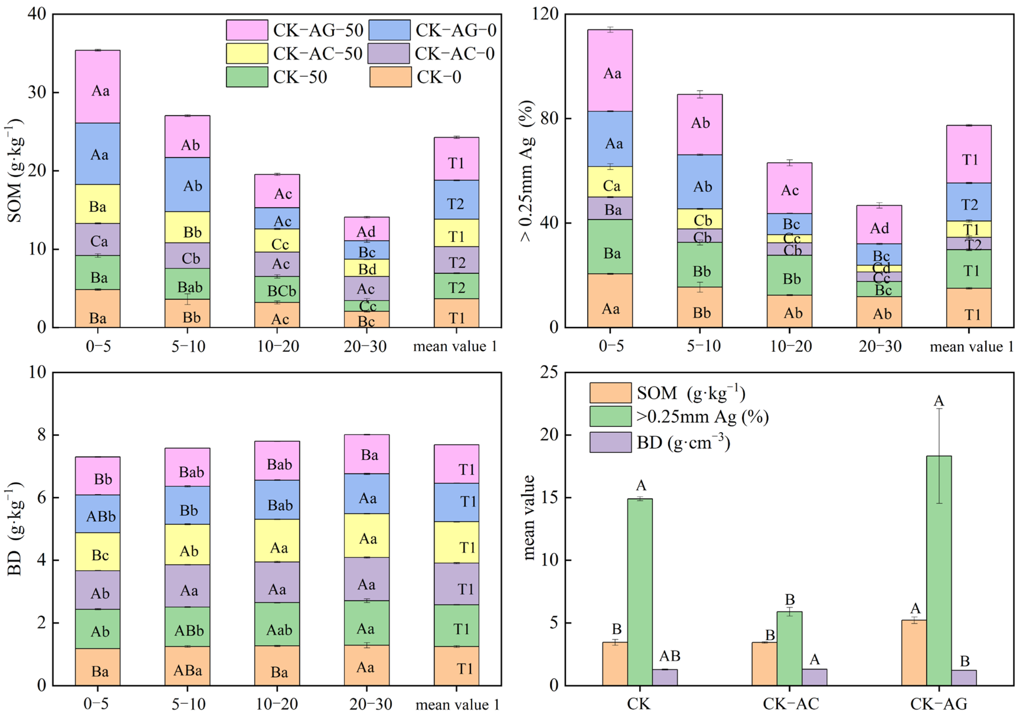
3.2. Root Systems and Soil Indicators in Different Sample Plots

Figure 2, Figure 3 and Figure 4 represent the root systems and soil indicators in different sample plots, sampling locations, and sampling depths. The root systems and soil indicators showed a decreasing trend with increasing depth, except for the soil bulk density (BD), the root diameter (RD), and the soil particle size. To be specific, the soil bulk density (BD) showed an increasing trend with increasing depth, while the root diameter (RD) and the soil particle size changed relatively little. When the sampling location was altered, the SOM, RLD, >0.25 mm aggregates (Ag), and RSD at a distance of 50 cm from the shrub base in composite plots were found to be higher than those measured at the shrub base, while the BD was lower and the RD was finer. The RMD was heavier at the base of shrubs than those measured at the distance of 50 cm from the shrub base in the CK-AG plot, while it showed the opposite trend in the CK-AC plot. In a single shrub plot, the RLD, RMD, RSD, and BD at a distance of 50 cm from the shrub base were higher than those measured at the shrub base, while the values of all other indicators except soil particle size, were lower. There was no significant change in soil particle size with sampling location in all sample plots. When the sample plots were altered, the CK-AG plot exhibited relatively higher levels of SOM, >0.25 mm aggregates (Ag), silt, and RLD among the three sample plots, while the sand, BD, RSD, and RMD of the CK-AC plot were relatively higher among the three sample plots. The CK plot had a relatively higher content of clay and a coarser RD among the three sample plots.

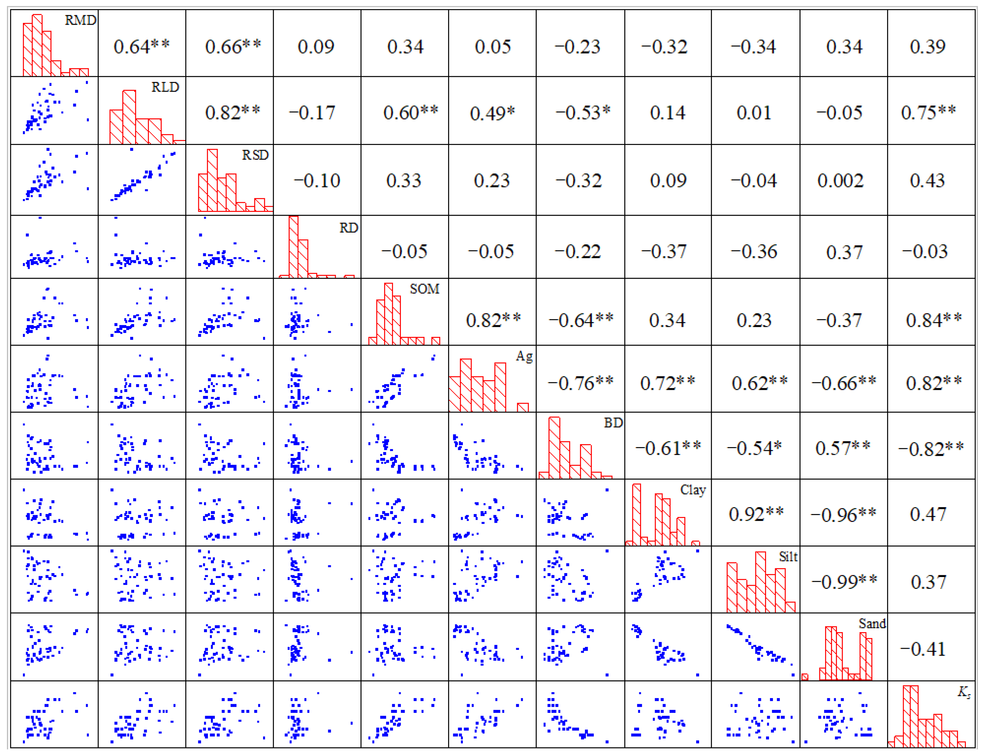
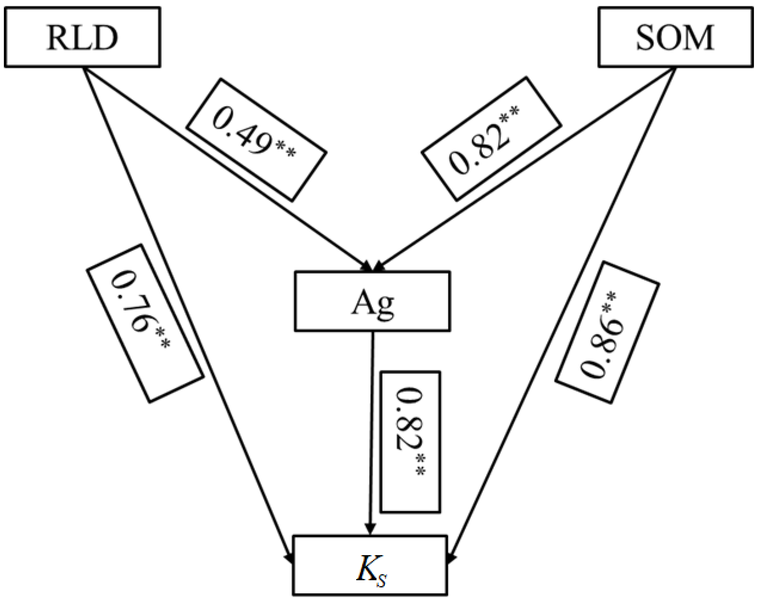
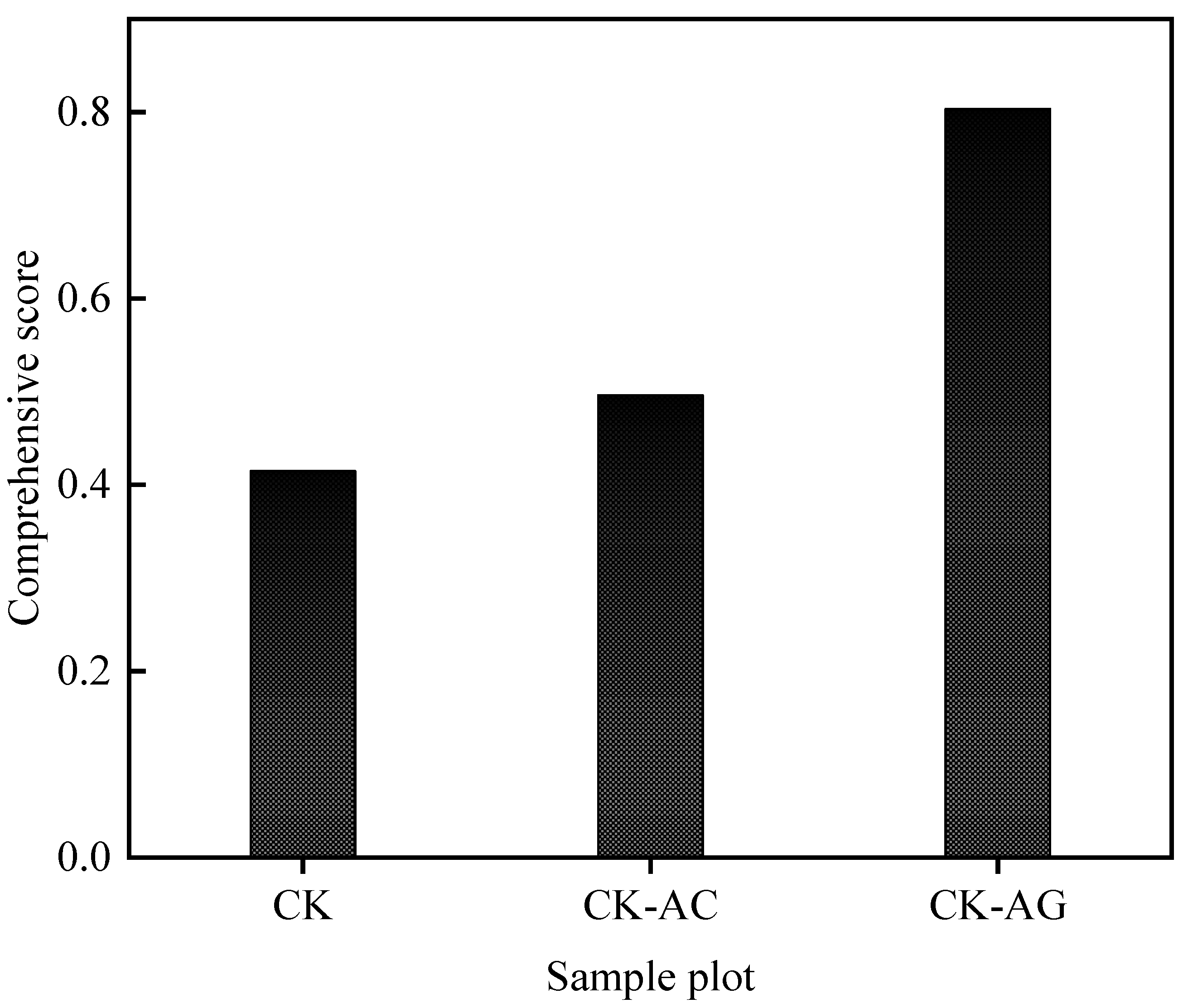
3.3. Importance Analysis of Factors Affecting Ks and Estimation of Ks

To explore the influence of soil properties and root systems on Ks, the study analyzed different factors affecting Ks based on random forest and correlation methods. The analysis results are shown in Table 3 and Figure 5. From Table 3, it can be seen that in the root system indicators, the relative importance order was RLD, RSD, RD, and RMD. In soil indicators, the relative importance order was >0.25 mm aggregates, SOM, BD, Clay, Sand, and Silt. In Figure 5, it can be seen that in the root system indicators, the correlation with Ks was in descending order of RLD, RSD, RMD, and RD. In soil indicators, the correlation with Ks was in descending order of SOM, >0.25 mm aggregates, BD, clay, sand, and silt. To comprehensively consider the effects of soil and root properties on Ks, the RLD in root properties was selected as an indicator for analyzing and simulating Ks by combining the two methods. In soil indicators, it can be seen that >0.25 mm aggregates were of relatively high importance, while SOM exhibited a strong correlation. Due to the fact that aggregates were physical properties of soil, while organic matter was a chemical property of soil. In order to simultaneously consider the influence of soil physical and chemical properties on Ks. In this study, both aggregates and organic matter were selected as indicators for calculating Ks. Overall, the RLD, >0.25 mm aggregates, and SOM were used as indicators for estimating Ks. The simulation results are shown in Table 4. From Table 4, it can be seen that when previous researchers only used root or soil properties to simulate Ks, R2 was only between 0.57 and 0.72. When considering the root system and soil properties comprehensively in this article, the simulation equation (Equation (3)) R2 can reach 0.85, greatly improving the simulation accuracy. To further improve the prediction accuracy of Ks, this study adopts the principal component analysis method (Table 5), fully considering the weight load of each factor, and obtains a comprehensive score based on the weight load of each factor. The R2 of the comprehensive score and the simulation of Ks can reach 0.87 (Equation (4)). Compared to Equation (3), R2 has further improved.
Moreover, it can be seen from the correlation analysis in Figure 5 that there was a strong correlation between RLD, SOM and aggregates. In general, roots and organic matter can improve soil structure by promoting the formation of aggregates and maintaining their stability, thus increasing Ks. To better explore the mechanism of the effects of RLD and SOM on Ks, the study used path analysis. The results are shown in Figure 6, which shows that the path coefficients of the direct effects of RLD and organic matter on Ks were 0.76 and 0.86, respectively, and the path coefficients of the indirect effects were 0.40 and 0.67, respectively. The analysis showed that RLD and organic matter also had a high indirect impact on Ks.

4. Discussion

This experimental study shows that RLD, >0.25 mm aggregates, and SOM are the main driving factors affecting changes in Ks. The relative importance of RLD in the root index may be because RLD can better reflect the interpenetration and twining of roots in soil than can other root indexes. The interpenetration and twining of roots can often reflect the infiltration path that affects soil moisture, which may be the reason why RLD had a greater impact on Ks in the root index [4,13,33]. There are two possible reasons why soil aggregates had a great influence on Ks. First, many studies have shown that soil aggregates have a greater impact on soil bulk density. The bulk density of soil has a significant correlation with soil porosity. As the main path of water infiltration, the amount of soil porosity can directly affect the soil infiltration capacity, which may be the first reason why aggregates have a greater impact on Ks [34,35]. Second, it may be related to the soil characteristics of the Loess Plateau. When encountering water, the soil of the Loess Plateau easily moves, erodes, and even collapses, thus reducing the saturated hydraulic conductivity. The amount of >0.25 mm soil aggregates can reflect the stability of the soil structure [36], which may be the second reason why aggregates have a greater impact on Ks. Soil organic matter, as an important soil cementation material, has an important effect on the formation of aggregates. Additionally, soil organic matter can reflect the fertility of the soil, and the level of soil fertility often has a greater impact on root characteristics, which may be the reason why soil organic matter had a greater impact on Ks [37,38,39].
Due to the well-developed and widespread distribution of shrub roots, there are often differences in the root system and soil properties at different distances from the base of the shrub [12]. In the composite plots of CK-AC and CK-AG, the Ks at 50 cm were higher. This may be related to the distribution of indicators that affect Ks. From the previous analysis, it can be seen that the RLD, the >0.25 mm aggregates, and the SOM have a significant impact on Ks. Therefore, the following analysis will mainly focus on the differences between these three indicators. The results showed that in the composite plots of CK-AC and CK-AG, the SOM, >0.25 mm aggregate and RLD at 50 cm were better overall. As the RLD increases, its influence on soil intertwining is often stronger, and its supporting effect on the porous structure of loess is stronger [13,36,40], which greatly avoids the collapsibility of soil, thus maintaining high soil infiltration. The longer the root system is, the more complex its distribution path in the soil may be. A complex path provides a natural pipeline for water infiltration, thus improving soil infiltration [4,41]. At the same time, from the path analysis in Figure 6, it can also be seen that the root system can also affect the formation of soil aggregates, thereby affecting Ks [33,42]. However, as an important indicator of soil structure, the higher the content of >0.25 mm aggregates, the better the hydraulic conductivity of the soil and the higher the Ks [43,44]. SOM is an important cementation material of soil aggregates. The increase in its content can promote the formation of the Macro-aggregate. Second, soils with high organic matter content often have higher soil fertility [38,39], and the development of plant roots is often better [37]. Therefore, overall, at 50 cm, the RLD, >0.25 mm aggregates, and SOM content are generally better, which may be the reason for its higher Ks.
The order of Ks from big to small was CK-AG, CK-AC and CK. From Figure 2 and Figure 4, it can be seen that the SOM, >0.25 mm aggregate content, and RLD of the sample plot of CK-AG are relatively high, while the SOM, >0.25 mm aggregate content, and RLD are relatively high, and the Ks is often high [4,30,41]. This may be why the high Ks of the CK-AG sample plot. In CK-AC and CK, although the RLD in CK-AC was greater than that in the CK sample plot, the SOM and >0.25 mm aggregates in the CK-AC sample plot were less than those in the CK sample plot. There is an inconsistency in the three indicators. However, in Figure 7, it can be seen that the comprehensive score of principal component analysis of the CK sample plot is lower than that of the CK-AC sample plot. The comprehensive mass fraction of CK was slightly lower than that of CK-AC, which may be the reason that the Ks of its soil were slightly lower than those of CK-AC.
In different sample plots, as the soil depth increases, the overall Ks shows a decreasing trend. This may be because as the soil depth increases, the RLD, >0.25 mm aggregate content, and SOM all show a decreasing trend. The RLD, >0.25 mm aggregate content, and SOM are often positively correlated with Ks [4,41]. Therefore, the decreasing trend of RLD, >0.25 mm aggregate content, and SOM with increasing soil depth may be the reason for the decreasing trend of Ks. At the same time, the study also found that the Ks of CK-AG at 5–20 cm are significantly higher than those of CK-AC. Among them, Agropyron cristatum is a fibrous root herbaceous plant, while Artemisia gmelinii is a taproot herbaceous plant. Research has shown that fibrous root herbaceous plants are mostly distributed on the surface of the soil, while taproot herbaceous plants have deeper roots [21]. The difference in root distribution may be the reason why the CK-AC sample has a high Ks in the surface layer of the soil, while the CK-AG sample has a high Ks in the deep layer of the soil [22]. From the above analysis, it can be seen that when the fibrous root systems of herbs and shrubs are combined, Ks at the surface layer is often higher. When taprooted herbs and shrubs are combined, Ks is often higher in deep layers. Therefore, in the subsequent ecological restoration of arid and semiarid areas, attention should be given to the reasonable combination of herbaceous taproot and fibrous root systems to retain more water and promote ecological restoration.
The measurement of saturated water conductivity is often time-consuming and labor-intensive. Most researchers have simulated saturated water conductivity based on parameters such as soil characteristics and root systems [1,4]. However, previous studies primarily relied on a single parameter (i.e., root length density, soil organic matter and soil aggregates) for simulating saturated water conductivity, as presented in Table 5 [30,31,32]. It is important to note that the accuracy of empirical equations derived from a single parameter for fitting saturated water conductivity tends to be relatively low. Saturated water conductivity results from the combined effects of multiple influencing factors. This study shows that root length density, soil organic matter and >0.25 mm aggregates are the main driving factors affecting changes in Ks. Therefore, the empirical equation for simulating saturated water conductivity comprehensively considers the root length density, soil organic matter and soil aggregates significantly improving the accuracy, with a determination coefficient of 0.85 (see Equation (3) in Table 4). Furthermore, through principal component analysis, the empirical equation for simulating saturated water conductivity (see Equation (4) in Table 4) based on the root length density, soil organic matter and soil aggregates further improves the accuracy, with a determination coefficient of 0.87. The results show that when simulating saturated water conductivity on the slope scale of vegetation restoration, soil properties and root parameters should be comprehensively considered [4,45]. However, due to the number of samples, the applicability of the empirical equation obtained in this study needs further verification. It is worth noting that this study focused on exploring the influence of the impact of root systems and soil properties on the Ks, while ignoring the other influencing factors, such as the vegetation cover and soil microorganisms. Meanwhile, this study did not consider the influence of the interaction of influencing factors on Ks. Therefore, future analyses should comprehensively examine all influencing factors related to Ks and emphasize the development of a robust database for Ks on the Loess Plateau.

5. Conclusions

This study measured the distribution characteristics of Ks at 0–30 cm in different plots, and analyzed the soil and root properties that affect Ks. The results showed that Ks in different plots showed a decreasing trend with increasing soil depth. When the combination of taproot herbaceous plants and shrubs was combined, the Ks at 5–20 cm were higher than those of the combination of fibrous root herbaceous plants and shrubs. When the Ks varied with the sampling location, the trend of variation between the composite plot and the single plot was inconsistent. In a single shrub plot, the Ks at the shrub base was higher, while in a grass shrub composite plot, the Ks was higher at 50 cm from the base of the shrub. Compared to a single shrub plot, the Ks of the grass shrub composite plot were higher. Root length density, >0.25 mm soil aggregates, and soil organic matter were the dominant factors affecting Ks in this experiment. The prediction accuracy of Ks considering both root and soil parameters (R2 = 0.87) was higher than that considering only soil and root parameters (R2 = 0.55–0.72). Path analysis showed that root length density and organic matter have significant indirect effects on Ks, reaching 52.87% and 78.19% of the direct effects, respectively. Overall, among the three plots, the Ks of Caragana korshinskii and Artemisia gmelinii, which were composed of taproot herbaceous and shrub combined, were the highest at 82.98 cm·d−1. The above analysis indicates that there will be differences in the trend of Ks changes between composite plots and single plots. The research results have certain significance in revealing the influence mechanism of the grass shrub composite on Ks.

Author Contributions

Z.Z.: Writing—original draft, Methodology, Investigation, Formal analysis; C.W.: Writing—review and editing, Methodology, Formal analysis; B.M.: Writing—review and editing, Methodology, Funding acquisition; Z.L.: Writing—review and editing, Methodology, Funding acquisition; J.M.: Methodology, Investigation; B.L.: Methodology, Investigation. All authors have read and agreed to the published version of the manuscript.

Funding

This research was supported by grants from the National Natural Science Foundation of China (Grants 42277342, 2022YFF1300800).

Data Availability Statement

The data pertaining to this study are available in the article’s Results section; further inquiries can be directed to the corresponding authors.

Acknowledgments

We would like to thank the editor and the reviewers for their constructive comments and suggestions.

Conflicts of Interest

The authors declare that they have no known competing financial interests or personal relationships that could have appeared to influence the work reported in this paper.

References

  1. Qiu, D.X.; Xu, R.R.; Wu, C.X.; Mu, X.M.; Zhao, G.J.; Gao, P. Vegetation restoration improves soil hydrological properties by regulating soil physicochemical properties in the Loess Plateau, China. J. Hydrol. 2022, 609, 127730. [Google Scholar] [CrossRef]
  2. Zheng, J.Y.; Shao, M.A.; Zhang, X.C. Spatial Variation of Surface Soil Bulk Density and Saturated Hydraulic Conductivity on Slope in Loess Region. J. Soil Water Conserv. 2004, 3, 53–56. [Google Scholar] [CrossRef]
  3. Hardie, M.; Clothier, B.; Bound, S.; Oliver, G.; Close, D. Does biochar influence soil physical properties and soil water availability? Plant Soil 2014, 376, 347–361. [Google Scholar] [CrossRef]
  4. Zhu, P.Z.; Zhang, G.H.; Zhang, B.J. Soil saturated hydraulic conductivity of typical revegetated plants on steep gully slopes of Chinese Loess Plateau. Geoderma 2022, 412, 115717. [Google Scholar] [CrossRef]
  5. Liang, X.F.; Zhao, S.W.; Zhang, Y.; Hua, J. Effects of vegetation rehabilitation on soil saturated hydraulic conductivity in Ziwuling Forest Area. Acta Ecol. Sin. 2009, 29, 636–642. [Google Scholar] [CrossRef]
  6. Sone, J.S.; Oliveira, P.T.S.; Euclides, V.P.B.; Montagner, D.B.; Araujo, A.R.D.; Zamboni, P.A.P.; Vieira, N.O.M.; Carvalho, G.A.; Sobrinho, T.A. Effects of nitrogen fertilisation and stocking rates on soil erosion and water infiltration in a Brazilian Cerrado farm. Agric. Ecosyst. Environ. 2020, 304, 107159. [Google Scholar] [CrossRef]
  7. Wu, W.J.; Chen, G.J.; Meng, T.F.; Li, C.; Feng, H.; Si, B.C.; Siddiue, K.H.M. Effect of different vegetation restoration on soil properties in the semi-arid Loess Plateau of China. Catena 2023, 220, 106630. [Google Scholar] [CrossRef]
  8. Zeng, J.H.; Ma, B.; Guo, Y.X.; Zhang, Z.Y.; Li, G.; Li, Z.B.; Liu, C.G. Effect of biological crust cover on soil saturated hydraulic conductivity under freeze⁃thaw conditions. Acta Ecol. Sin. 2022, 42, 348–358. [Google Scholar] [CrossRef]
  9. Zhang, H.Y.; Liu, Q.J.; Liu, S.T.; Li, J.J.; Geng, J.B.; Wang, L.Z. Key soil properties influencing infiltration capacity after long-term straw incorporation in a wheat (Triticum aestivum L.)–maize (Zea mays L.) rotation system. Agric. Ecosyst. Environ. 2023, 344, 108301. [Google Scholar] [CrossRef]
  10. Dong, L.B.; Fan, J.W.; Li, J.W.; Zhang, Y.; Liu, Y.L.; Wu, J.Z.; Li, A.; Shangguan, Z.P.; Deng, L. Forests have a higher soil C sequestration benefit due to lower C mineralization efficiency: Evidence from the central loess plateau case. Agric. Ecosyst. Environ. 2022, 339, 108144. [Google Scholar] [CrossRef]
  11. Jones, A.; Stolbovoy, V.; Rusco, E.; Gentile, A.R.; Gardi, C.; Marechal, B.; Montanarella, L. Climate change in Europe. 2. Impact on soil. A review. Agron. Sustain. Dev. 2009, 29, 423–432. [Google Scholar] [CrossRef]
  12. Wang, D.; Liu, C.; Yang, Y.; Liu, P.; Hu, W.; Song, H.; Miao, C.; Chen, J.; Yang, Z.; Miao, Y. Clipping decreases plant cover, litter mass, and water infiltration rate in soil across six plant community sites in a semiarid grassland. Sci. Total Environ. 2023, 861, 160692. [Google Scholar] [CrossRef]
  13. Li, Q.; Liu, G.B.; Zhang, Z.; Tuo, D.F.; Bai, R.R.; Qiao, F.F. Relative contribution of root physical enlacing and biochemistrical exudates to soil erosion resistance in the Loess soil. Catena 2017, 153, 61–65. [Google Scholar] [CrossRef]
  14. Liu, Y.; Cui, Z.; Huang, Z.; Manuel, L.V.; Wu, G.L. Influence of soil moisture and plant roots on the soil infiltration capacity at different stages in arid grasslands of China. Catena 2019, 182, 104147. [Google Scholar] [CrossRef]
  15. Huang, Y.S.; Li, P.; An, Q.; Mao, F.J.; Zhai, W.C.; Yu, K.F.; He, Y.L. Long-term Land use/cover changes reducing soil erosion in an ionic rare-earth mineral area of southern China. Land Degrad. Dev. 2021, 32, 4042–4055. [Google Scholar] [CrossRef]
  16. Wang, C.G.; Ma, B.; Wang, Y.X.; Li, Z.B.; Fan, S.B.; Mao, C.Y.; Huo, D. Effects of wheat straw length and coverage under different mulching methods on soil erosion on sloping farmland on the Loess Plateau. J. Soils Sediments 2022, 24, 923–935. [Google Scholar] [CrossRef]
  17. Dou, Y.X.; Yang, Y.; An, S.S.; Zhu, Z.L. Effects of different vegetation restoration measures on soil aggregate stability and erodibility on the Loess Plateau, China. Catena 2020, 185, 104294. [Google Scholar] [CrossRef]
  18. Gu, C.J.; Mu, X.M.; Gao, P.; Zhao, G.J.; Sun, W.Y.; Tatarko, J.; Tan, X.J. Influence of vegetation restoration on soil physical properties in the Loess Plateau, China. J. Soils Sediments 2019, 19, 716–728. [Google Scholar] [CrossRef]
  19. Wu, G.L.; Liu, Y.; Fang, N.F.; Deng, L.; Shi, Z.H. Soil physical properties response to grassland conversion from cropland on the semi-arid area. Ecohydrology 2016, 9, 1471–1479. [Google Scholar] [CrossRef]
  20. Liu, S.Z.; Wang, Y.Q.; An, Z.S.; Sui, H.; Zhang, P.P.; Zhao, Y.L.; Zhou, Z.X.; Xu, L.; Zhou, J.X.; Qi, L.J. Watershed spatial heterogeneity of soil saturated hydraulic conductivity as affected by landscape unit in the critical zone. Catena 2021, 203, 105322. [Google Scholar] [CrossRef]
  21. Ma, J.Y.; Ma, B.; Li, Z.B.; Wang, C.G.; Shang, Y.Z.; Zhang, Z.Y. Determining the mechanism of the root effect on soil detachment under mixed modes of different plant species using flume simulation. Sci. Total Environ. 2023, 858, 159888. [Google Scholar] [CrossRef] [PubMed]
  22. Wang, C.G.; Li, H.R.; Xue, S.B.; Ma, B.; Shang, Y.X.; Li, Z.B. How root and soil properties affect soil detachment capacity in different grass–shrub plots: A flume experiment. Catena 2023, 229, 10721. [Google Scholar] [CrossRef]
  23. Sang, K.X.; Hu, G.L.; Huang, C.; Yang, X.T.; Guo, E.H. Effects of root structure characteristics of 5 plant types on soil infiltration in the Yellow River riparian. Sci. Soil Water Conserv. 2020, 18, 1–8. [Google Scholar] [CrossRef]
  24. Yan, B.L. Shurb-Herbaceous Interactions in a Desert Steppe Under Different Stocking Rate; Inner Mongolia Agricultural University: Hohhot, China, 2019. [Google Scholar]
  25. He, X.J.; Augusto, L.; Goll, D.S.; Ringeval, B.; Wang, Y.P.; Helfenstein, J.L.; Huang, Y.Y.; Yu, K.L.; Wang, Z.Q.; Yang, Y.C.; et al. Global patterns and drivers of soil total phosphorus concentration. Earth Syst. Sci. Data 2021, 13, 5831–5846. [Google Scholar] [CrossRef]
  26. Han, F.P.; Zheng, J.Y.; Li, Z.B.; Zhang, X.C. Effect of PAM on soil physical properties and water distribution. Trans. Chin. Soc. Agric. Eng. 2010, 26, 70–74. [Google Scholar] [CrossRef]
  27. Wang, D.; Fu, B.J.; Chen, L.D.; Zhao, W.W.; Wang, Y.F. Fractal analysis on soil particle size distributions under different land-use types: A case study in the loess hilly areas of the Loess Plateau, China. Acta Ecol. Sin. 2007, 27, 3081–3089. [Google Scholar] [CrossRef]
  28. Zhang, J.J.; Wei, Y.X.; Liu, J.Z.; Yuan, J.C.; Liang, H.; Ren, J.; Cai, H.G. Effects of maize straw and its biochar application on organic and humic carbon in water-stable aggregates of a Mollisol in Northeast China: A five-year field experiment. Soil Tillage Res. 2019, 190, 1–9. [Google Scholar] [CrossRef]
  29. Zhang, M.K.; Walelign, D.B.; Tang, H.J. Effects of Biochar’s Application on Active Organic Carbon Fractions in Soil. J. Soil Water Conserv. 2012, 26, 127–137. [Google Scholar] [CrossRef]
  30. Li, J.X.; He, B.H.; Chen, Y. Root features of typical herb plants for hillslope protection and their effects on soil infiltration. Acta Ecol. Sin. 2013, 33, 1535–1544. [Google Scholar] [CrossRef]
  31. Li, T.C.; Shao, M.A.; Jia, Y.H.; Jia, X.X.; Huang, L.M. Using the X-ray computed tomography method to predict the saturated hydraulic conductivity of the upper root zone in the Loess Plateau in China. Soil Sci. Soc. Am. J. 2018, 82, 1085–1092. [Google Scholar] [CrossRef]
  32. Wang, G.L.; Liu, G.B.; Zhou, S.L. The effect of vegetation restoration on soil stable infiltration rates in small watershed of loess gully region. J. Nat. Resour. 2003, 18, 529–535. [Google Scholar] [CrossRef]
  33. Hao, H.X.; Di, H.Y.; Jiao, X.; Wang, J.G.; Guo, Z.L.; Shi, Z.H. Fine roots benefit soil physical properties key to mitigate soil detachment capacity following the restoration of eroded land. Plant Soil 2020, 446, 487–501. [Google Scholar] [CrossRef]
  34. Elhakeem, M.; Papanicolaou, A.N.T.; Wilson, C.G.; Chang, Y.J.; Burras, L.; Abban, B.; Wysocki, D.A.; Wills, S. Understanding saturated hydraulic conductivity under seasonal changes in climate and land use. Geoderma 2018, 315, 75–87. [Google Scholar] [CrossRef]
  35. Patra, S.; Kaushal, R.; Singh, D.; Kumar, R.; Tossou, A.G.; Durai, J. Surface soil hydraulic conductivity and macro-pore characteristics as affected by four bamboo species in North-Western Himalaya, India. Ecohydrol. Hydrobiol. 2022, 22, 188–196. [Google Scholar] [CrossRef]
  36. Zhu, X.M.; Tian, J.Y. The study Strengthening Anti-Scourability and Penetrability of Soil in Loess Plateau. J. Soil Water Conserv. 1993, 7, 1–10. [Google Scholar] [CrossRef]
  37. Barraclough, P.B. Root growth, macro-nutrient uptake dynamics and soil fertility requirements of a high-yielding winter oilseed rape crop. Plant Soil 1989, 119, 59–70. [Google Scholar] [CrossRef]
  38. Yu, Z.H.; Zhang, J.B.; Zhang, C.Z.; Xin, X.L.; Li, H. The coupling effects of soil organic matter and particle interaction forces on soil aggregate stability. Soil Tillage Res. 2017, 174, 251–260. [Google Scholar] [CrossRef]
  39. Pouladi, N.; Møller, A.B.; Tabatabai, S.; Greve, M.H. Mapping soil organic matter contents at field level with Cubist, Random Forest and kriging. Geoderma 2019, 342, 85–92. [Google Scholar] [CrossRef]
  40. Hao, H.; Qin, J.H.; Sun, Z.X.; Guo, Z.L.; Wang, J.J. Erosion-reducing effects of plant roots during concentrated flow under contrasting textured soils. Catena 2021, 203, 105378. [Google Scholar] [CrossRef]
  41. Hao, H.X.; Wei, Y.J.; Ca, D.N.; Guo, Z.L.; Shi, Z.H. Vegetation restoration and fine roots promote soil infiltrability in heavy-textured soils. Soil Tillage Res. 2020, 198, 104542. [Google Scholar] [CrossRef]
  42. Ma, J.Q.; Wang, W.Q.; Yang, J.; Qin, S.F.; Yang, Y.S.; Sun, C.Y.; Pei, G.; Zeeshan, M.; Liao, H.L.; Liu, L.; et al. Mycorrhizal symbiosis promotes the nutrient content accumulation and affects the root exudates in maize. BMC Plant Biol. 2022, 22, 64. [Google Scholar] [CrossRef]
  43. Aksakal, E.L.; Sari, S.; Angin, I. Effects of vermicompost application on soil aggregation and certain physical properties. Land Degrad. Dev. 2016, 27, 983–995. [Google Scholar] [CrossRef]
  44. Topa, D.; Cara, G.I.; Jităreanu, G. Long term impact of different tillage systems on carbon pools and stocks, soil bulk density, aggregation and nutrients: A field meta-analysis. Catena 2021, 199, 105102. [Google Scholar] [CrossRef]
  45. Wang, B.; Zhang, G.H.; Yang, Y.F.; Li, P.P.; Lu, J.X. Response of soil detachment capacity to plant root and soil properties in typical grasslands on the Loess Plateau. Agric. Ecosyst. Environ. 2018, 266, 68–75. [Google Scholar] [CrossRef]
Figure 1. Device diagram for measuring saturated hydraulic conductivity.
Water 17 02187 g001
Figure 2. Distribution characteristics of soil properties in different sample plots. (Minuscule indicates the difference of different indicators with depth when the sample plot and sampling location are the same. Capital letters indicate differences in the variation of different indicators with sample plots when sampling locations and depths are the same. T1 and T2 represent the differences in the mean values of different indicators at different sampling locations, with T1 > T2. “mean value 1” represents the difference in the mean of different indicators in different sample plots. SOM indicates organic matter. Ag represents aggregates larger than 0.25 mm. BD stands for bulk density. CK-0 represents samples collected from the shrub base of the Caragana korshinskii plot, while CK-50 represents samples collected from a distance of 50 cm from the shrub base of the Caragana korshinskii plot. And so on. “0–5” represents soil samples collected at a depth of 0–5 cm, and so on.)
Water 17 02187 g002
Figure 3. Distribution characteristics of soil particle size in different sample plots. (Minuscule indicates the difference of different indicators with depth when the sample plot and sampling location are the same. Capital letters indicate differences in the variation of different indicators with sample plots when sampling locations and depths are the same. T1 and T2 represent the differences in the mean values of different indicators at different sampling locations, with T1 > T2. “mean value 1” represents the difference in the mean of different indicators in different sample plots. CK-0 represents samples collected from the shrub base of the Caragana korshinskii plot, while CK-50 represents samples collected from a distance of 50 cm from the shrub base of the Caragana korshinskii plot. And so on. “0–5” represents soil samples collected at a depth of 0–5 cm, and so on.)
Water 17 02187 g003
Figure 4. Distribution characteristics of root properties in different plots. (Minuscule indicates the difference of different indicators with depth when the sample plot and sampling location are the same. Capital letters indicate differences in the variation of different indicators with sample plots when sampling locations and depths are the same. T1 and T2 represent the differences in the mean values of different indicators at different sampling locations, with T1 > T2. “mean value 1” represents the difference in the mean of different indicators in different sample plots. CK-0 represents samples collected from the shrub base of the Caragana korshinskii plot, while CK-50 represents samples collected from a distance of 50 cm from the shrub base of the Caragana korshinskii plot. And so on. “0–5” represents soil samples collected at a depth of 0–5 cm, and so on. RMD represents the root weight density. RLD represents root length density. RSD represents the root surface area density. RD represents root diameter.)
Water 17 02187 g004
Figure 5. Binary scatter matrix and correlation coefficient of different indicators. (* represent significant correlation at 0.05 level, ** represent significant correlation at 0.01 level.) (RMD represents the root weight density; RLD represents the root length density; RSD represents root surface area density; RD represents the root diameter; SOM represents organic matter; Ag represents the aggregates larger than 0.25 mm; BD represents the bulk density; Ks represents the Saturated hydraulic conductivity).
Water 17 02187 g005
Figure 6. Path analysis of the influence of root system and soil properties on soil saturated hydraulic conductivity. (The value in the figure shows the degree of influence on saturated hydraulic conductivity. RLD represents the root length density; SOM represents organic matter; Ag represents the aggregates larger than 0.25 mm; Ks represents the Saturated hydraulic conductivity.** represent significant correlation at 0.01 level.)
Water 17 02187 g006
Figure 7. Comprehensive score of root length density, organic matter and aggregate based on principal component analysis. (CK, CK-AC and CK-AG refer to the sample plot with the Caragana korshinskii, the sample plot with the Caragana korshinskii and Agropyron cristatum and the sample plot with the Caragana korshinskii and Artemisia gmelinii, respectively).
Water 17 02187 g007
Table 1. The basic information of the sample site.
Vegetation TypesRoot ArchitectureLocationAspectPlant-Row Spacing
(cm × cm)
Caragana korshinskii (CK)taproot110°22′40″ E,
37°36′25″ N
half-shady slope130 × 120
Caragana korshinskii and Agropyron cristatum (CK-AG)Taproot and fibrous110°22′15″ E,
37°36′40″ N
half-shady slope150 × 120
Caragana korshinskii and Artemisia gmelina (CK-AC)Taproot and fibrous110°22′30″ E,
37°36′32″ N
half-shady slope140 × 110
Table 2. Distribution characteristics of soil saturation hydraulic conductivity (cm·d−1).
Depth (cm)Sampling Plot and Sampling Location
CK-0CK-50CK-AC-0CK-AC-50CK-AG-0CK-AG-50
0–553.62 ± 2.03 AaB66.28 ± 0.29 AaB95.70 ± 5.09 BaAB117.12 ± 4.02 AaA102.76 ± 14.4 AaA105.15 ± 4.07 AaAB
5–1061.53 ± 8.84 AaC61.91 ± 1.53 AaB37.44 ± 4.07 AbB46.04 ± 2.10 AbB85.72 ± 6.07 AaA98.68 ± 9.76 AabA
10–2052.07 ± 3.04 AaC36.61 ± 2.04 BbB34.24 ± 4.07 AbB27.41 ± 2.06 AbC75.12 ± 4.07 AabA78.92 ± 2.16 AbcA
20–3031.20 ± 3.87 AbA17.50 ± 2.10 BcB32.05 ± 1.74 AbA24.21 ± 1.94 BbB47.14 ± 1.44 BbA70.33 ± 2.04 AcA
Mean value149.86 ± 13.43 AB45.57 ± 5.42 AB49.86 ± 10.08 AB53.69 ± 14.52 AB77.69 ± 23.23 AA88.27 ± 16.15 AA
Mean value247.72 ± 4.35T251.77 ± 8.55T282.98 ± 5.02T1
Note: CK, CK-AC and CK-AG respectively refer to Caragana korshinskii, Caragana korshinskii and Agropyron cristatum and Caragana korshinskii and Artemisia gmelinii; ‘0’ and ‘50’ indicate that the sampling locations are at the base of the shrub and at a distance of 50 cm from the base of the shrub, respectively; Mean value1 indicates the mean values of saturated hydraulic conductivity for different depths at the same sampling location; Mean value2 indicates the mean values of saturated hydraulic conductivity for sampling location. The capital letters indicate differences in saturated hydraulic conductivity at different sampling locations for the same plots; The Minuscule letters indicates the difference of saturated hydraulic conductivity with depth; The capitalized slanted letters indicate the difference in soil saturated hydraulic conductivity between different sample plots at the same sampling location and depth; T1 and T2 represent the difference in the mean values of saturated hydraulic conductivity for different sample plots.
Table 3. Ranking of the relative importance of the factors influencing the saturated hydraulic conductivity of the soil.
IndicatorsRMDRLDRSDRDSOMAgBDClaySiltSand
Relative importance0.020.520.150.060.620.790.480.050.020.04
Note: RMD represents the root weight density. RLD represents root length density. RSD represents the root surface area density. RD represents root diameter. SOM indicates organic matter. Ag represents the aggregates larger than 0.25 mm. BD represents the bulk density.
Table 4. Empirical equations for different factors and soil saturation hydraulic conductivity.
EqR2Reference
Previous studiesy = 3.84 × RLD + 23.93 (p < 0.01)0.55[30]
y = 53.65 × InSOM − 9.49 (p < 0.01)0.72[31]
y = 3.04 × Ag + 20.77 (p < 0.01)0.68[32]
This studyy = 11.36 × RLD0.29 × SOM0.30 × Ag0.260.85(Equation (3))
y = 92.71 × x (p < 0.01)0.87(Equation (4))
Note: x is the comprehensive score of the selected indicators after principal component analysis.
Table 5. Factor loadings, Eigenvalue and variance contribution of principal component analysis.
IndexPrincipal 1
Root length density (RLD)0.759
Soil organic matter (SOM)0.92
The aggregates larger than 0.25 mm (Ag)0.895
Eigenvalue2.224
variance contribution74.117%
Disclaimer/Publisher’s Note: The statements, opinions and data contained in all publications are solely those of the individual author(s) and contributor(s) and not of MDPI and/or the editor(s). MDPI and/or the editor(s) disclaim responsibility for any injury to people or property resulting from any ideas, methods, instructions or products referred to in the content.

