Future Residential Water Use and Management Under Climate Change Using Bayesian Neural Networks

Abstract

This study projects future Residential Water Use (RWU) under climate change scenarios using a Bayesian Neural Network (BNN) model that quantifies the relationship between observed temperatures and RWU. Eighteen Global Climate Models (GCMs) under the Shared Socioeconomic Pathway 5–8.5 (SSP5–8.5) scenario were used to assess the uncertainties across these models. The findings indicate that RWU in Republic of Korea (ROK) is closely linked to temperature changes, with significant increases projected in the distant future (F3), especially during summer. Under the SSP5–8.5 scenario, RWU is expected to increase by up to 10.3% by the late 21st century (2081–2100) compared to the historical baseline. The model achieved a root mean square error (RMSE) of 11,400 m³/month, demonstrating reliable predictive performance. Unlike conventional deep learning models, the BNN provides probabilistic forecasts with uncertainty bounds, enhancing its suitability for climate-sensitive resource planning. This study also projects inflows to the Paldang Dam, revealing an overall increase in future water availability. However, winter water security may decline due to decreased inflow and minimal changes in RWU. This study suggests enhancing summer precipitation storage while considering downstream flood risks. Demand management strategies are recommended for addressing future winter water security challenges. This research highlights the importance of projecting RWU under climate change scenarios and emphasizes the need for strategic water resource management in ROK.

1. Introduction

Water demand continues to escalate due to population growth, economic development, and changes in dietary habits [1]. At the same time, increasing temperatures due to climate change are intensifying water consumption, particularly for residential and agricultural uses, which exacerbates stress on freshwater supplies. As a result, water scarcity has become a persistent challenge in many parts of the world. Water scarcity is broadly defined as the failure to meet water demand across all sectors—including environmental needs—due to the impacts of water use on water supply or quality [2,3,4].

A comprehensive analysis of Residential Water Use (RWU) is essential for ensuring the sustainability and resilience of urban water systems [5]. In particular, RWU is known to be sensitive to temperature fluctuations, which are expected to intensify under future climate scenarios [6]. Studies have shown that rising temperatures are correlated with increased RWU in many regions, especially during heatwaves and dry seasons [7,8]. For instance, Balling and Gober [8] and Breyer et al. [9] demonstrated temperature sensitivity in single-family households, while Rathnayaka et al. [10] reported seasonal variation in water use behavior. Nevertheless, capturing the full extent of nonlinear and extreme-case behaviors in the relationships between temperature and RWU remains a challenge in many existing studies.

The purposes of river water intake include domestic, industrial, agricultural, and environmental improvement uses, with exceptionally high agricultural water demand. Agricultural water demand increases sharply during drought conditions, a pattern well-documented in regional assessments, such as climate-driven irrigation studies on the North China Plain [11]. In Republic of Korea (ROK), severe droughts between 2020 and 2023 have reduced river water levels, making river water use difficult. In addition, numerous studies predict an increase in the occurrence and severity of meteorological droughts on the Korean Peninsula in the future [12,13,14]. Recently, there has been a shift from structural approaches (hard path) to nonstructural responses (soft path), such as water use restrictions and water demand management plans.

In Seoul, projected temperature increases are expected to further intensify water demand. Praskievicz and Chang [15] showed a strong correlation between water use and temperature/daylight length using daily and monthly records. According to the Korea Meteorological Administration (KMA), the average annual temperature of Seoul will rise by 1.7–3.1 °C by the mid-21st century and 2.4–6.7 °C by the end of the century under the Shared Socioeconomic Pathways (SSPs) [16]. These projections underscore the urgency of developing climate-sensitive models for urban water planning.

In the late 1980s, as water scarcity became a significant issue, numerous indicators were developed to assess the state of water scarcity globally [1]. Among these, the water use to availability ratio, or the criticality ratio, is another widely used indicator to evaluate water scarcity [17,18]. Most existing water scarcity studies employ water intake variables to represent water use, offering a practical proxy for estimating human pressure on water systems [19]. Globally, anomalies in hydrometeorological variables due to climate change are projected to alter water resources, manifesting as changes in natural precipitation and evapotranspiration patterns [20,21]. However, due to the lack of quantitative intake measurement data worldwide, forecasting changes in future water use is challenging. Consequently, projections of the water use to availability ratio under future climate conditions remain undeveloped.

To overcome these challenges, recent research has turned to deep learning (DL) and machine learning (ML) models, which can effectively capture nonlinear patterns in hydrometeorological data. For example, Guo et al. [22], Mu et al. [23], and Hu et al. [24] implemented LSTM-based models that incorporate temperature, water use history, and calendar effects to forecast short-term demand. Du et al. [25] further improved prediction accuracy by applying principal component analysis (PCA) to LSTM models. However, most prior studies depend heavily on historical water use data, which are often unavailable or unreliable. In contrast, this study adopts a simplified approach using only temperature variables to predict monthly RWU, thereby enhancing model applicability in data-limited contexts.

Thus, this study aims to quantify the relationship between observed meteorological variables and residential water use rates under the assumption that natural climatic conditions influence domestic residential water use in preparation for future droughts. In our previous study, several deep learning models, including CNN, LSTM, XGBoost, and Bayesian Neural Networks (BNNs), were compared to estimate residential water use rates using observed temperature data, and the BNN model was found to offer superior performance due to its ability to quantify predictive uncertainty and improve generalizability [26]. In this study, the BNN was employed to project future domestic water use under Global Circulation Models (GCMs) scenarios. Unlike conventional DL models, the BNN framework provides probabilistic forecasts with predictive uncertainty, making it well-suited for climate-sensitive modeling. In addition, the Bayesian regularization in BNNs mitigates overfitting, contributing to more robust performance in extrapolating future conditions. The total water resources in the corresponding basin were also projected, and the water use to availability ratio was presented by comparing domestic water use with total water resources.

2. Data and Methodology

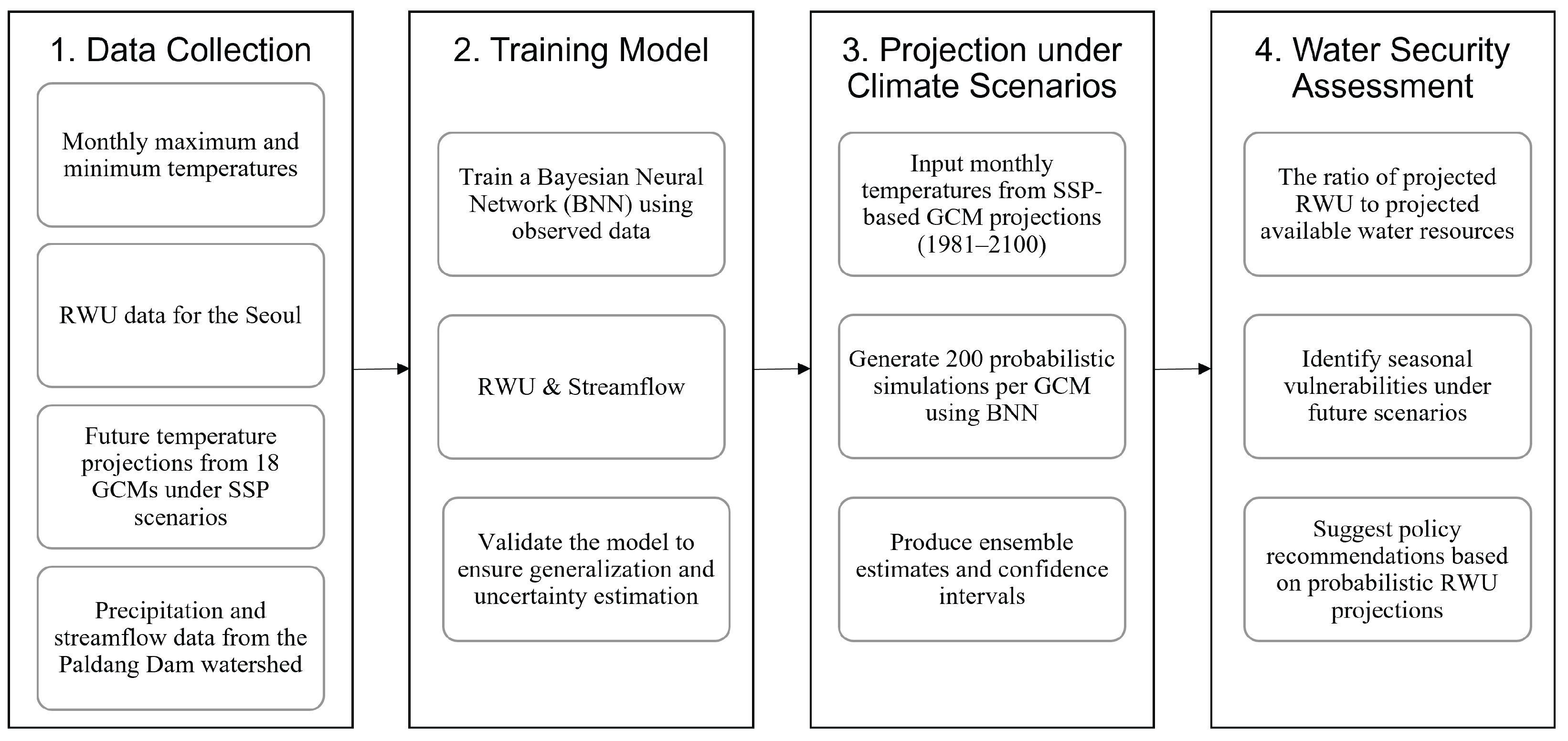
2.1. Study Framework

This study aimed to evaluate future water security by projecting both water availability and Residential Water Use (RWU) under climate change scenarios. As both climatic and anthropogenic factors influence water resource systems, the vulnerability assessment was based on the ratio of future water demand to water availability.

To achieve this, two separate deep learning models were developed. First, a streamflow prediction model was trained using observed hydrometeorological data to simulate future inflows to the Paldang Dam under 18 SSP climate scenarios. Second, a Bayesian Neural Network (BNN) model was developed to project RWU, using historical monthly temperature data as input variables. The BNN was selected for its capacity to incorporate uncertainty in long-term projections.

By comparing the projected RWU with the projected available water resources, this study assesses the seasonal and long-term vulnerability of domestic water use. The workflow of this study is summarized in Figure 1, illustrating the modeling framework and the integration of climate scenario data into the water resource vulnerability assessment.

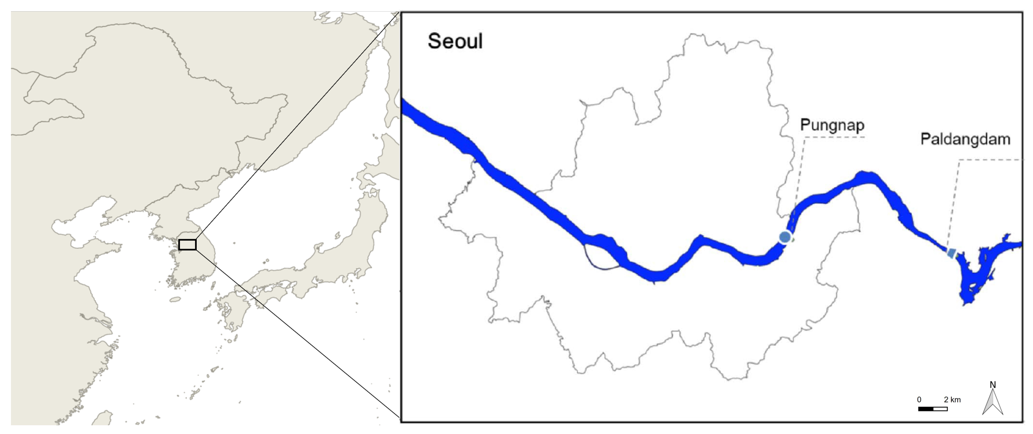
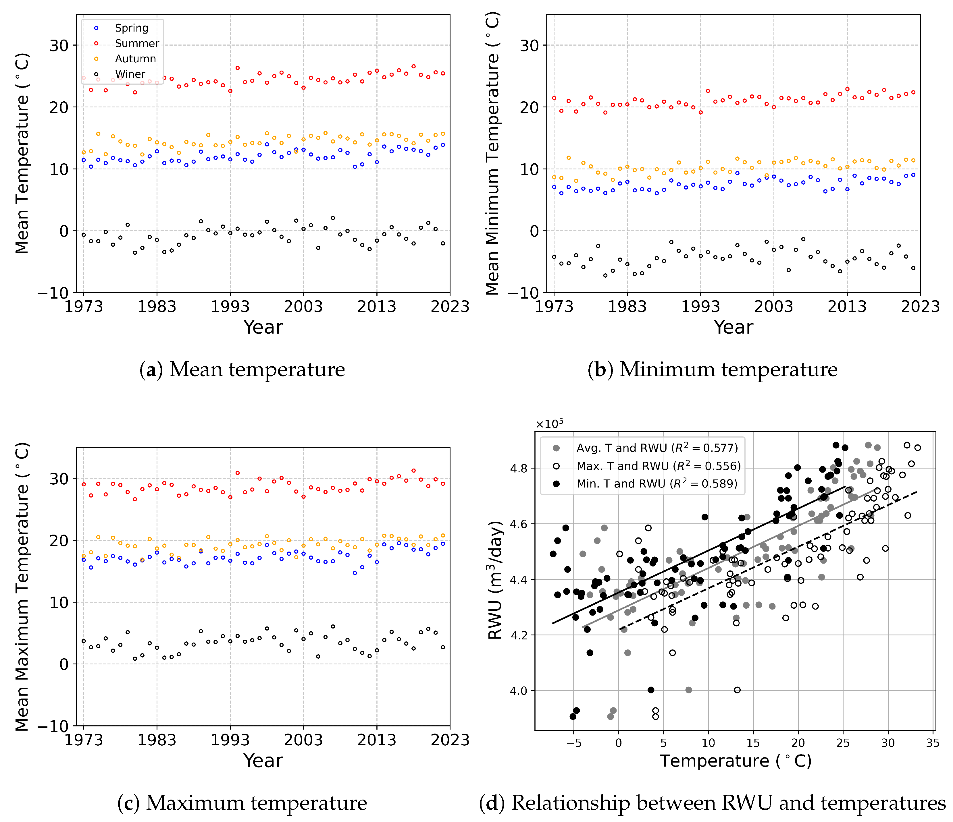
2.2. Study Area and Data

Covering an area of 605.2 km², Seoul accounts for only 0.6% of ROK’s total land area, yet it is home to approximately 9.4 million residents, representing 18.3% of the national population. According to the 2022 Global Power City Index, which evaluates 48 cities worldwide, Seoul ranks as the seventh largest city globally. The city is traversed from east to west by the lower reaches of the Han River. Due to its downstream location, the river has a gentle slope and slow water flow under normal conditions; however, water levels can rise significantly during flood events as runoff from the upper and middle basins flows into the area. The Han River serves as the primary source of domestic water supply for Seoul’s population, with water drawn from the upstream Paldang Dam (Figure 2 [27]).

Figure 3 presents the daily average RWU at the Pungnap water intake plant from 2015 to August 2022. The use was lowest during the winter months (December–February), increased in March, and peaked during the summer months, particularly in July. The daily average RWU in July was 478,580 m³/day (5.5 m³/s). For the other months outside of summer, the RWU remained at relatively similar levels, showing a pattern closely aligned with the variability of ROK’s average temperature. The Pungnap intake exclusively supplies water for municipal use, not for industrial or agricultural purposes. Therefore, the RWU data used in this study represent residential (municipal) water use only.

From 1973 to 2022, the minimum, mean, and maximum temperatures in Seoul were examined. ROK, located in the mid-latitude region of the Korean Peninsula, experiences distinct four seasons, leading to significant seasonal temperature variability. Compared to the average and minimum temperatures, the maximum temperature showed an increasing trend, which was most pronounced during the summer. Notably, the highest recorded temperature was 36.9 °C in 2018, surpassing the previous record of 36.7 °C in 1994. Additionally, the seasonal trends of average, minimum, and maximum temperatures exhibited a 10-year cyclical pattern. This phenomenon is attributed to the periodic rise and fall of the stratospheric temperature in the Pacific atmosphere, which occurs approximately every decade (Figure 4).

Figure 4d presents the correlation between monthly temperatures and RWU from January 2015 to December 2021. Linear regression analyses were conducted separately for mean, minimum, and maximum temperatures against RWU, yielding $R^2$ values of 0.577, 0.589, and 0.556, respectively. These findings indicate a direct relationship, where RWU tends to increase as temperatures rise. Among the three temperature measures, the minimum temperature exhibited the strongest correlation with RWU, approximately 0.77.

Projections of future climate impacts are typically based on climate change scenarios. In this study, climate change scenarios based on SSPs 5–8.5 were collected. Due to significant uncertainty across different climate models, it is essential to quantify these uncertainties and develop detailed regional-scale scenarios for accurate climate representation [12,28]. This study selected 18 GCMs and applied statistical downscaling techniques [29].

Table 1. Details of the Global Circulation Models used in this study.

Institute	GCMs	Resolution	References
Geophysical Fluid Dynamics Laboratory (USA)	GFDL-ESM4	360 × 180	Horowitz et al. [30]
Meteorological Research Institute (Japan)	MRI-ESM2-0	320 × 160	Yukimoto et al. [31]
Centre National de Recherches Meteorologiques (France)	CNRM-CM6-1/CNRM-ESM2-1	24,572 grids (128 lat. circles)	Voldoire et al. [32]; Séférian et al. [33]
Institute Pierre-Simon Laplace (France)	IPSL-CM6A-LR	144 × 143	Boucher et al. [34]
Max Planck Institute for Meteorology (Germany)	MPI-ESM1-2-HR	384 × 192	Schupfner et al. [35]
Met Office Hadley Centre (UK)	UKESM1-0-LL	192 × 144	Dalvi et al. [36]
CSIRO/ARC Centre for Climate System Science (Australia)	ACCESS-CM2	192 × 144	Dix et al. [37]
CSIRO (Australia)	ACCESS-ESM1-5	192 × 145	Ziehn et al. [38]
Canadian Centre for Climate Modelling and Analysis (Canada)	CanESM5	128 × 64	Swart et al. [39]
Institute for Numerical Mathematics (Russia)	INM-CM4-8/INM-CM5-0	180 × 120	Volodin et al. [40]
EC-Earth-Consortium	EC-Earth3	512 × 256	Döscher et al. [41]
Japan JAMSTEC/AORI/NIES/RIKEN	MIROC6/MIROC-ES2L	256 × 128	Shiogama et al. [42]
NorESM Climate Modeling Consortium (Norway)	NorESM2-LM	144 × 96	Seland et al. [43]
NIMS/KMA (Korea)	KACE-1-0-G	192 × 144	Byun et al. [44]

summarizes the GCMs and their details used in this study.

2.3. Bayesian Neural Networks

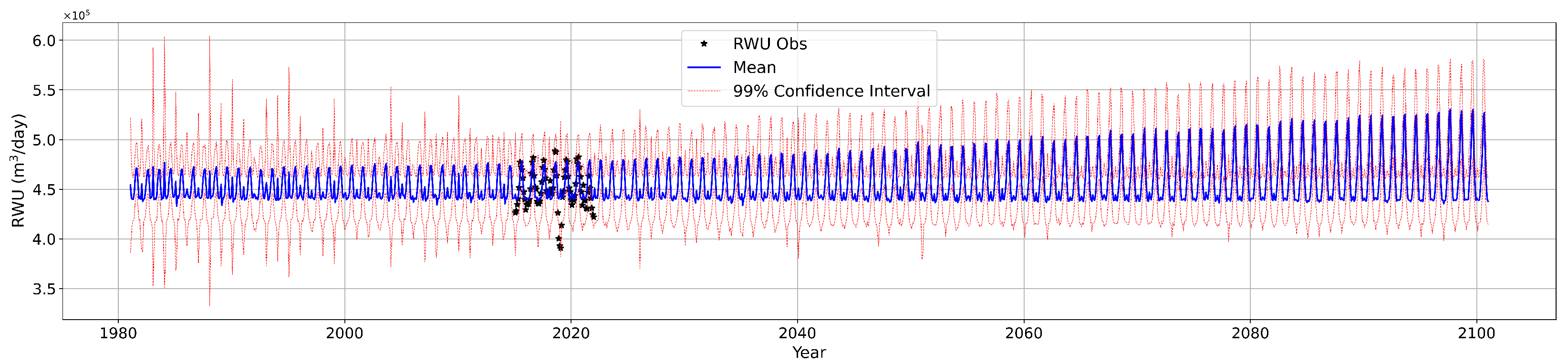
Deep learning is defined as a collection of machine learning algorithms that have evolved from Artificial Neural Network models. While deep learning shares the fundamental characteristic of self-learning with conventional machine learning, it is distinguished by the presence of multiple hidden layers and the ability to autonomously learn not only classifications, but also relevant features without explicit supervision of output values [45,46,47]. Recently, the application of deep learning in the hydrology domain has gained significant attention, as it enables the development and implementation of models capable of capturing complex nonlinear relationships [48,49,50].

Bayesian Neural Networks (BNNs) are a class of stochastic neural networks trained using Bayesian inference [51,52]. BNNs have gained increasing attention due to their ability to provide probabilistic interpretations of model predictions, thereby offering a robust framework for handling uncertainty in deep learning applications. Unlike traditional neural networks, which assign fixed values to model parameters, BNNs estimate the posterior distribution of the parameters through Bayesian inference. This approach enables the quantification of uncertainty in predictions, allowing for more informed decision-making in critical applications.

In a BNN, the network weights are treated as random variables following a probability distribution rather than being fixed scalars. Specifically, each weight, $w_i$, is assumed to follow a Gaussian distribution:

$$p\left(w_i\right)=\mathcal{N}(w_i;{\mu }_i,{\sigma }_i^2)$$

(1)

where ${\mu }_i$ and ${\sigma }_i$ represent the mean and standard deviation of the distribution, respectively. This probabilistic representation enables BNNs to make predictions while also estimating the uncertainty associated with those predictions. The objective of BNN training is to update the prior distribution of weights to obtain their posterior distribution based on observed data. Using Bayes’ theorem, this can be expressed as

$$p\left(\mathbf{w}\right|\mathbf{y},\mathbf{x})={\displaystyle \frac{p\left(\mathbf{y}\right|\mathbf{w},\mathbf{x})·p(\mathbf{w})}{p\left(\mathbf{y}\right|\mathbf{x})}}\propto p\left(\mathbf{y}\right|\mathbf{w},\mathbf{x})·p\left(\mathbf{w}\right)$$

(2)

where $\mathbf{x}$ represents the input vector, $\mathbf{y}$ is the target vector, $p\left(\mathbf{w}\right|\mathbf{y},\mathbf{x})$ denotes the posterior distribution, $p\left(\mathbf{y}\right|\mathbf{w},\mathbf{x})$ is the likelihood function, and $p\left(\mathbf{w}\right)$ is the prior distribution of weights. The term $p\left(\mathbf{y}\right|\mathbf{x})$, known as the evidence, is computationally intractable. Consequently, the variational distribution $q_{\theta }\left(\mathbf{w}\right)$ is introduced to approximate the posterior distribution. The training objective is to minimize the divergence between these distributions using Kullback–Leibler (KL) divergence, which is defined as

$$\underset{\theta }{argmin}KL(q_{\theta }\left(\mathbf{w}\right)\left|\right|p\left(\mathbf{w}\right|\mathbf{y},\mathbf{x}))=\underset{\theta }{argmin}-{\mathbb{E}}_{q_{\theta }\left(\mathbf{w}\right)}\left[log{\displaystyle \frac{p\left(\mathbf{w}\right|\mathbf{y},\mathbf{x})}{q_{\theta }\left(\mathbf{w}\right)}}\right]$$

(3)

To optimize the variational approximation, the relationship between the log-evidence and the ELBO (Evidence Lower Bound) is used:

$$logp\left(\mathbf{y}\right|\mathbf{x})={\mathbb{E}}_{q_{\theta }\left(\mathbf{w}\right)}\left[log{\displaystyle \frac{p\left(\mathbf{y}\right|\mathbf{w},\mathbf{x}\left)p\right(\mathbf{w})}{q_{\theta }\left(\mathbf{w}\right)}}\right]-{\mathbb{E}}_{q_{\theta }\left(\mathbf{w}\right)}\left[log{\displaystyle \frac{p\left(\mathbf{w}\right|\mathbf{y},\mathbf{x})}{q_{\theta }\left(\mathbf{w}\right)}}\right]$$

(4)

where the first term represents ELBO, and the second term corresponds to KL divergence. Since minimizing the KL divergence is equivalent to maximizing the ELBO, the optimization objective can be rewritten as

$$\underset{\theta }{argmin}\mathcal{L}\left(q_{\theta }\right)=\underset{\theta }{argmin}-{\mathbb{E}}_{q_{\theta }}[logp\left(\mathbf{y}\right|\mathbf{w},\mathbf{x})+KL[q_{\theta }\left(\mathbf{w}\right)\left|\right|p\left(\mathbf{w}\right)]]$$

(5)

The ELBO formulation consists of two key components: the likelihood function, which measures model performance; and the KL divergence, which regularizes the network by constraining its weights to follow a prior distribution. This formulation balances model expressiveness while preventing overfitting.

In this study, we employed a customized loss function that incorporates mean squared error (MSE) and Negative Log-Likelihood (NLL), which corresponds to the first term in Equation (5). The loss function is formulated as

$$\mathcal{L}=-(1-\alpha )\sum _{i=1}^N{\mathbb{E}}_{q_{\theta }}[logp\left(y_i\right|f^w\left(x_i\right)]+\alpha \sum _{i=1}^N{(y_i-f^w\left(x_i\right))}^2+KL[q_{\theta }\left(\mathbf{w}\right)\left|\right|p\left(\mathbf{w}\right)]$$

(6)

We demonstrated that the BNN achieves competitive predictive accuracy and the capability to account for uncertainties in RWU predictions [26] and implemented the BNN to model and predict RWU in Seoul, utilizing TensorFlow Probability and TensorFlow to construct a probabilistic deep learning framework. The BNN architecture consisted of five DenseFlipout layers, which utilized variational inference to approximate the posterior distributions of network weights. Each layer employed (1) a mean-field variational posterior, (2) a multivariate normal prior, and (3) KL divergence regularization to control model complexity.

The overall model architecture and training procedures were described in detail in our previous study [26], including the layer configuration, activation functions, and training strategy. The output layer of the model generated parameters for a normal distribution, from which RWU predictions were sampled. To estimate predictive uncertainty, we generated 200 reproductions of RWU by sampling from the predictive distribution for each input. This approach allows for quantifying both the central tendency and the spread (i.e., variance) of the predicted values. For model training, we utilized a combined loss function that balances MSE and NLL, where the weighting coefficient was set to $\alpha =0.1$ with a learning rate of 0.001.

3. Results

3.1. Training the RWU Estimator with the BNN

The relationship between the observed temperature and RWU during the current climate period was quantified using the BNN model. The RWU predictions generated by the models are illustrated in Figure 5a, where blue dots indicate the observed values of the RWU, black stars represent the model’s predicted values, and the colored bands depict the 95% and 99% confidence intervals for the BNN predictions. A black vertical line distinguishes the training set from the validation set, highlighting the model’s performance on previously unseen data.

The model was trained for 30,000 epochs to ensure adequate exposure to the training data. The Equation (6) was used as the loss function to measure the difference between the predicted and actual values. Figure 5b presents the training and validation loss curves for the BNN model, providing insights into their learning dynamics and generalization performance over the training period. The loss curves show a rapid initial decline in training loss, followed by a stabilization phase. This behavior is typical of Bayesian models, which seek to account for uncertainty and converge toward a distribution over weights rather than a single-point estimate. The validation loss closely aligned with the training loss, suggesting that the model effectively generalized to unseen data.

Table 2. Performance metrics for RWU prediction.

Dataset	MAE	RMSE	MAPE	PICP (95%)	PICP (99%)
Train	4660	6760	1.05	0.970	0.985
Validation	9770	11,400	2.19	0.824	1.000
Total	5690	7900	1.28	0.940	0.988

provides a summary of the performance metrics for the model, evaluating their effectiveness in predicting RWU for both the training and validation datasets. The model was assessed using four key metrics: Mean Absolute Error (MAE), which measures the average magnitude of prediction errors; root mean squared error (RMSE), which quantifies overall prediction accuracy by penalizing larger errors; Mean Absolute Percentage Error (MAPE), which expresses prediction error as a percentage of observed values; and Prediction Interval Coverage Probability (PICP), which evaluates the proportion of observed values falling within the model’s predicted uncertainty bounds (Equation (7)).

$$\mathrm{PICP}={\displaystyle \frac{1}{N}}\sum _{i=1}^{N}1\left(y_i\in [{\hat{y}}_i^L,{\hat{y}}_i^U]\right)$$

(7)

where $y_i$ is the observed value at i and N denotes the total number of observations. ${\hat{y}}_i^L$ and ${\hat{y}}_i^U$ represent the lower bound and upper bound of the prediction interval, respectively. $1(·)$ is an indicator function that returns one, if ${\hat{y}}_i^L\le y_i\le {\hat{y}}_i^U$, and zero otherwise.

Examining the MAE and RMSE values, both the training and validation sets exhibited errors within the range of ${10}^3$ to ${10}^4$. Given that the RWU was on the order of ${10}^5$, these error magnitudes indicated that the model achieved sufficiently low prediction errors. The MAPE values further supported this, with the training set showing an average error of 1.05% and the validation set 2.19%, demonstrating reliable predictive performance. Additionally, the PICP results confirmed that the confidence intervals effectively encapsulated the observed values according to their respective probability levels. These findings demonstrated that the BNN model trained in this study successfully reproduced RWU while accounting for uncertainty without signs of overfitting.

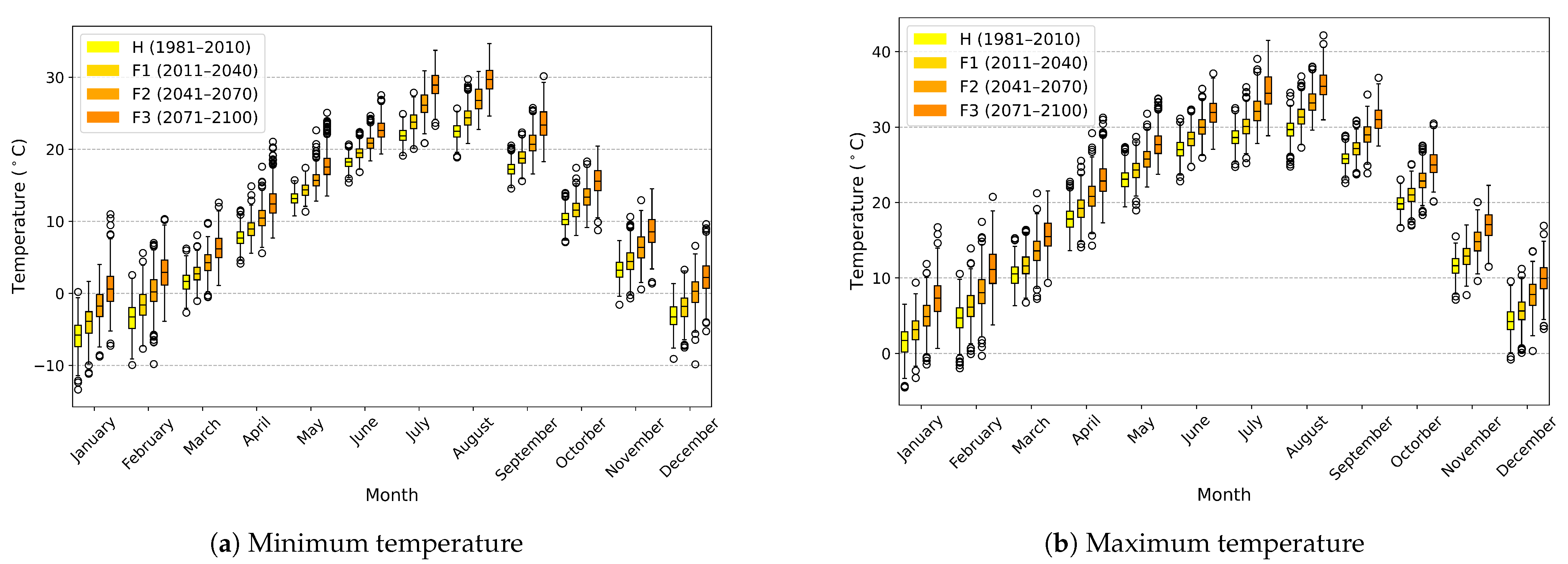
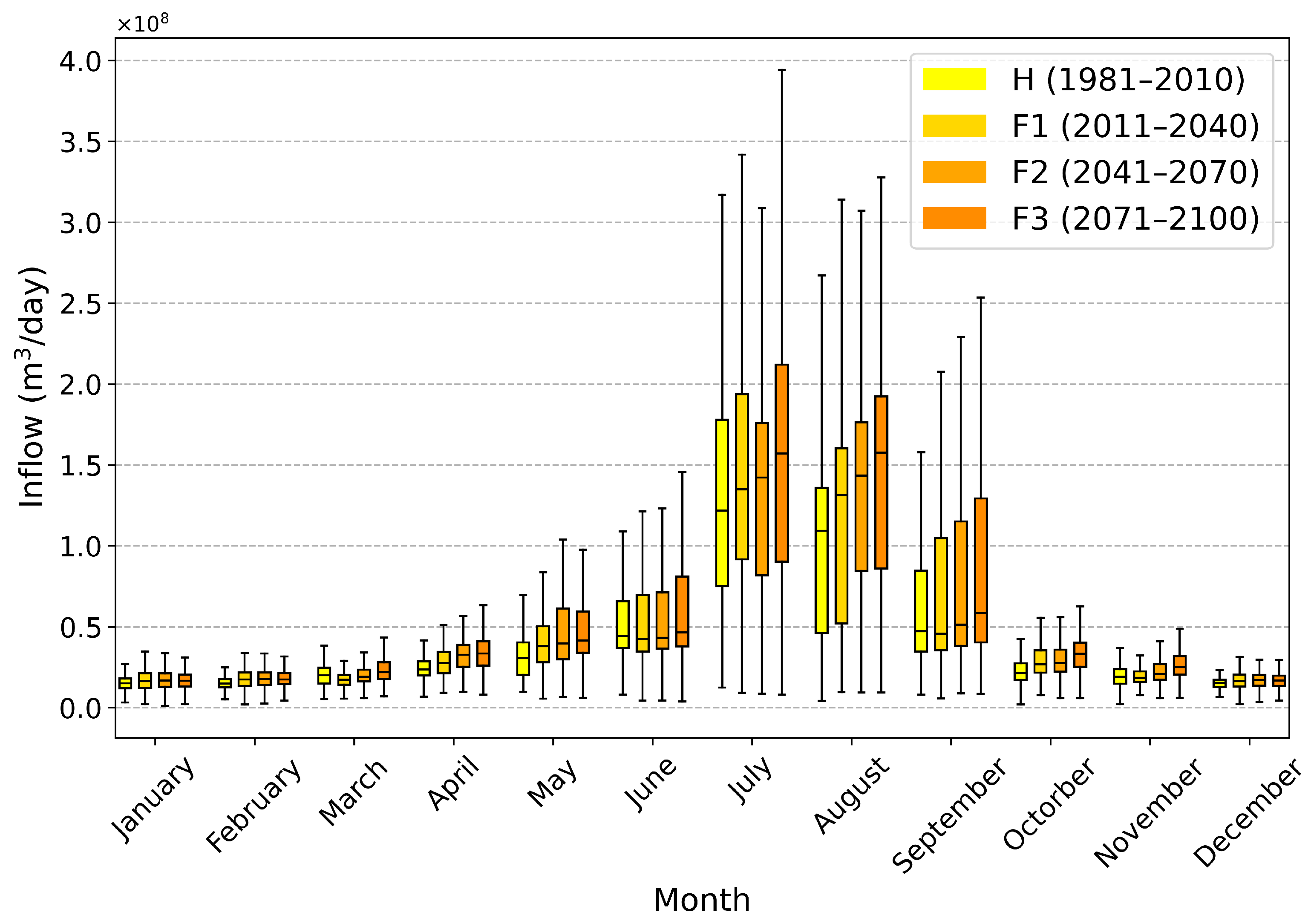
3.2. Future Climate Projections Using CMIP6 GCMs

This study utilized CMIP6 GCM data under the SSP5–8.5 scenario. The SSP scenarios describe global socio-economic trajectories alongside projected greenhouse gas emissions through 2100. These pathways evolve based on future developments across multiple sectors, including socio-economics, technology, energy and industry, policy and governance, and ecosystems. The SSP5–8.5 scenario assumes a high dependency on fossil fuels, leading to urban-centric, unregulated development, resulting in increased environmental vulnerability.

To refine the raw GCM outputs, this study applied spatial downscaling to 18 GCMs (Table 1) and performed systematic bias correction using the quantile mapping (QM) method, calibrated using observational data. QM adjusts the systematic bias in raw GCM simulations to match the target cumulative distribution function (CDF), assuming that the statistical properties of the observed dataset remain stationary over time. The target CDF was developed using 39 years of observational data (1972–2010). For future climate projections, this study analyzed three distinct periods under climate change scenarios, in addition to the historical reference period (H: 1981–2010): (i) early (F1: 2011–2040), (ii) mid-century (F2: 2041–2070), and (iii) late 21st century (F3: 2071–2100).

Figure 6 presents the projected temperature changes under the SSP5–8.5 scenario, comparing future climates to the historical period. The results from 18 GCMs are visualized using box plots, illustrating the monthly temperature distributions for each climate period (H, F1, F2, and F3). The analysis indicated a consistent increase in both average maximum and minimum temperatures over time. Specifically, the average maximum temperature increased from 17.0 °C to 22.6 °C, while the average minimum temperature rose from 8.6 °C to 14.3 °C as the climate progressed into the future.

Additionally, the findings reveal that uncertainty and inter-model variability among GCMs increased over time, particularly in winter months, where temperature variability was more pronounced. This trend was especially evident in the late 21st century (F3), where discrepancies in winter temperature simulations among different GCMs became more apparent. The detailed values for each period are presented in

Table 3. Projected changes in maximum and minimum temperatures under the SSP5–8.5 scenario.

		Jan.	Feb.	Mar.	Apr.	May	Jun.	Jul.	Aug.	Sep.	Oct.	Nov.	Dec.
Max.	Mean (Hist)	1.5	4.7	10.4	17.8	23.0	27.0	28.6	29.6	25.8	19.8	11.6	4.3
	Std (Hist)	1.9	2.1	1.7	1.6	1.3	1.3	1.3	1.4	1.0	1.1	1.4	1.8
	Mean (F1)	3.0	6.2	11.7	19.2	24.3	28.4	30.1	31.4	27.1	21.0	12.9	5.6
	Std (F1)	1.9	2.1	1.7	1.7	1.4	1.4	1.5	1.4	1.2	1.3	1.5	1.8
	Mean (F2)	5.0	8.2	13.5	20.9	25.8	30.0	32.2	33.3	29.0	23.0	14.8	7.7
	Std (F2)	2.1	2.5	1.9	2.0	1.5	1.5	1.9	1.6	1.5	1.5	1.7	2.0
	Mean (F3)	7.4	11.2	15.7	23.0	27.8	31.9	34.9	35.6	31.1	25.2	17.0	10.0
	Std (F3)	2.5	2.9	2.2	2.3	1.8	1.8	2.5	1.9	1.7	1.7	1.9	2.1
Min.	Mean (Hist)	−6.0	−3.4	1.6	7.8	13.2	18.2	21.9	22.5	17.2	10.3	3.2	−3.2
	Std (Hist)	2.2	2.2	1.4	1.2	0.9	0.8	1.0	1.1	1.0	1.1	1.4	1.8
	Mean (F1)	−4.1	−1.6	2.7	8.9	14.3	19.4	23.8	24.4	18.8	11.6	4.5	−1.9
	Std (F1)	2.3	2.1	1.4	1.3	1.0	0.9	1.4	1.4	1.2	1.4	1.7	1.9
	Mean (F2)	−1.8	0.3	4.2	10.5	15.8	20.9	26.3	27.0	20.9	13.4	6.4	0.1
	Std (F2)	2.2	2.3	1.6	1.6	1.2	1.1	1.7	1.8	1.6	1.6	1.9	2.1
	Mean (F3)	0.7	2.9	6.4	12.6	17.8	22.7	28.9	29.6	23.6	15.6	8.7	2.3
	Std (F3)	2.7	2.5	2.1	2.2	1.8	1.5	1.9	1.9	2.2	2.0	2.3	2.4

.

3.3. Residential Water Use Projection Under Climate Change

Using the trained BNN model and the monthly maximum and minimum temperatures projected by 18 GCMs, RWU was predicted for the period 1981–2100. To account for uncertainty, the BNN prediction model was simulated 200 times per GCM, resulting in a total of 3600 RWU projections. Figure 7 presents the RWU projections as a time series over the entire period. The blue line represents the ensemble mean of RWU projections, while the red band illustrates the 99% confidence interval. The observed RWU values are shown as black dots.

The results reveal that the annual maximum RWU values gradually increased over time, whereas the annual minimum RWU values remained relatively unchanged. Additionally, as the predictions extended further from the training period, i.e., as the input temperatures deviated further from the observed period, the uncertainty increased. This reflected the intrinsic characteristics of the BNN model, where uncertainty grew as the model extrapolated beyond the range of its training data.

Using the RWU ensemble time series projections from Figure 7, the monthly variations in RWU under the current and future climate periods were analyzed (Figure 8). In response to overall temperature increases, RWU was projected to increase in future climates compared to the present. However, during the colder months from November to March, when temperatures were lower and RWU is relatively small, little to no change in RWU was observed. The increase in RWU due to climate change was expected to occur primarily between April and October.

Furthermore, winter RWU was projected to be higher in the present than in the future. This reflected the ongoing climate crisis, as evidenced by the frequent occurrence of abnormally high winter temperatures in recent years in ROK. This trend was well captured by multiple climate models, indicating that they effectively represented the current climate conditions.

For colder months, even though temperatures rose due to climate change, they remained within the historically experienced temperature range, leading to reduced uncertainty in RWU projections. However, during the summer months, when RWU peaked, both RWU and its associated uncertainty increased as projections extended further into the future.

To complement the time-series projection results,

Table 4. Monthly RWU statistics for historical and future periods (F1–F3).

		Jan.	Feb.	Mar.	Apr.	May	Jun.	Jul.	Aug.	Sep.	Oct.	Nov.	Dec.
Hist.	Mean (×105)	4.55	4.41	4.41	4.41	4.47	4.62	4.71	4.72	4.57	4.42	4.41	4.43
	Std (×104)	3.13	1.63	0.90	0.86	0.96	1.03	0.99	1.02	0.94	0.87	0.90	1.34
	CV	0.0687	0.0370	0.0204	0.0194	0.0216	0.0224	0.0211	0.0216	0.0206	0.0197	0.0205	0.0303
F1	Mean (×105)	4.47	4.40	4.40	4.42	4.50	4.67	4.79	4.80	4.61	4.43	4.40	4.41
	Std (×104)	1.89	1.16	0.93	0.89	1.00	1.11	1.26	1.23	0.96	0.89	0.90	1.23
	CV	0.0424	0.0264	0.0211	0.0201	0.0222	0.0238	0.0263	0.0257	0.0208	0.0202	0.0204	0.0279
F2	Mean (×105)	4.45	4.40	4.38	4.45	4.56	4.74	4.94	4.97	4.68	4.47	4.39	4.40
	Std (×104)	1.37	1.05	0.91	0.99	1.10	1.26	1.72	1.69	1.07	0.95	0.87	1.10
	CV	0.0309	0.0238	0.0206	0.0223	0.0240	0.0265	0.0348	0.0340	0.0230	0.0213	0.0199	0.0249
F3	Mean (×105)	4.41	4.39	4.39	4.49	4.66	4.84	5.15	5.19	4.78	4.54	4.39	4.39
	Std (×104)	1.31	0.95	0.89	1.16	1.30	1.47	1.95	1.93	1.41	1.08	0.86	0.93
	CV	0.0298	0.0215	0.0203	0.0258	0.0279	0.0304	0.0377	0.0372	0.0294	0.0239	0.0196	0.0213

provides a detailed summary of monthly RWU statistics under historical and future climate scenarios (F1: 2011–2040, F2: 2041–2070, F3: 2071–2100). For each period, the ensemble mean, standard deviation, and coefficient of variation (CV) were calculated across 18 GCMs with 200 stochastic reproductions each.

These statistics quantify both the expected RWU values and their associated uncertainty. Notably, the mean RWU generally increases from the historical period to the far-future scenario, especially from April to October, consistent with seasonal warming patterns. The standard deviation also tends to increase during peak summer months (July–August), reflecting heightened uncertainty in projections under elevated temperature conditions. However, during colder months (e.g., January–March), the uncertainty, reflected by both standard deviation and CV, remains relatively low, as future temperatures fall within the historically observed range.

This table not only supports the trends shown in Figure 7 and Figure 8, but also illustrates how prediction uncertainty evolves over time and across seasons in response to climate change. The scenarios were constructed using monthly maximum and minimum temperature projections from 18 CMIP6 GCMs under the SSP5–8.5 scenario, and simulations were performed for each GCM using the trained BNN model to generate probabilistic RWU forecasts.

3.4. Residential Water Use Projection with Water Resources

The inflow to the Paldang Dam, which supplies water to the Pungnap Intake Facility, was used to determine the available water resources, and the ratio of RWU to available water resources was calculated. To project future changes in available water resources, a BNN model was developed to estimate the inflow to the Paldang Dam using precipitation and maximum and minimum temperatures as input variables. Using this BNN model, the changes in Paldang Dam inflow under future climates were projected relative to the present climate.

The projections indicate that the inflow to Paldang Dam would increase in the future, primarily due to the expected increase in precipitation. Among the seasonal changes, the summer inflows showed the highest rate of increase, but with substantial inter-model variability among the GCMs. In contrast, January inflows, which are typically low, exhibited less inter-model variability compared to the summer months. However, the inflow was projected to decrease in the F3 period compared to F1 and F2 during December, January, and February (DJF) as follows (all values are multiplied by ${10}^7({\mathrm{m}}^3/\mathrm{day})$): (December: 1.803; January: 1.872; February: 2.141), F2 (December: 1.784; January: 1.999; February: 2.146), and F3 (December: 1.754; January: 1.805; February: 2.131) (Figure 9).

Figure 10 represents the projected changes in the ratio of RWU to available water resources, where lower values indicate greater water security. The results show that, in general, this ratio decreased in future periods compared to the present, suggesting that even though future RWU is expected to increase due to rising temperatures, the projected increase in Paldang Dam inflow would be sufficient to meet growing water use.

However, during DJF, the increase in Paldang Dam inflow was relatively modest, and the higher winter temperatures were projected to increase RWU. Consequently, water security was projected to decrease in the F3 period compared to F1 and F2, with the ratios projected as follows (all values are multiplied by ${10}^{-2}$): F1 (December: 2.45; January: 2.39; February: 2.05), F2 (December: 2.47; January: 2.23; February: 2.05), and F3 (December: 2.50; January: 2.44; February: 2.06). This indicates that water security in winter may decline in the late 21st century (F3) due to increased RWU and limited inflow growth.

4. Discussion

Amid the era of the climate crisis, there is growing interest in the impact of climate change on water use, particularly in the domestic and agricultural water use sectors [12,53,54]. Unlike industrial water use, domestic and agricultural water use is closely linked to changes in temperature, making it highly sensitive to climate change. Consequently, water use in these sectors is largely determined by temperature variations.

Sung and Seo [12] demonstrated that Agricultural Water Use (AWU) can be explained by the relationship between precipitation and potential evapotranspiration, with a stronger correlation observed with potential evapotranspiration. In [55], future AWU was projected using potential evapotranspiration derived from temperature projections under future climate scenarios, showing that future AWU would likely increase. Similarly, RWU has shown a strong correlation with temperature [56], and our study also confirmed this significant relationship between RWU and temperature, consistent with this. Based on this strong correlation, the present study quantified the relationship to estimate RWU.

Among the signals of future climate change, one of the most prominent indicators observed in climate change scenarios is the rise in temperatures, and most studies have projected that temperatures in ROK will increase in the future [57]. Moon et al. [57] reported that average temperatures on the Korean Peninsula have risen by approximately 1.5 degrees Celsius over the past century. While this increase may seem moderate, it has already triggered significant changes in weather patterns across ROK. Specifically, the number of extremely hot days during summer is expected to increase, while cold winter days are projected to decrease. The rise in temperatures can lead to changes in potential evapotranspiration, which may subsequently affect the availability of water resources. Gosling and Arnell [58] highlighted that a significant portion of the uncertainty in global projections of water scarcity due to climate change is attributable to uncertainties in South Asia and East Asia.

Despite the strong temperature–RWU relationship identified in this study, several limitations must be acknowledged. The model focused solely on climate variables, specifically monthly maximum and minimum temperatures, as predictors of RWU, while excluding demographic and socioeconomic factors such as population growth, land use changes, or technological advancements. This simplification stems from the observation that Seoul’s population has largely stabilized due to urban saturation, and including uncertain socioeconomic projections could introduce additional layers of uncertainty into the forecasts. Therefore, a parsimonious modeling approach was adopted to isolate the climate signal and minimize confounding effects.

To compensate for this structural simplicity, we implemented an ensemble-based Bayesian Neural Network (BNN) approach which explicitly quantified predictive uncertainty. The probabilistic output of the BNN enabled the generation of prediction intervals rather than point estimates, offering critical insight for water resource management under climate uncertainty. This allows for decision-makers to assess risk and prepare for a range of plausible future outcomes, particularly in regions where temperature-sensitive water use is dominant.

Our study also detected changes in water security over certain periods, revealing a particular vulnerability during winter. Water resource crises [58] require a comprehensive assessment that considers not only the changes in natural river flow due to climate change, but also the impacts of anthropogenic water use. This is because climate change not only alters the natural hydrological cycle, but also influences human water consumption patterns.

However, there is a lack of data on anthropogenic water use, making it challenging to quantify the relationship between water use and meteorological conditions [12]. Therefore, in the era of the climate crisis, it is imperative to establish a systematic monitoring framework for domestic, industrial, and agricultural water use. By developing such purpose-specific water use datasets, it would be possible to accurately assess water shortages and formulate targeted strategies to effectively manage water resources under changing climate conditions.

5. Conclusions

This study projects future changes in RWU under climate change scenarios using a BNN model that quantified the relationship between observed temperatures and RWU. Specifically, 18 GCMs under SSP scenarios were used to quantify the uncertainty among GCMs. Under the SSP5–8.5 scenario, RWU was projected to increase by up to 10.3% by the late 21st century (2081–2100) compared to the historical baseline, particularly during the warm season (April–October). The results show that RWU in ROK was closely related to temperature, and RWU was projected to increase significantly in the distant future (F3), particularly due to rising temperatures.

Among the seasonal changes, RWU was projected to increase the most during summer. However, during December, January, and February (DJF), RWU was higher under the present climate and showed little change or a slight decrease in use as the future progressed from F1 to F3. Uncertainty in RWU projections also expanded in summer, with the width of the 99% confidence interval nearly doubling in the far-future period, highlighting the compounding effects of climate variability and model extrapolation.

The projected RWU was compared with the projected changes in the Paldang Dam’s water resources. The results indicate that the inflow to Paldang Dam is expected to increase in the future, ensuring sufficient supply to meet growing water use. However, seasonal mismatches emerged, particularly in winter (DJF), when RWU decreased only slightly while available water resources declined more substantially. This divergence may elevate the risk of localized water insecurity during dry months.

Considering ROK’s dam operation strategy, which effectively stores summer precipitation for use in the following year, it is suggested to raise the flood control water level during the rainy season to maximize water storage. However, since Seoul, a major metropolitan area, is located downstream of Paldang Dam, increasing the flood control level could lead to a sudden rise in discharge rates during flood events, posing a potential flood risk. Therefore, it is necessary to implement demand management strategies, such as statistical water-saving measures (soft path approach), to address the water security challenges projected for January in the future.

From a practical perspective, the findings of this study offer several implications for water planners and policy-makers. Water resource policy typically requires differentiated strategies across various planning horizons, including short-term, medium-term, and long-term planning. While short-term plans can rely on current operational data, long-term forecasts inherently involve greater uncertainty due to climate variability and socio-economic unpredictability. This study focuses on long-term trends in RWU driven by climate-induced temperature changes. To account for the associated uncertainty, a Bayesian Neural Network (BNN) approach was employed, providing probabilistic forecasts that reflect a range of plausible future scenarios. These results enable policy-makers to assess the risk envelope of future water use and design resilient infrastructure and demand management strategies accordingly.

Moreover, the modeling approach used in this study can be integrated into broader water infrastructure and management systems. For example, RWU projections under different climate pathways can support adaptive reservoir operations, regional drought preparedness plans, and targeted public water-saving campaigns. Because the BNN model not only produces expected RWU values, but also their confidence intervals, it can inform probabilistic water allocation frameworks and help utilities and planners incorporate uncertainty into resource planning and contingency designs.

This study is significant because it projects future RWU using climate change scenarios and evaluates future available water resources, providing insights into the impacts of anthropogenic Residential Water Use. The findings indicate that the decrease in water security during DJF did not necessitate the development of additional water sources (hard-path approach), as it could be effectively managed through soft-path approaches.

Since ROK has high water use which is not only used for domestic purposes but also for agricultural and industrial purposes, future studies should project the changes in Agricultural and Industrial Water Use under future climate and socio-environmental scenarios. Additionally, a water balance analysis is needed to evaluate the changes in available water resources due to anthropogenic water use.

References

1. Liu, J.; Yang, H.; Gosling, S.N.; Kummu, M.; Flörke, M.; Pfister, S.; Hanasaki, N.; Wada, Y.; Zhang, X.; Zheng, C.; et al. Water scarcity assessments in the past, present, and future. Earth’s Future 2017, 5, 545–559. [Google Scholar] [CrossRef]
2. Falkenmark, M.; Lundqvist, J.; Widstrand, C. Macro-scale water scarcity requires micro-scale approaches: Aspects of vulnerability in semi-arid development. In Natural Resources Forum; Wiley Online Library: Hoboken, NJ, USA, 1989; Volume 13, pp. 258–267. [Google Scholar]
3. Alcamo, J.; Henrichs, T.; Rösch, T. Global modeling and scenario analysis for the World Commission on Water for the 21st Century. Kassel. World Water Ser. 2000, 2, 48. [Google Scholar]
4. Vorosmarty, C.J.; Green, P.; Salisbury, J.; Lammers, R.B. Global water resources: Vulnerability from climate change and population growth. Science 2000, 289, 284–288. [Google Scholar] [CrossRef] [PubMed]
5. Mazzoni, F.; Alvisi, S.; Blokker, M.; Buchberger, S.G.; Castelletti, A.; Cominola, A.; Gross, M.P.; Jacobs, H.E.; Mayer, P.; Steffelbauer, D.B.; et al. Investigating the characteristics of residential end uses of water: A worldwide review. Water Res. 2023, 230, 119500. [Google Scholar] [CrossRef]
6. House-Peters, L.A.; Chang, H. Urban water demand modeling: Review of concepts, methods, and organizing principles. Water Resour. Res. 2011, 47. [Google Scholar] [CrossRef]
7. Rockaway, T.D.; Coomes, P.A.; Rivard, J.; Kornstein, B. Residential water use trends in North America. J.-Am. Water Work. Assoc. 2011, 103, 76–89. [Google Scholar] [CrossRef]
8. Balling, R.C.; Gober, P. Climate variability and residential water use in the city of Phoenix, Arizona. J. Appl. Meteorol. Climatol. 2007, 46, 1130–1137. [Google Scholar] [CrossRef]
9. Breyer, B.; Chang, H.; Parandvash, G.H. Land-use, temperature, and single-family residential water use patterns in Portland, Oregon and Phoenix, Arizona. Appl. Geogr. 2012, 35, 142–151. [Google Scholar] [CrossRef]
10. Rathnayaka, K.; Malano, H.; Maheepala, S.; George, B.; Nawarathna, B.; Arora, M.; Roberts, P. Seasonal demand dynamics of residential water end-uses. Water 2015, 7, 202–216. [Google Scholar] [CrossRef]
11. Mo, X.G.; Hu, S.; Lin, Z.H.; Liu, S.X.; Xia, J. Impacts of climate change on agricultural water resources and adaptation on the North China Plain. Adv. Clim. Change Res. 2017, 8, 93–98. [Google Scholar] [CrossRef]
12. Sung, J.H.; Seo, S.B. Estimation of river management flow considering stream water deficit characteristics. Water 2018, 10, 1521. [Google Scholar] [CrossRef]
13. Park, J.; Sung, J.H.; Lim, Y.J.; Kang, H.S. Introduction and application of non-stationary standardized precipitation index considering probability distribution function and return period. Theor. Appl. Climatol. 2019, 136, 529–542. [Google Scholar] [CrossRef]
14. Kim, J.H.; Sung, J.H.; Shahid, S.; Chung, E.S. Future hydrological drought analysis considering agricultural water withdrawal under SSP scenarios. Water Resour. Manag. 2022, 36, 2913–2930. [Google Scholar] [CrossRef]
15. Praskievicz, S.; Chang, H. Identifying the relationships between urban water consumption and weather variables in Seoul, Korea. Phys. Geogr. 2009, 30, 324–337. [Google Scholar] [CrossRef]
16. Korea Meteorological Administration. Seoul Climate Change Projection Report 2023; Technical report; KMA: Seoul, Republic of Korea, 2023. [Google Scholar]
17. Alcamo, J.; Döll, P.; Henrichs, T.; Kaspar, F.; Lehner, B.; Rösch, T.; Siebert, S. Development and testing of the WaterGAP 2 global model of water use and availability. Hydrol. Sci. J. 2003, 48, 317–337. [Google Scholar] [CrossRef]
18. Wada, Y.; Wisser, D.; Bierkens, M.F. Global modeling of withdrawal, allocation and consumptive use of surface water and groundwater resources. Earth Syst. Dyn. 2014, 5, 15–40. [Google Scholar] [CrossRef]
19. Mekonnen, M.M.; Hoekstra, A.Y. Four billion people facing severe water scarcity. Sci. Adv. 2016, 2, e1500323. [Google Scholar] [CrossRef]
20. Mohor, G.S.; Mendiondo, E.M. Economic indicators of hydrologic drought insurance under water demand and climate change scenarios in a Brazilian context. Ecol. Econ. 2017, 140, 66–78. [Google Scholar] [CrossRef]
21. Xie, M.; Zhang, C.; Zhang, J.; Wang, G.; Jin, J.; Liu, C.; He, R.; Bao, Z. Projection of Future Water Resources Carrying Capacity in the Huang-Huai-Hai River Basin under the Impacts of Climate Change and Human Activities. Water 2022, 14, 2006. [Google Scholar] [CrossRef]
22. Guo, G.; Liu, S.; Wu, Y.; Li, J.; Zhou, R.; Zhu, X. Short-term water demand forecast based on deep learning method. J. Water Resour. Plan. Manag. 2018, 144, 04018076. [Google Scholar] [CrossRef]
23. Mu, L.; Zheng, F.; Tao, R.; Zhang, Q.; Kapelan, Z. Hourly and daily urban water demand predictions using a long short-term memory based model. J. Water Resour. Plan. Manag. 2020, 146, 05020017. [Google Scholar] [CrossRef]
24. Hu, P.; Tong, J.; Wang, J.; Yang, Y.; de Oliveira Turci, L. A hybrid model based on CNN and Bi-LSTM for urban water demand prediction. In Proceedings of the 2019 IEEE Congress on Evolutionary Computation (CEC), Wellington, New Zealand, 10–13 June 2019; pp. 1088–1094. [Google Scholar]
25. Du, B.; Zhou, Q.; Guo, J.; Guo, S.; Wang, L. Deep learning with long short-term memory neural networks combining wavelet transform and principal component analysis for daily urban water demand forecasting. Expert Syst. Appl. 2021, 171, 114571. [Google Scholar] [CrossRef]
26. Seo, Y.H.; Park, J.; Kim, B.S.; Sung, J.H. Projection of Changes in Stream Water Use Due to Climate Change. Sustainability 2024, 16, 10120. [Google Scholar] [CrossRef]
27. Sung, J.H.; Chung, E.S. What is the Impact of COVID-19 on Residential Water Use? KSCE J. Civ. Eng. 2023, 27, 5481–5490. [Google Scholar] [CrossRef]
28. Yoon, E.H.; Sung, J.H.; Kim, B.S.; Seong, K.W.; Choi, J.R.; Seo, Y.H. Changes in the Urban Hydrological Cycle of the Future Using Low-Impact Development Based on Shared Socioeconomic Pathway Scenarios. Water 2023, 15, 4002. [Google Scholar] [CrossRef]
29. Sung, J.H.; Kang, D.H.; Seo, Y.H.; Kim, B.S. Analysis of extreme rainfall characteristics in 2022 and projection of extreme rainfall based on climate change scenarios. Water 2023, 15, 3986. [Google Scholar] [CrossRef]
30. Horowitz, L.W.; Naik, V.; Sentman, L.; Paulot, F.; Blanton, C.; McHugh, C.; Radhakrishnan, A.; Rand, K.; Vahlenkamp, H.; Zadeh, N.T.; et al. NOAA-GFDL GFDL-ESM4 Model Output Prepared for CMIP6 AerChemMIP. 2018. Available online: https://www.wdc-climate.de/ui/cmip6?input=CMIP6.AerChemMIP.NOAA-GFDL.GFDL-ESM4 (accessed on 19 July 2025).
31. Yukimoto, S.; Kawai, H.; Koshiro, T.; Oshima, N.; Yoshida, K.; Urakawa, S.; Tsujino, H.; Deushi, M.; Tanaka, T.; Hosaka, M.; et al. The Meteorological Research Institute Earth System Model version 2.0, MRI-ESM2. 0: Description and basic evaluation of the physical component. J. Meteorol. Soc. Jpn. Ser. II 2019, 97, 931–965. [Google Scholar] [CrossRef]
32. Voldoire, A.; Saint-Martin, D.; Sénési, S.; Decharme, B.; Alias, A.; Chevallier, M.; Colin, J.; Guérémy, J.F.; Michou, M.; Moine, M.P.; et al. Evaluation of CMIP6 deck experiments with CNRM-CM6-1. J. Adv. Model. Earth Syst. 2019, 11, 2177–2213. [Google Scholar] [CrossRef]
33. Séférian, R.; Nabat, P.; Michou, M.; Saint-Martin, D.; Voldoire, A.; Colin, J.; Decharme, B.; Delire, C.; Berthet, S.; Chevallier, M.; et al. Evaluation of CNRM Earth system model, CNRM-ESM2-1: Role of Earth system processes in present-day and future climate. J. Adv. Model. Earth Syst. 2019, 11, 4182–4227. [Google Scholar] [CrossRef]
34. Boucher, O.; Servonnat, J.; Albright, A.L.; Aumont, O.; Balkanski, Y.; Bastrikov, V.; Bekki, S.; Bonnet, R.; Bony, S.; Bopp, L.; et al. Presentation and evaluation of the IPSL-CM6A-LR climate model. J. Adv. Model. Earth Syst. 2020, 12, e2019MS002010. [Google Scholar] [CrossRef]
35. Schupfner, M.; Wieners, K.H.; Wachsmann, F.; Milinski, S.; Steger, C.; Bittner, M.; Jungclaus, J.; Früh, B.; Pankatz, K.; Giorgetta, M.; et al. DKRZ MPI-ESM1.2-LR Model Output Prepared for CMIP6 ScenarioMIP. Available online: https://www.wdc-climate.de/ui/cmip6?input=CMIP6.ScenarioMIP.MPI-M.MPI-ESM1-2-LR.ssp2452023 (accessed on 19 July 2025).
36. Dalvi, M.; Abraham, L.; Archibald, A.; Folberth, G.; Griffiths, P.; Johnson, B.; Keeble, J.; Morgenstern, O.; Mulcahy, J.; Richardson, M.; et al. NIWA UKESM1.0-LL Model Output Prepared for CMIP6 AerChemMIP. 2019. Available online: https://www.wdc-climate.de/ui/cmip6?input=CMIP6.AerChemMIP.NIWA.UKESM1-0-LL (accessed on 19 July 2025).
37. Dix, M.; Bi, D.; Dobrohotoff, P.; Fiedler, R.; Harman, I.; Law, R.; Mackallah, C.; Marsland, S.; O’Farrell, S.; Rashid, H.; et al. CSIRO-ARCCSS ACCESS-CM2 Model Output Prepared for CMIP6 CMIP Historical. 2019. Available online: https://www.wdc-climate.de/ui/cmip6?input=CMIP6.CMIP.CSIRO-ARCCSS.ACCESS-CM2.historical (accessed on 19 July 2025).
38. Ziehn, T.; Chamberlain, M.; Lenton, A.; Law, R.; Bodman, R.; Dix, M.; Wang, Y.; Dobrohotoff, P.; Srbinovsky, J.; Stevens, L.; et al. CSIRO ACCESS-ESM1.5 Model Output Prepared for CMIP6 CMIP. 2019. Available online: https://www.wdc-climate.de/ui/cmip6?input=CMIP6.CMIP.CSIRO.ACCESS-ESM1-5 (accessed on 19 July 2025).
39. Swart, N.C.; Cole, J.N.; Kharin, V.V.; Lazare, M.; Scinocca, J.F.; Gillett, N.P.; Anstey, J.; Arora, V.; Christian, J.R.; Hanna, S.; et al. The Canadian earth system model version 5 (CanESM5. 0.3). Geosci. Model Dev. 2019, 12, 4823–4873. [Google Scholar] [CrossRef]
40. Volodin, E.; Mortikov, E.; Gritsun, A.; Lykossov, V.; Galin, V.; Diansky, N.; Gusev, A.; Kostrykin, S.; Iakovlev, N.; Shestakova, A.; et al. INM INM-CM5-0 Model Output Prepared for CMIP6 ScenarioMIP. 2019. Available online: https://www.wdc-climate.de/ui/cmip6?input=CMIP6.ScenarioMIP.INM.INM-CM5-0 (accessed on 19 July 2025).
41. Döscher, R.; Acosta, M.; Alessandri, A.; Anthoni, P.; Arsouze, T.; Bergman, T.; Bernardello, R.; Boussetta, S.; Caron, L.; Carver, G.; et al. The EC-Earth3 Earth system model for the coupled model intercomparison project 6. Geosci. Model Dev. 2022, 15, 2973–3020. [Google Scholar] [CrossRef]
42. Shiogama, H.; Abe, M.; Tatebe, H. MIROC MIROC6 Model Output Prepared for CMIP6 ScenarioMIP. 2019. Available online: https://www.wdc-climate.de/ui/cmip6?input=CMIP6.ScenarioMIP.MIROC.MIROC6 (accessed on 19 July 2025).
43. Seland, Ø.; Bentsen, M.; Olivié, D.; Toniazzo, T.; Gjermundsen, A.; Graff, L.S.; Debernard, J.B.; Gupta, A.K.; He, Y.C.; Kirkevåg, A.; et al. Overview of the Norwegian Earth System Model (NorESM2) and key climate response of CMIP6 DECK, historical, and scenario simulations. Geosci. Model Dev. 2020, 13, 6165–6200. [Google Scholar] [CrossRef]
44. Byun, Y.H.; Lim, Y.J.; Sung, H.M.; Kim, J.; Sun, M.; Kim, B.H. NIMS-KMA KACE1.0-G Model Output Prepared for CMIP6 CMIP Historical. 2019. Available online: https://www.wdc-climate.de/ui/cmip6?input=CMIP6.CMIP.NIMS-KMA.KACE-1-0-G.historical (accessed on 19 July 2025).
45. Ranzato, M.; Boureau, Y.L.; Cun, Y. Sparse Feature Learning for Deep Belief Networks. 2007. Available online: https://proceedings.neurips.cc/paper_files/paper/2007/file/c60d060b946d6dd6145dcbad5c4ccf6f-Paper.pdf (accessed on 19 July 2025).
46. LeCun, Y.; Bengio, Y.; Hinton, G. Deep learning. Nature 2015, 521, 436–444. [Google Scholar] [CrossRef] [PubMed]
47. Bengio, Y.; Goodfellow, I.; Courville, A. Deep Learning; MIT Press: Cambridge, MA, USA, 2017; Volume 1. [Google Scholar]
48. Sit, M.; Demiray, B.Z.; Xiang, Z.; Ewing, G.J.; Sermet, Y.; Demir, I. A comprehensive review of deep learning applications in hydrology and water resources. Water Sci. Technol. 2020, 82, 2635–2670. [Google Scholar] [CrossRef] [PubMed]
49. Shen, C.; Lawson, K. Applications of deep learning in hydrology. In Deep Learning for the Earth Sciences: A Comprehensive Approach to Remote Sensing, Climate Science, and Geosciences; John Wiley & Sons: Hoboken, NJ, USA, 2021; pp. 283–297. [Google Scholar]
50. Tripathy, K.P.; Mishra, A.K. Deep learning in hydrology and water resources disciplines: Concepts, methods, applications, and research directions. J. Hydrol. 2024, 628, 130458. [Google Scholar] [CrossRef]
51. MacKay, D.J. A practical Bayesian framework for backpropagation networks. Neural Comput. 1992, 4, 448–472. [Google Scholar] [CrossRef]
52. Jospin, L.V.; Laga, H.; Boussaid, F.; Buntine, W.; Bennamoun, M. Hands-on Bayesian neural networks—A tutorial for deep learning users. IEEE Comput. Intell. Mag. 2022, 17, 29–48. [Google Scholar] [CrossRef]
53. Sung, J.H.; Ryu, Y.; Chung, E.S. Estimation of water-use rates based on hydro-meteorological variables using deep belief network. Water 2020, 12, 2700. [Google Scholar] [CrossRef]
54. Sung, J.H.; Kim, J.; Chung, E.S.; Ryu, Y. Deep-learning based projection of change in irrigation water-use under RCP 8.5. Hydrol. Processes 2021, 35, e14315. [Google Scholar] [CrossRef]
55. Sung, J.H.; Baek, D.; Ryu, Y.; Seo, S.B.; Seong, K.W. Effects of hydro-meteorological factors on streamflow withdrawal for irrigation in yeongsan river basin. Sustainability 2021, 13, 4969. [Google Scholar] [CrossRef]
56. Chang, H.; Praskievicz, S.; Parandvash, H. Sensitivity of urban water consumption to weather and climate variability at multiple temporal scales: The case of Portland, Oregon. Int. J. Geospat. Environ. Res. 2014, 1, 7. [Google Scholar]
57. Moon, T.H.; Chae, Y.; Lee, D.S.; Kim, D.H.; Kim, H.g. Analyzing climate change impacts on health, energy, water resources, and biodiversity sectors for effective climate change policy in South Korea. Sci. Rep. 2021, 11, 18512. [Google Scholar] [CrossRef]
58. Gosling, S.N.; Arnell, N.W. A global assessment of the impact of climate change on water scarcity. Clim. Change 2016, 134, 371–385. [Google Scholar] [CrossRef]
Figure 1. Study framework.
Water 17 02179 g001
Figure 2. Study area: Seoul and Pungnap water intake facility.
Water 17 02179 g002
Figure 3. Monthly variation in RWU (2015–2022).
Water 17 02179 g003
Figure 4. Seasonal mean, minimum, and maximum temperature, and their relationship with Residential Water Use (RWU).
Water 17 02179 g004
Figure 5. Training of the Residential Water Use (RWU) prediction model using a Bayesian Neural Network (BNN).
Water 17 02179 g005
Figure 6. Projection of changes in minimum and maximum temperatures.
Water 17 02179 g006
Figure 7. RWU projection with 18 GCMs.
Water 17 02179 g007
Figure 8. Projection of change in monthly RWU.
Water 17 02179 g008
Figure 9. Projection of change in inflow of Paldang Dam.
Water 17 02179 g009
Figure 10. Projection of change in ratio of RWU to inflow.
Water 17 02179 g010