Predicting Channel Water Depth: A Multi-Coupling Deep Ensemble Model Approach

Abstract

With global warming and accelerated urbanization, urban flooding became one of the top ten international natural disasters in 2024. In order to accurately and efficiently simulate the impact of upstream river water transport on downstream river inundation under heavy rainfall scenarios, this study proposes a river inundation water depth calculation model based on a deep ensemble learning approach. The model integrates flood inundation data from hydrodynamic models with machine learning techniques, introducing a matrix-based deep ensemble learning method. The results demonstrate superior prediction accuracy, with an RMSE of 0.04 and R² of 0.95. Validation using typical rainfall data from 6 July 2022 shows that the model achieves a prediction error of less than 0.15 m across 99.8% of the domain, outperforming standalone models. These findings confirm that the deep ensemble model effectively captures the complex relationships between rainfall, terrain, and flow dynamics, providing reliable water depth predictions in data-scarce regions through multi-coupling modeling based on river characteristics.

1. Introduction

In recent years, the severity and frequency of urban flooding have escalated due to an increase in extreme weather events. The sixth Assessment Report by the Intergovernmental Panel on Climate Change (IPCC) highlights that the frequency of extreme events has doubled globally since the 1950s due to anthropogenic climate change [1]. These events are expected to worsen in the future. Flood disasters, driven primarily by short-duration heavy rainfall, are particularly destructive, often inundating farmlands and houses and damaging social infrastructure. For instance, on 20 July 2021, Zhengzhou in Henan Province, China, experienced a severe rainstorm that affected over 300 people and caused property losses totaling USD 10.13 billion. The effective management of floods involves the collaboration of multiple stakeholders and is crucial for strengthening social and economic development [2]. An increasing number of researchers are turning to numerical simulation techniques to predict and mitigate the impacts of flood disasters [3].

As urbanization accelerates, the infiltration and water storage capacity of urban surfaces decrease, resulting in significant surface runoff into rivers. This runoff becomes the main driving force of flood propagation, directly affecting the extent of inundation of low-lying downstream urban areas. Despite this, accurately measuring and simulating river depths remain challenging tasks. Researchers typically address flood simulation in two ways: numerical models [4,5] and hydrodynamic methods. Numerical models are simpler and more efficient but can only obtain flow processes at the watershed outlet. For instance, the Storm Water Management Model (SWMM) has been effectively applied to simulate one-dimensional flow dynamics in urban river channels and drainage systems, achieving high accuracy in runoff and discharge prediction [6]. Hydrodynamic methods, which calculate surface runoff using grid units, offer higher accuracy but are less efficient. The LISFLOOD model has been successfully applied to two-dimensional urban inundation simulations, providing high-resolution flood depth maps [7]. A common approach now involves coupling hydrological and hydrodynamic models to simulate flood processes. The hydrological model outputs serve as inflow boundary conditions for the hydrodynamic model. These coupling methods are divided into one-way [8,9] and two-way couplings [10], with the latter providing a more accurate representation of water flow characteristics by dynamically and synchronously exchanging water quantities. Although studies have used measured flow processes as boundary conditions for 2D hydraulic models to simulate continuous river systems [11], challenges remain in areas with sparse monitoring stations. Current models, while based on sound mathematical and physical mechanisms, struggle with complexity and inefficiency, particularly when applied on a large scale or at a high resolution [12].

Parallel computing and GPU acceleration can significantly reduce the runtimes of computational models, but 2D hydraulic models remain limited for real-time prediction applications [13,14]. An alternative method involves using machine learning and geographic spatial analysis for the quantitative numerical simulation of floods. These studies have demonstrated the ability of algorithms to learn the physical processes of water flow, uncovered relationships between features and parameters, and shown potential for urban flood warning and forecasting research. Bermúdez et al. successfully applied support vector machines to replace the 2D shallow water equations for simulation, quickly and accurately calculating flood inundation areas [14]. Similarly, Skoulikaris and Nagkoulis coupled genetic algorithms with the HEC-HMS model to optimize rainfall spatial distribution, enhancing hydrological simulation accuracy in data-scarce basins [15]. Man et al. used enhanced long short-term memory (LSTM) networks for daily runoff prediction [16], while Wan et al. developed a probabilistic flood-forecasting framework using the Elman neural network to predict the dynamic characteristics of floods [17]. However, the lack of sufficient measurement data in several regions poses challenges. Therefore, recent advances include coupling hydrodynamic models with machine learning (ML) models to predict flood depths. In this approach, outputs from hydrodynamic models serve as training datasets for ML models, which are then used as surrogate models for predictions.

Despite these advancements, the application of ML techniques for river depth prediction at individual units or points remains limited and is impractical for spatial inundation calculations over larger areas. The selection of ML techniques for flood modeling is constrained by the large volumes of data, numerous feature factors, and complex mapping relationships required for two-dimensional depth prediction, making most existing algorithms unsuitable for multi-output scenarios in large-scale flood depth prediction [18].

In summary, this review highlights several research shortcomings in the field of river depth simulation and prediction: (1) Most river depth simulations rely heavily on data from gauge stations, with limited research exploring the use of one-dimensional river models to obtain flow processes. (2) Classical hydrodynamic methods dominate studies on predicting spatial depth distribution, while the application of ML techniques remains nascent. (3) ML-based depth prediction studies have primarily focused on individual sites, with limited research addressing large-scale spatial depth calculations. (4) Traditional approaches often use 2D convolutional neural networks for spatial depth prediction, which may encounter issues such as vanishing or exploding gradients, and degradation as network depth increases. In contrast, ResNet networks utilize residual learning to capture data features more effectively and mitigate degradation in deep networks, thus facilitating feature extraction from unknown data and simplifying training [19]. Additionally, the depth-integrated model leverages the advantages of deep learning models and ensemble learning [20]. However, the performance of the depth integration method in predicting river water depth amidst complex mapping relationships has not been thoroughly studied.

Building upon these gaps, this study proposes a novel multi-coupling framework that integrates well-established one-dimensional (SWMM) and two-dimensional (LISFLOOD) hydrodynamic models with a deep ensemble learning approach based on ResNet18 and ResNet34 architectures. This framework enables the generation of spatially distributed, high-resolution water depth maps even in data-scarce regions by learning from physically consistent simulation outputs. Unlike previous studies focusing on pointwise or limited-scale predictions, our method transforms hydrodynamic model outputs and geographic features into an image-based dataset, facilitating pixel-level water depth estimation through deep learning. This approach not only improves prediction accuracy but also addresses computational efficiency challenges associated with large-scale flood modeling.

2. Study Area

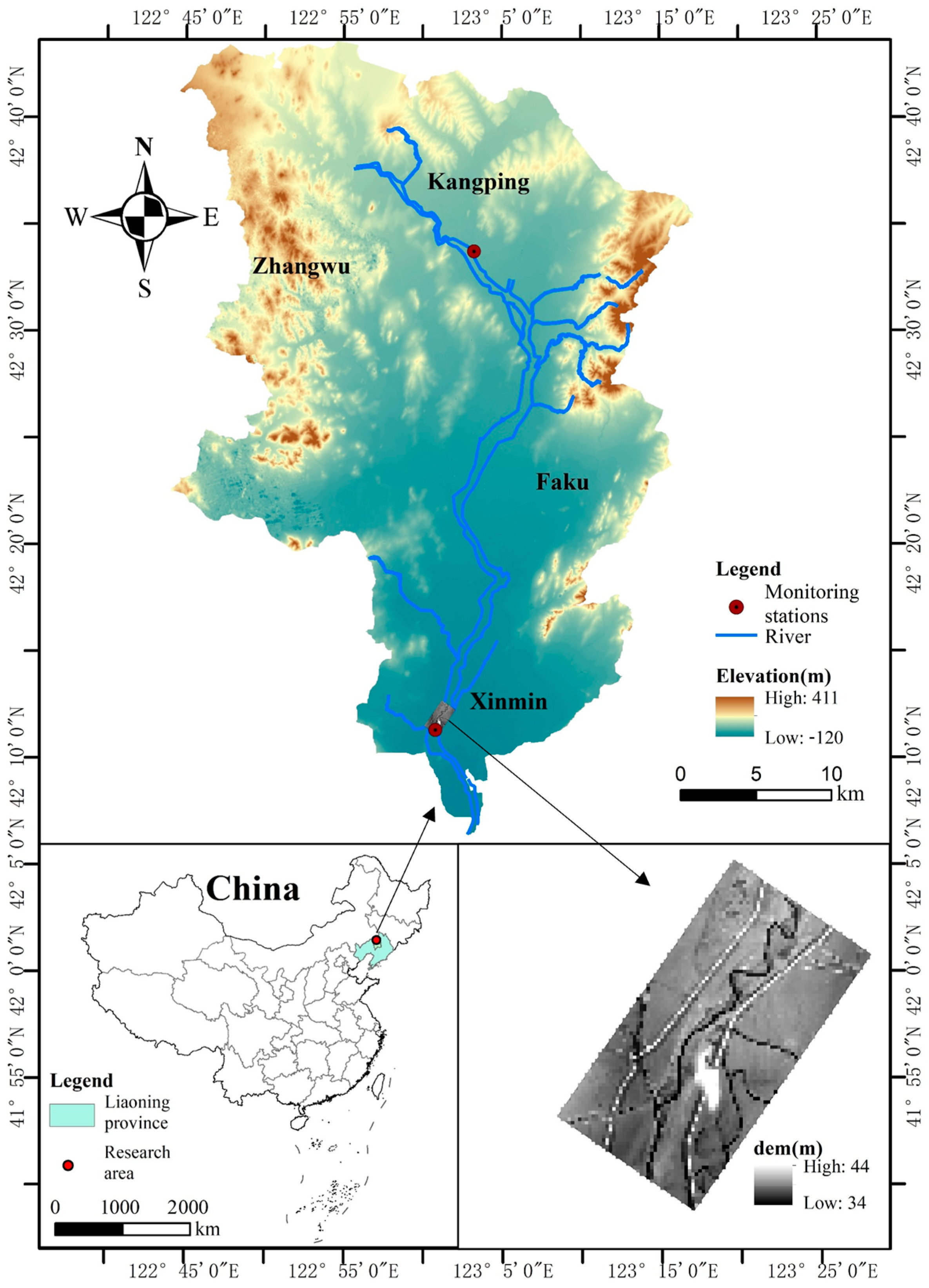
In this study, a section of the Xiushui River was selected as the study area (Figure 1). The Xiushui River, a primary tributary of the middle and lower reaches of the Liao River, originates in southwest Kangping County, Liaoning Province. It flows through Zhangwu County in Fuxin City and the counties of Faku and Xinmin in Shenyang City before joining the Liao River near Guanjia Wopu Village in Xinmin County. The Xiushui River Basin spans 135.65 km in length and covers approximately 1994.2 square kilometers in drainage area. The basin’s morphology is broader in the northwest and narrower in the southeast, with terrain sloping from northwest to southeast, relatively flat in the middle and lower reaches. The river is known for its winding and meandering course, with a riverbed mainly composed of sandy loam soil that offers weak resistance to erosion. During flood periods, the river undergoes significant sedimentation and erosion changes, with rapid fluctuations in water levels, making it susceptible to flooding influenced by the Liao River. This study focuses on the downstream section of the Xiushui River as a case study. Due to climatic influences, floods in the Liao River basin occur frequently, with major floods every (7 to 8) years and minor floods every (2 to 3) years. However, the scarcity of monitoring stations in the study area has led to limited hydrological data, presenting challenges and opportunities for water depth prediction and simulation under data scarcity conditions.

The essential data required for constructing the model in this study included digital elevation model (DEM) data, river data, 1-h rainfall flow depth data measured hourly from 6 July 2022 to 28 July 2022, along with land-use data (

Table 1. Summary of datasets used in this study.

Data Name	Source	Resolution	Coverage	Period
Precipitation	Rain gauge	1 h	1 site	24 h
DEM	Government	1 m	Global	—
Flow	Monitoring station	1 h	1 site	24 h
Water depth	Monitoring station	1 h	1 site	24 h

). The primary flow monitoring station used was Gongzhutun Station. The data were relatively complete, and all were formatted in the WGS-84 coordinate system, using the UTM zone 49 N projection for the planar coordinate system. Land-use data were instrumental in configuring the model parameters. The DEM and land-use data helped quantify the influence of underlying surfaces on river depth simulations, while flow and rainfall data were used for model calibration and validation.

To construct a two-dimensional hydrodynamic model for the downstream area of the study, it was necessary to obtain the flow conditions of a tributary under specified rainfall scenarios. Due to the scarcity of real-time tributary flow data, a constant flow rate of 5.37 m³/s was used as the input for the two-dimensional hydrodynamic model. This value was derived from a regional hydrological report covering the flood season (June to August) from 2020 to 2022 in Shenyang City, representing the average flow rate observed at a nearby monitoring station during flood conditions.

3. Methodology

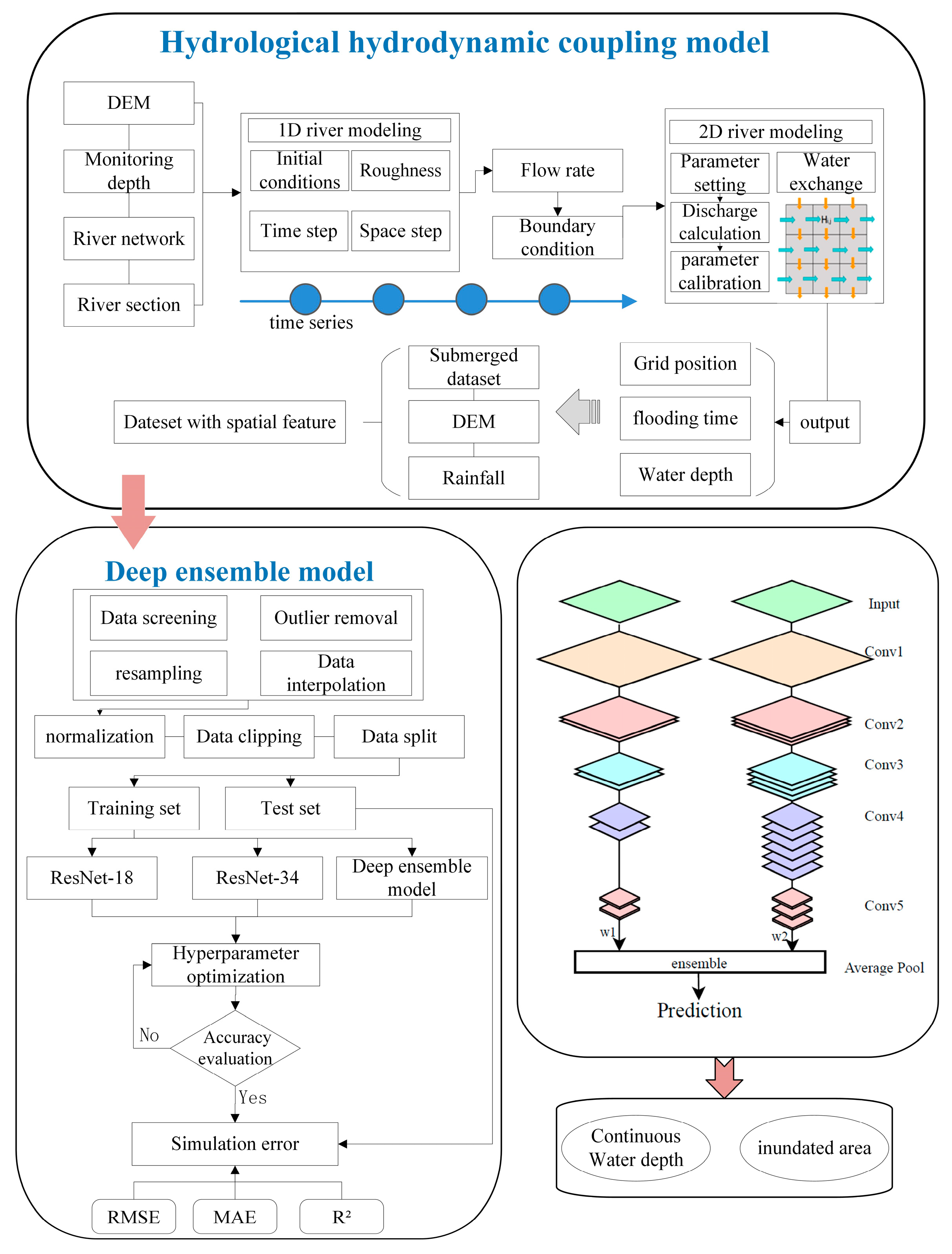
As shown in Figure 2, this study incorporated two primary types of models: a coupled hydrodynamic–hydrological model based on physical processes and a depth-integrated model driven by the simulation results of the former.

The main steps of the research process are outlined as follows:

Step 1: Construct a one-dimensional river model for the upstream area of the study region to obtain the time-series flow processes at the upstream and downstream boundary points.

Step 2: Use the time-series flow process obtained from Step 1 as boundary conditions to drive the two-dimensional hydrodynamic model (LISFLOOD) for downstream model construction, generating spatially distributed time-series flood depth inundation sequences.

Step 3: Utilize the spatially distributed time-series flood depth inundation sequences from Step 2, combined with factors influencing the flood propagation process, such as rainfall and the DEM to form a spatial feature dataset.

Step 4: Construct, train, and optimize the deep learning (DL) model.

Step 5: Use real-time monitoring data to drive the trained DL model for river water depth inundation calculations.

3.1. Constructing Spatial Feature Dataset

The spatial feature dataset included outputs from the hydrodynamic coupling model, rainfall sequences, and DEM. To accommodate the stochastic nature of rainfall event duration, rainfall uniformity was enhanced to ensure consistency in the feature dimensions of the constructed dataset. The data preparation involved cleaning and filtering the rainfall data to remove anomalies and matching the spatiotemporal dimensions of river water depth, terrain data, and rainfall amounts.

3.1.1. One-Dimensional Channel Model

The Storm Water Management Model (SWMM) is well-suited for simulating the hydraulic behavior of surface runoff, rivers, and drainage networks [21,22]. While other one-dimensional river models typically assume consistent cross-sectional shapes along a river reach, the SWMM offers the flexibility to assign different cross-sectional shapes to different segments. This characteristic can pose challenges for modeling natural rivers with highly variable geometry. However, in our study area, with an urban river section with relatively uniform and gently varying cross-sections, this flexibility becomes advantageous. Therefore, the SWMM was selected as a suitable tool for simulating the upstream one-dimensional river flows in this context. Using linear river data, breakpoints in the river channel are identified where nodes are segmented and extracted, and the flow direction of each segment is determined by the elevation of the nodes. The shape and width of the conduit are determined based on the river section at each turning point. Each segment of the conduit in the river model includes an inlet and an outlet. The one-dimensional river modeling begins at the measured points, starting with the inlet provided with measured flow rates and connecting to the outlet of the next conduit segment. The SWMM 5.1 software was used to simulate the upper section of the river, with parameters including cross-sectional characteristics, bottom elevation, and friction coefficient [23].

The numerical solution method employs the finite volume method to simulate changes in water level and flow velocity within the river channel over a time step. The Saint-Venant equations are used to model the flow process in the river channel, as outlined below. Model parameters are determined based on the inflow and outflow processes of the Sanjiazi Reservoir. By abstracting and simplifying river flow into a one-dimensional channel composed of nodal sections and conduits, the model calculates the final node outflow based on upstream inflow.

$${\displaystyle \frac{\partial \mathrm{A}}{\partial \mathrm{t}}}+{\displaystyle \frac{\partial \mathrm{Q}}{\partial \mathrm{x}}}=0$$

(1)

$${\displaystyle \frac{\partial \mathrm{Q}}{\partial \mathrm{t}}}+{\displaystyle \frac{\partial \left(\frac{{\mathrm{Q}}^2}{\mathrm{A}}\right)}{\partial \mathrm{x}}}+\mathrm{g}\mathrm{A}{\displaystyle \frac{\partial \mathrm{H}}{\partial \mathrm{x}}}+\mathrm{g}\mathrm{A}{\mathrm{S}}_{\mathrm{f}}=0$$

(2)

where A represents the cross-sectional area of the river section, Q represents the discharge of the river, H represents the height of the water, t represents time, Z represents the inner bottom elevation, Y represents the channel depth, ${\mathrm{S}}_{\mathrm{f}}$ represents friction slope, and g represents gravitational acceleration.

3.1.2. Two-Dimensional Channel Model

The LISFLOOD is a hydrodynamic model that effectively utilizes geographic, hydrological, and meteorological data [23]. It was employed to generate the training samples for the data-driven predictive models considered in this study. The model uses DEM grid units as the smallest computational units and incorporates the outflow rate from the one-dimensional river model in the upper section of the study area as primary input data, along with the rainfall and DEM. Land-use data were also used to set the initial parameters of the model. Within the research area, tributary inflow is present, and boundary conditions for this inflow were established. Historical water depth monitoring data from the Gongzhutun Station were used for parameter calibration to select a model suitable for this area. The model uses one-dimensional Saint-Venant equations to describe the water flow within the river channel. When water overflows the embankments, it flows from the river channel into the adjacent floodplains, establishing real-time bidirectional water exchange with these floodplains. The shallow water equation is used to calculate the diffusion of water flow on a two-dimensional surface, yielding spatially distributed time-series water depth results. This data-to-hydraulic modeling and simulation process is illustrated in Figure 3.

Continuity equation:

$$\mathrm{B}{\displaystyle \frac{\partial \mathrm{Z}}{\partial \mathrm{t}}}+{\displaystyle \frac{\partial \mathrm{Q}}{\partial \mathrm{x}}}=0$$

(3)

Shallow water equation:

$${\displaystyle \frac{\partial \mathrm{Q}}{\partial \mathrm{t}}}+\mathrm{u}{\displaystyle \frac{\partial \mathrm{Q}}{\partial \mathrm{x}}}+\mathrm{g}\mathrm{A}{\displaystyle \frac{\partial \mathrm{Z}}{\partial \mathrm{x}}}+\mathrm{g}{\displaystyle \frac{{\mathrm{n}}^2\mathrm{Q}\left|\mathrm{u}\right|}{{\mathrm{R}}^{\frac{4}{3}}}}=0$$

(4)

Here, Z represents water level, Q represents discharge, B represents the channel section width, $\mathrm{u}$ represents water velocity in the channel section, $\mathrm{A}$ represents the area of the channel section, $\mathrm{n}$ represents channel roughness, $\mathrm{g}$ represents gravitational acceleration, and $\mathrm{R}$ represents the hydraulic radius.

3.1.3. Constructing Physical Coupling Model

The flow of water in drainage systems is complex, involving multidimensional and multiscale exchanges. One-dimensional hydrodynamic models offer the advantages of simple computational structures and high computational efficiency. In contrast, two-dimensional hydrodynamic models provide spatiotemporal sequences of water depth in the study area but involve extensive physical computation, resulting in lower computational efficiency. Coupling one-dimensional and two-dimensional models exploits the advantages of both, making it a strategic choice for simulating flood processes in areas with extensive spatial coverage and complex spatial correlations.

The coupling methods used in this study include one-way coupling between the one-dimensional river model and the two-dimensional hydrodynamic model and coupling between the output results of the two-dimensional model and the ML model.

Multiple coupling methods are used for simulating urban river flow using hydrodynamic models, categorized based on directional connection mechanisms into lateral and longitudinal coupling, and based on flow exchange characteristics into one-way and two-way coupling. In this study, unidirectional coupling was used in the modeling according to the physical characteristics of the water flow. Firstly, the one-dimensional channel model constructed with the SWMM was established, as well as the longitudinal unidirectional coupling of the two-dimensional channel in the main study area, where the initial velocity component in the y-direction of the water flow is neglected and the water volume is allocated according to the two-dimensional surface elevation after the coupling is established. Utilizing the terrain characteristics, unidirectional water exchange between the river channel and floodplains was constructed, and water depth calculations were performed using the water quantity calculation solver in LISFLOOD, resulting in spatially distributed time-series water depth data for the floodplains. This method allows for the detailed simulation of flood-prone areas.

The coupling of hydrodynamic and ML models does not directly use the output results of the physical model as the boundary conditions for the ML model. Instead, it involves coupling the spatial water depth results output by the model on a per-grid basis, thereby achieving vertical data transfer at each grid point. After selecting and combining data, a spatial feature dataset was formed to train the ML model.

3.2. Data Preprocessing

First, rainfall and water depth data were synchronized to ensure consistent temporal resolution before integration with DEM data to create a spatial dataset for the study area. A threshold of 0.1 m was applied to filter water depth values; depths below this threshold increased the model output to zero. This adjustment was made because areas with such shallow flood depths typically have brief flood durations and undergo rapid changes in flood state, complicating the generation of sufficient training samples for ML models to accurately describe highly variable flood processes. Second, the output water depth data from the hydrodynamic model were checked for missing values and outliers. Data from regions showing outliers were removed, and interpolation was used for resampling to ensure comprehensive coverage and uniformity. Given the varying units and ranges of features in the datasets, direct use of raw data could impact the reliability of the model. Therefore, normalization was employed to eliminate the dimensional influence of these features, using the min-max scaling method to scale data between zero and one. This process created a comprehensive water depth database for the study area.

The outputs of the hydrodynamic model were then evaluated, and rainfall and DEM data were combined to form a dual-channel input. To facilitate analysis, slices sized 224 × 224 were cropped, generating a spatial dataset comprising 8050 samples. This cropping approach was adopted for several reasons: First, it standardizes the input size of the water depth data as 224 × 224, which is a common input dimension for deep learning models, ensuring compatibility with standard architectures. Second, cropping reduces image resolution, which lowers memory usage and computational cost, thereby accelerating the training process. Additionally, cropping eliminates irrelevant background areas, such as land, allowing the model to focus on water regions and reducing noise interference, which enhances the model’s performance and accuracy.

3.3. Construct Spatial Prediction Model Using Deep Learning

An ensemble model combines predictions from various models to make a final prediction. A deep ensemble model integrates the advantages of DL models and ensemble learning, leveraging multiple models for a combined computation [20]. A residual network (ResNet) is a type of deep convolutional neural network designed to address the vanishing gradient and exploding gradient problems in deep neural networks. The convolution operation is shown in Figure 4c. Both ResNet18 and ResNet34, based on residual networks, incorporate residual blocks with skip connections that bypass nonlinear transformations between layers, effectively mitigating the vanishing gradient problem in deep neural networks. The residual block is presented in Figure 4b. ResNet18, with 18 layers and fewer parameters, offers a lightweight architecture suitable for data-scarce scenarios, while ResNet34, with 34 layers, provides stronger feature extraction for complex flood dynamics, though it requires greater computational resources [20]. These architectures enhance the deep ensemble model’s ability to predict spatially distributed water depths by leveraging their complementary strengths.

$${\mathrm{Y}}_{\mathrm{i}}=\mathrm{F}\left({\mathrm{x}}_{\mathrm{i}},{\mathrm{W}}_{\mathrm{i}}\right)+\mathrm{h}\left({\mathrm{x}}_{\mathrm{i}}\right)$$

(5)

$${\mathrm{x}}_{\mathrm{i}+1}=\mathrm{f}\left({\mathrm{y}}_{\mathrm{i}}\right)$$

(6)

where ${\mathrm{x}}_{\mathrm{i}}$ and ${\mathrm{x}}_{\mathrm{i}+1}$ represent the input and output of the i-th residual unit, F represents the residual function, ${\mathrm{W}}_{\mathrm{i}}$ represents the parameters of the convolution layer, $\mathrm{h}({\mathrm{x}}_{\mathrm{i}}) = {\mathrm{x}}_{\mathrm{i}}$ denotes the addition operation, and $\mathrm{f}$ represents the ReLu activation function.

The integrated model designed for water depth modeling is depicted in the following figure. This architecture significantly differs from the physical model, mainly because the computation mechanisms for water depth are different and mapping water depth is not a straightforward image analysis task. Our method combines multiple DL models to enhance overall accuracy and robustness. The input layer of the ResNet model receives rainfall and DEM data for the study area. The model consists of a series of convolutional layers, batch normalization layers, activation functions, downsampling operations, and residual blocks. The forward method defines the forward propagation logic of the entire model. The output layer includes nodes equal to the number of units in the simulation domain. Subsequently, a weighted approach integrates the two constructed ResNet models to obtain the river plane water depth prediction model used in this study. The main body of the deep ensemble model is shown in Figure 4. The model uses an end-to-end approach, where the Encoder transforms the relationship between the rainfall, DEM, and water depth into a mathematical problem, and the Decoder is responsible for solving this problem and providing the water depth prediction for the study area.

3.4. Model Training and Evaluation

To measure the accuracy of the output results from the physical model, we optimized the model results based on real-time water depth monitoring data using the Nash–Sutcliffe efficiency coefficient as an evaluation metric.

$$\mathrm{NSE}=1-{\displaystyle \frac{\sum _{\mathrm{t}=1}^{\mathrm{T}} {\left({\mathrm{D}}_{\mathrm{obs}}^{\mathrm{t}}-{\mathrm{D}}_{\mathrm{sim}}^{\mathrm{t}}\right)}^2}{\sum _{\mathrm{t}=1}^{\mathrm{T}} {\left({\mathrm{D}}_{\mathrm{obs}}^{\mathrm{t}}-\overline{{\mathrm{D}}_{\mathrm{obs}}}\right)}^2}}$$

(7)

where ${\mathrm{D}}_{\mathrm{obs}}^{\mathrm{t}}$ is a one- and two-dimensional coupled river model output, ${\mathrm{D}}_{\mathrm{sim}}^{\mathrm{t}}$ is a deep ensemble model predicting water depth, and $\overline{{\mathrm{D}}_{\mathrm{obs}}}$ is the mean value of the water depth from a one- and two-dimensional channel model.

To evaluate the capability of the proposed deep ensemble model to simulate the distribution of two-dimensional water depth, we directly compared the predicted water depth results from the DL model with the output results from the LISFLOOD physical model. Additionally, to validate the performance of the deep ensemble model, it was compared with predictions from the individual integrated models. For hyperparameter tuning, the Adam optimization algorithm was employed, utilizing the concept of adaptive learning rates. This approach allows each parameter to be updated with different scales during the training process, enhancing the efficiency and accuracy of model adjustments. The model with the optimal parameters was then applied to the testing dataset. To quantify the performance improvements over multiple iterations, evaluation metrics, including the root mean square error (RMSE), mean absolute error (MAE), and the coefficient of determination (R²), were employed. Model performance was gradually improved through multiple iterations. The equations for these evaluation metrics are as follows:

$$\mathrm{RMSE}=\sqrt{{\displaystyle \frac{{\sum }_{\mathrm{i}=1}^{\mathrm{n}}({\mathrm{X}}_{\mathrm{o},\mathrm{i}}-{\mathrm{X}}_{\mathrm{m},\mathrm{i}}{)}^2}{\mathrm{n}}}}$$

(8)

$$\mathrm{MAE}={\displaystyle \frac{1}{\mathrm{n}}}\sum _{\mathrm{i}=1}^{\mathrm{n}}\left|{\mathrm{X}}_{\mathrm{o},\mathrm{i}}-{\mathrm{X}}_{\mathrm{m},\mathrm{i}}\right|$$

(9)

$${\mathrm{R}}^2={\displaystyle \frac{\sum _{\mathrm{i}=1}^{\mathrm{n}} (\stackrel{\wedge }{{\mathrm{X}}_{\mathrm{m},\mathrm{i}}}-\overline{{\mathrm{X}}_{\mathrm{o},\mathrm{i}}}{)}^2}{\sum _{\mathrm{i}=1}^{\mathrm{n}} ({\mathrm{X}}_{\mathrm{o},\mathrm{i}}-\overline{{\mathrm{X}}_{\mathrm{o},\mathrm{i}}}{)}^2}}$$

(10)

$$\mathrm{E}=1-{\displaystyle \frac{{\sum }_{\mathrm{i}=1}^{\mathrm{n}}({\mathrm{X}}_{\mathrm{o},\mathrm{i}}-\stackrel{\wedge }{{\mathrm{X}}_{\mathrm{m},\mathrm{i}}}{)}^2}{{\sum }_{\mathrm{i}=1}^{\mathrm{n}}({\mathrm{X}}_{\mathrm{o},\mathrm{i}}-\overline{{\mathrm{X}}_{\mathrm{o},\mathrm{i}}}{)}^2}}$$

(11)

where ${\mathrm{X}}_{\mathrm{o},\mathrm{i}}$ represents observed water depth, $\stackrel{\wedge }{{\mathrm{X}}_{\mathrm{m},\mathrm{i}}}$ represents simulated water depth, and $\overline{{\mathrm{X}}_{\mathrm{o},\mathrm{i}}}$ represents observed mean water depth.

4. Results and Discussion

The two-dimensional hydrodynamic model conducted 98 simulations based on two rainfall scenarios. The constructed spatial feature dataset was divided, with 70% used as the training set and 30% as the unseen dataset, to evaluate the trained and validated model performance. This study assessed the performance of the depth-integrated model, ResNet18, and ResNet34 ML algorithms using metrics such as MAE, RMSE, and R². To ensure the fairness and efficiency of the experiment, we completed all experiments on the same computer equipped with an Intel Core i5-12400 (2.5 GHz) CPU and 16 GB of memory. The DL-based works were implemented using the PyTorch framework and executed on a single NVIDIA GeForce RTX 3090 GPU (24 GB memory). The model utilized the Adam optimization algorithm with a learning rate set to 0.001. The loss function employed was mean squared error, and the batch size was set to 4.

4.1. Physical Model Simulation Results

4.1.1. Time-Varying Discharge of One-Dimensional Channel Model

To simulate downstream flood scenarios in the study area and demonstrate the efficacy of the depth-integrated model, it was necessary to generate sufficient input flow and output water depth data as the driving sources. The SWMM was used to construct a one-dimensional river model in the upper reaches of the study area, and the model parameters were calibrated using hourly measurement data from the Qijiazi Reservoir. The Nash–Sutcliffe efficiency coefficients for the rainfall events on 6 July 2022 (here-after referred to as the 6 July Flooding Event) and 28 July 2022 (hereafter referred to as the 28 July Flooding Event) were 0.89 and 0.83, respectively.

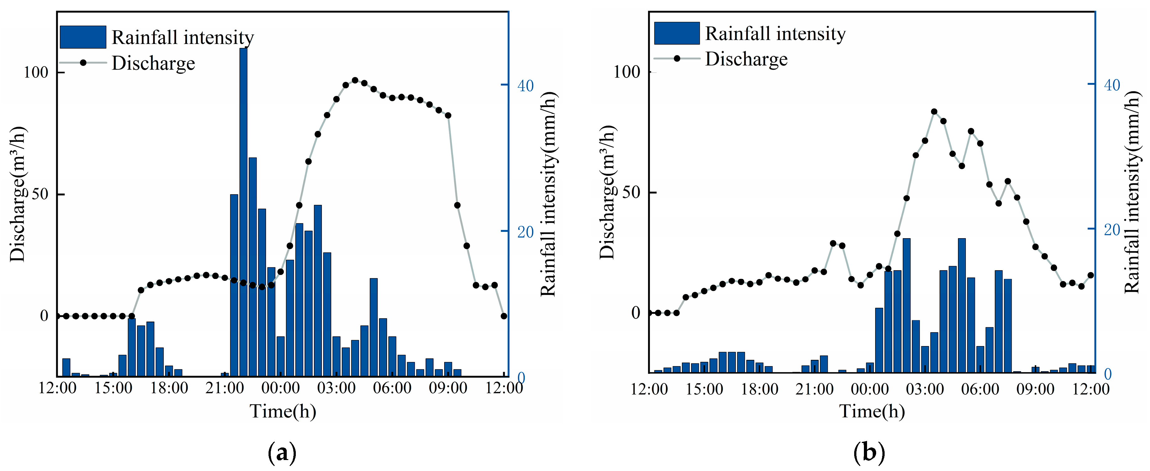
Additionally, 24 h rainfall data measured hourly for 6 July and 28 July 2022 served as the temporal flow input for the lower section of the main study area. As shown in Figure 5, the total rainfall intensity of the 6 July event exceeded that of the 28 July event. On 6 July, the rainfall intensity in the study area sharply increased from 18:00 to 21:00, leading to a rapid increase in river flow. The main reason for this increase in river flow was external inflow, causing a delayed response to the rainfall. From midnight to 4:00 a.m. on 7 July, the river flow sharply increased, peaking at approximately 96 m³/h at 4:00 a.m. As the rainfall intensity gradually decreased, the river flow decreased and stabilized at approximately 85 m³/h. Rainfall stopped at approximately 23:00 on 6 July, and river flow began to decline at approximately 9:00 on 8 July, eventually returning to zero.

Compared to the rainfall on 6 July 2022, the rainfall on 28 July 2022 was overall lower. It displayed three nearly identical peaks, with the maximum rainfall intensity reaching 18.6 mm/h. The river flow peaked at 3 a.m. on 29 July, reaching a maximum flow rate of 83 m³/h. Subsequently, the river flow exhibited a lagging fluctuation pattern as the rainfall continued. After 9 a.m. on 29 July, as the rainfall intensity decreased, the river flow eventually stabilized at a discharge rate of approximately 10 m³/h after several hours.

4.1.2. Spatial Distribution Depth of Two-Dimensional Channel Model

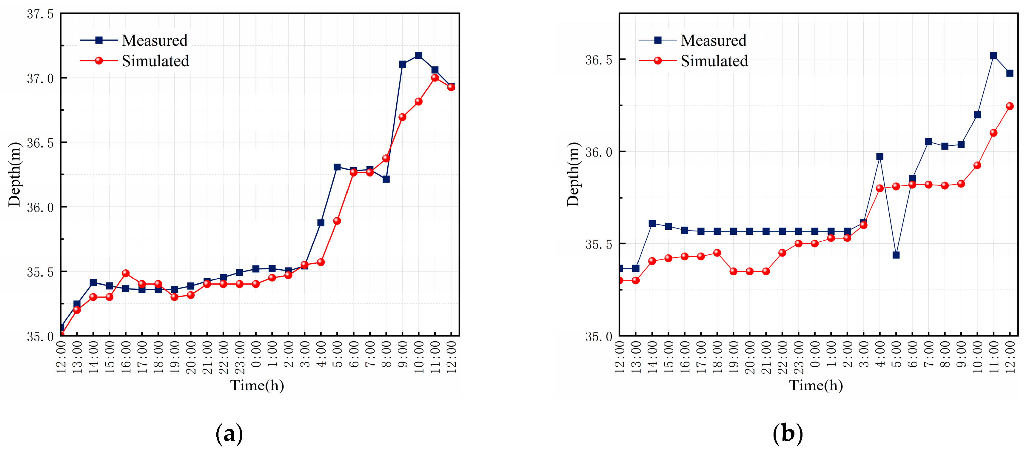
To ensure the accuracy of the dataset used in the deep ensemble model, we optimized the results of the two-dimensional river model in the downstream study area. Given the small size of the downstream study area and the presence of a tributary, a constant flow rate of 5.37 m³/s was used as the input. We selected the Gongzhutun Station as a typical hydrological station to verify the accuracy of the two-dimensional river model. The measured water depth at Gongzhutun Station during the 6 July 2022 rainfall event was used for model parameter optimization. The main adjusted parameters are presented in

Table 2. Parametric values of the hydrodynamic model.

Parameter	Value
Manning coefficient of impermeable area	0.03
Manning coefficient of permeable area	0.04
Infiltration attenuation constant (channel)	0.00001
Infiltration attenuation constant (channel sides)	0.00006

. These saved parameters were then used to simulate the 28 July 2022 rainfall event. A comparison of the output water depth time-series of the model with the actual measured water depth time-series for both rainfall events is shown in Figure 6. Error was quantified using RMSE, with an RMSE of 0.112 for the July 6th rainfall event and an RMSE of 0.27 for the July 28th rainfall event.

4.2. Spatial Prediction Model Simulation Results

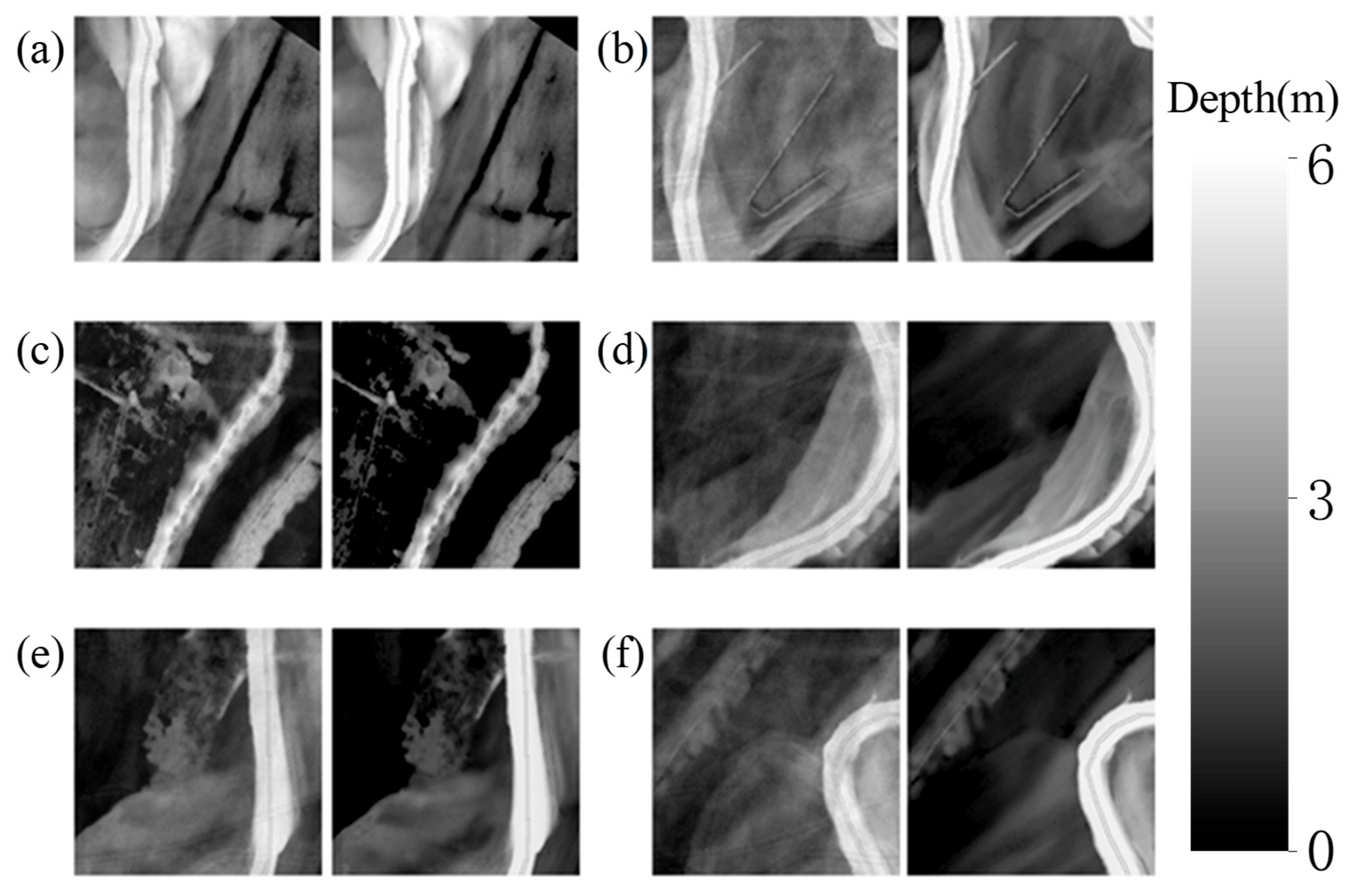
To demonstrate the efficacy of the deep ensemble method, we replicated the impact of the rainfall event on 6 July 2022,on river water depth and compared these results with those obtained using the LISFLOOD method.

Figure 7 presents the sliced and refined simulation results of the 6 July 2022 rainfall event, which lasted approximately 12 h. When focusing on the zoomed-in areas, the deep ensemble model accurately captured the inundation extent and depth of the river, showing an almost identical visual representation to that of the physical model. The model also accurately simulated riverbank flooding, closely matching with the inundation maps predicted by the physical model during the flood stage. This demonstrates that the deep ensemble model used in this study can accurately simulate both the temporal and spatial variations in water depth within the study area. Randomly selected water depth maps, derived from different scenarios trained on the water depth database, showed minimal differences in the overall water depth output results, affirming the capability of the deep ensemble model to effectively predict inundation scenarios.

To systematically evaluate the error, we computed the deviation between the predicted and actual water depths for each pixel unit. This deviation was calculated as the difference between the predicted and actual water depth matrices. Figure 8 illustrates the deviation in the spatial distribution of water depth. The results indicate that the water depth predicted by the DL model closely aligns with the actual situation, with a low probability of predicting outliers. Calculations indicate that over 98% of the total number of cells show a water depth difference within 0.15 m. Overall, these results further confirm that the ensemble model can effectively reproduce the spatial distribution of water depth, underscoring its utility in flood modeling and risk management.

Figure 9 illustrates the accuracies of the three ML models in the simulation. The goodness of fit, measured by R², was 0.95 for the deep ensemble model, 0.76 for ResNet34, and 0.60 for ResNet18. The RMSE values were 0.04, 0.07, and 0.09, respectively. The red line in each subplot of Figure 9 represents the fitting line, indicating the ideal 1:1 relationship between predicted and estimated water depths, which helps assess the models’ performance. The results indicate that all three models provided satisfactory water depth simulation results for the river channel in the study area. The deep ensemble model outperformed the others, followed by ResNet34 and ResNet18. Compared to ResNet34 and ResNet18, the deep ensemble model shows a 25% and 58% improvement in the goodness of fit R² and a reduction of 42% and 55% in RMSE, respectively.

This study also calculated the predictive performance of the deep ensemble, ResNet18, and ResNet34 models for the 6 July 2022 rainfall event. The average values of the pixel-wise water depth error metrics, including MAE, RMSE, and R², were compiled, as listed in

Table 3. Comparison of water depth performances from different models.

Model	Deep Ensemble Model	ResNet18	ResNet34
MAE	0.02 m	0.05 m	0.03 m
RMSE	0.04 m	0.09 m	0.07 m
R2	0.95	0.6	0.76

. In cases where the model water depth difference is less than 0.15 m, such instances account for over 97% of the total units. The deep ensemble model exhibited superior performance in simulating water depth, with over 99.8% of the area having a water depth difference of less than 0.15 m.

4.3. Simulated Performance

The evaluation of model performance consists of two stages: testing and validation. In the testing stage, the metrics used were the R² index, RMSE, and MAE. During the validation stage, specific time-series data were selected to evaluate the performance of the model. First, to assess the ability of the model to predict changes in inundation depth, the difference between the predicted and the physically modeled water levels was calculated. Second, the duration of use of the DL model for water depth prediction was monitored and compared with that of the physical model.

A comparison of the simulation speeds for the entire flood process, based on the same number of grids and a 12 h rainfall scenario on the same computing device, is detailed in

Table 4. Calculation speed comparison from different models.

Model	Simulation Calculation Time
LISFLOOD	181.4 min
Deep ensemble model	3.24 min

. Employing the deep ensemble model for river water depth prediction significantly improved the simulation speed, highlighting its efficiency and effectiveness in flood modeling.

5. Conclusions

This study proposed a novel approach for accurately and rapidly predicting river water depth in areas with limited monitoring and sparse data. The following conclusions can be drawn from this study:

(1) ResNet18, ResNet34, and a deep ensemble model were used for flood water depth prediction. The results indicate that the deep ensemble model outperformed both ResNet18 and ResNet34 in terms of prediction accuracy and model performance, achieving a prediction accuracy of 99.84%. The number of cells with significant errors was relatively small and difficult to discern on the map. Future research could involve identifying critical locations wherein cells with large errors occur and using single-point water depth prediction models for precise depth estimation.

(2) In areas with limited river monitoring stations, river depth can be predicted using multiple coupling methods. Starting from one monitoring station, a rapid one-dimensional river simulation model was constructed based on river characteristics to obtain the outflow discharge, which served as the boundary condition for the main downstream research area. Subsequently, a two-dimensional river model for the main research area was constructed to obtain the spatial distribution sequence of water depth, thereby achieving a segmented simulation of the continuous river channel.

(3) In the event of sudden heavy rainfall, only the input rainfall data must be updated in the proposed multi-coupling model to rapidly generate a spatial inundation situation in the main research area. Compared with traditional hydrodynamic models, the computational speed of the proposed model is significantly higher; this aids in early planning to alleviate flooding and implement disaster relief measures.

This study effectively employs a coupled model integrating one-dimensional and two-dimensional hydrodynamic models with machine learning techniques to achieve the robust prediction of urban river water depths across large-scale regions, adeptly adapting to varying rainfall conditions and surface characteristics. The model’s inputs include spatially and temporally distributed flood depth sequences generated by the two-dimensional hydrodynamic model, alongside rainfall sequences and digital elevation model data. The output consists of predicted water depth distributions, with a root mean square error (RMSE) of 0.04 and a coefficient of determination (R²) of 0.95, demonstrating exceptionally high predictive accuracy. However, the current approach does not fully account for water flow exchanges at segmented grid boundaries, which may affect the continuity of water depth predictions across interconnected regions. Additionally, due to the lack of field-measured data, this study utilized time-series flow outputs from the SWMM as boundary conditions to drive the two-dimensional hydrodynamic model, generating the water depth dataset. Future research should prioritize addressing boundary flow interactions, integrating multi-source field data, and considering additional factors influencing river water depth, such as surface roughness and the efficiency of urban drainage systems. By conducting simulations under diverse multi-factor scenarios, the model’s interpretability and predictive performance can be enhanced, enabling its broader application in various urban flood management contexts.

References

- Mukherji, A. Climate Change 2023 Synthesis Report; 2023. Available online: https://cgspace.cgiar.org/items/7e70f98b-3a47-4881-8d8a-0e988c594ef4 (accessed on 17 July 2025).
- Luo, P.; Luo, M.; Li, F.; Qi, X.; Huo, A.; Wang, Z.; He, B.; Takara, K.; Nover, D.; Wang, Y. Urban Flood Numerical Simulation: Research, Methods and Future Perspectives. Environ. Model. Softw. 2022, 156, 105478. [Google Scholar] [CrossRef]
- Ye, C.; Xu, Z.; Lei, X.; Zhang, R.; Chu, Q.; Li, P.; Ban, C. Assessment of the Impact of Urban Water System Scheduling on Urban Flooding by Using Coupled Hydrological and Hydrodynamic Model in Fuzhou City, China. J. Environ. Manag. 2022, 321, 115935. [Google Scholar] [CrossRef] [PubMed]
- Cao, Y.; Ye, Y.; Liang, L.; Zhao, H.; Jiang, Y.; Wang, H.; Yi, Z.; Shang, Y.; Yan, D. A Modified Particle Filter-Based Data Assimilation Method for a High-Precision 2-D Hydrodynamic Model Considering Spatial-Temporal Variability of Roughness: Simulation of Dam-Break Flood Inundation. J. Water Resour. Res. 2019, 55, 6049–6068. [Google Scholar] [CrossRef]
- Ye, C.; Xu, Z.; Lei, X.; Zhang, R.; Chu, Q. Inundation Simulation for Urban Drainage Basin With Storm Sewer System. J. Hydrol. 2000, 234, 21–37. [Google Scholar] [CrossRef]
- Neal, J.; Schumann, G.; Bates, P. A Subgrid Channel Model for Simulating River Hydraulics and Floodplain Inundation over Large and Data Sparse Areas. Water Resour. Res. 2012, 48. [Google Scholar] [CrossRef]
- Felder, G.; Zischg, A.; Weingartner, R. The Effect of Coupling Hydrologic and Hydrodynamic Models on Probable Maximum Flood Estimation. J. Hydrol. 2017, 550, 157–165. [Google Scholar] [CrossRef]
- Hdeib, R.; Abdallah, C.; Colin, F.; Brocca, L.; Moussa, R. Constraining Coupled Hydrological-Hydraulic Flood Model by Past Storm Events and Post-Event Measurements in Data-Sparse Regions. J. Hydrol. 2018, 565, 160–176. [Google Scholar] [CrossRef]
- Li, W.; Lin, K.; Zhao, T.; Lan, T.; Chen, X.; Du, H.; Chen, H. Risk Assessment and Sensitivity Analysis of Flash Floods in Ungauged Basins Using Coupled Hydrologic and Hydrodynamic Models. J. Hydrol. 2019, 572, 108–120. [Google Scholar] [CrossRef]
- Kabir, S.; Patidar, S.; Xia, X.; Liang, Q.; Neal, J.; Pender, G. A Deep Convolutional Neural Network Model for Rapid Prediction of Fluvial Flood Inundation. J. Hydrol. 2020, 590, 125481. [Google Scholar] [CrossRef]
- Costa, D.; Burlando, P.; Liong, S.Y. Coupling spatially distributed river and groundwater transport models to investigate contaminant dynamics at river corridor scales. Environ. Model. Softw. 2016, 86, 91–110. [Google Scholar] [CrossRef]
- Shaw, J.; Kesserwani, G.; Neal, J.; Bates, P.; Sharifian, M.K. LISFLOOD-FP 8.0: The New Discontinuous Galerkin Shallow-Water Solver For Multi-Core CPUs and GPUs. Geosci. Model Dev. 2021, 14, 3577–3602. [Google Scholar] [CrossRef]
- Bermúdez, M.; Cea, L.; Puertas, J. A Rapid Flood Inundation Model For Hazard Mapping Based on Least Squares Support Vector Machine Regression. J. Flood Risk Manag. 2019, 12, e12522. [Google Scholar] [CrossRef]
- Skoulikaris, C.; Nagkoulis, N. A Genetic Algorithm’s Novel Rainfall Distribution Method for Optimized Hydrological Modeling At Basin Scales. Engineering 2024, 26, 1295–1312. [Google Scholar] [CrossRef]
- Man, Y.; Yang, Q.; Shao, J.; Wang, G.; Bai, L.; Xue, Y. Enhanced LSTM Model for Daily Runoff Prediction in the Upper Huai River Basin, China. J. Eng. 2023, 24, 229–238. [Google Scholar] [CrossRef]
- Wan, X.; Yang, Q.; Jiang, P.; Zhong, P. A Hybrid Model for Real-Time Probabilistic Flood Forecasting Using Elman Neural Network with Heterogeneity of Error Distributions. Water Resour. Manag. 2019, 33, 4027–4050. [Google Scholar] [CrossRef]
- Huang, P.-C.; Hsu, K.-L.; Lee, K.T. Improvement of Two-Dimensional Flow-Depth Prediction Based on Neural Network Models By Preprocessing Hydrological and Geomorphological Data. Water Resour. Manag. 2021, 35, 1079–1100. [Google Scholar] [CrossRef]
- He, K.; Zhang, X.; Ren, S.; Sun, J. Deep residual learning for image recognition. In Proceedings of the IEEE Conference on Computer Vision and Pattern Recognition, Las Vegas, NV, USA, 27–30 June 2016; pp. 770–778. [Google Scholar]
- Ganaie, M.A.; Hu, M.; Malik, A.K.; Tanveer, M.; Suganthan, P.N. Ensemble Deep Learning: A Review. Eng. Appl. Artif. Intell. 2022, 115, 105151. [Google Scholar] [CrossRef]
- Ma, B.; Wu, Z.; Hu, C.; Wang, H.; Xu, H.; Yan, D.; Soomro, S. Process-Oriented SWMM Real-Time Correction and Urban Flood Dynamic Simulation. J. Hydrol. 2022, 605, 127269. [Google Scholar] [CrossRef]
- Feyen, L.; Vrugt, J.A.; Nualláin, B.Ó.; van der Knijff, J.; De Roo, A. Parameter Optimisation and Uncertainty Assessment for Large-Scale Streamflow Simulation with the LISFLOOD Model. J. Hydrol. 2007, 332, 276–289. [Google Scholar] [CrossRef]
- Rossman, L.A.; Huber, W.C. Storm Water Management Model Reference Manual Volume I–Hydrology; US Environmental Protection Agency: Washington, DC, USA, 2016; Volume 3.
- Van Der Knijff, J.; Younis, J.; De Roo, A.P.J. LISFLOOD: A GIS-Based Distributed Model for River Basin Scale Water Balance And Flood Simulation. Int. J. Geogr. Inf. Sci. 2010, 24, 189–212. [Google Scholar] [CrossRef]