Early Leak and Burst Detection in Water Pipeline Networks Using Machine Learning Approaches

Abstract

Leakages in water distribution networks pose a formidable challenge, often leading to substantial water wastage and escalating operational costs. Traditional methods for leak detection often fall short, particularly when dealing with complex or subtle data patterns. To address this, a comprehensive comparison of fourteen machine learning algorithms was conducted, with evaluation based on key performance metrics such as multi-class classification metrics, micro and macro averages, accuracy, precision, recall, and F1-score. The data, collected from an experimental site under leak, major leak, and no-leak scenarios, was used to perform multi-class classification. The results highlight the superiority of models such as Random Forest, K-Nearest Neighbours, and Decision Tree in detecting leaks with high accuracy and robustness. Multiple models effectively captured the nuances in the data and accurately predicted the presence of a leak, burst, or no leak, thus automating leak detection and contributing to water conservation efforts. This research demonstrates the practical benefits of applying machine learning models in water distribution systems, offering scalable solutions for real-time leak detection. Furthermore, it emphasises the role of machine learning in modernising infrastructure management, reducing water losses, and promoting the sustainability of water resources, while laying the groundwork for future advancements in predictive maintenance and resilience of water infrastructure.

1. Introduction

Historically, leak management in water distribution systems has relied on conventional methods such as acoustic detection (e.g., ground microphones, leak noise correlators, noise loggers), ground-penetrating radar, and thermal infrared imaging. These techniques, while valuable, are often labour-intensive, limited by environmental noise, and less effective in complex or buried infrastructures. Additionally, pressure management using Pressure Reducing Valves (PRVs) has traditionally been used to control leaks by minimizing excess system pressure. However, while effective, PRVs dissipate energy that could otherwise be recovered. Recent innovations such as Pumps-as-Turbines (PATs) offer a dual advantage by reducing pressure and recovering energy, enhancing both efficiency and sustainability. The industry has also explored preventative pipe replacement strategies, but these are often not economically justifiable compared to detection and repair or pressure reduction methods [1].

Despite the effectiveness of these methods in isolation, their limitations—such as cost inefficiency, difficulty in pinpointing exact leak locations, and their reactive nature—highlight the need for integrated, proactive solutions. Software-based (machine learning) and hardware-based approaches now play a critical role in optimizing leak management by combining hydraulic modelling, sensor data, and economic analysis. This integration allows for real-time monitoring, predictive maintenance, and economically optimal decision-making across leak detection, repair scheduling, and pressure management. By integrating conventional hydraulic models with machine learning and optimization frameworks, it is now possible to simultaneously evaluate the impact of pressure reduction and leak detection frequency. This holistic approach results in greater accuracy, better resource allocation, and reduced non-revenue water losses—benefits clearly demonstrated in recent case studies such as that by Hammond et al. (2024) [1], which found leak avoidance equivalent to 13–23% of customer demand and energy recovery equal to 10–11% of the system’s energy needs [1]. An Intelligent Water Network (IWN) is used to identify and react to potential events or behaviours in water networks prior to their prevalence, to mitigate or prevent their potential consequences [2]. This helps water authorities better understand what is happening in their water systems [3]. The benefits of IWN include helping to identify and repair leakages quickly, thereby saving water; improving customer service through early problem detection; aiding water authorities in better managing their pipe assets and equipment; and saving money by reducing water waste and avoiding major issues [3].

Joseph et al. [4] proposed a framework for the development of an IWN with the integration layers including sensing layer, communication layer, water system and operation layer, and application and prediction layer. The framework for an IWN is important because it enables more sustainable, efficient, and resilient urban water systems by integrating advanced technologies for improved management, resource optimisation, and informed decision making. Joseph et al. [5] provides a comprehensive overview of software- and hardware-based technologies for leak and burst detection in water pipeline networks. In particular, Joseph et al. [5] analysed and synthesised findings from the literature, including numerous studies to compare different leak detection methods based on factors like detection principle, sensitivity, accuracy, reliability, and ease of use. The efficacy of techniques for detecting anomalies, particularly related to pipe failures, leaks, and bursts, focusing on a case study in the Sunbury region of Victoria, Australia, was investigated by Joseph et al. (2024) [6]. This study utilised SCADA sensor technology to extract hydraulic characteristics and developed algorithms for leak and burst detection. Both logic-based and machine learning approaches were employed. Logic-based algorithms excelled at capturing straightforward anomalies, while machine learning techniques enhanced detection by learning from historical data and adapting to changing conditions.

Farajzadeh et al. [7] used machine learning to predict when pipes in municipal water distribution networks require repair. The methodology involves using a dataset of 1467 records of burst pipes from Saveh, Iran. Three one-class classification algorithms—OC-SVM, Isolation Forest, and Elliptic Envelope were trained on features like pipe size, type, location, etc. The models were assessed using standard performance metrics, namely accuracy, area under the receiver operating characteristic curve (AUC), and the F1-score. The AUC provides a comprehensive measure of the classifier’s ability to discriminate between classes across all decision thresholds, with values closer to 1 indicating superior separability. The F1-score, defined as the harmonic mean of precision and recall, offers a balanced evaluation of a model’s performance, particularly in scenarios involving imbalanced class distributions. Furthermore, Predict and Score Sample metrics were applied to both the original and balanced datasets to examine the models’ consistency and robustness across varying data conditions. This approach could assist municipalities in proactively maintaining water infrastructure and reducing water waste. McMillan et al. [8] present a hybrid machine learning framework for detecting and predicting leakage in water distribution systems at the district metered area (DMA) level. It uses one year of 15-minute interval flow data for over 2500 DMAs from Yorkshire Water, North Yorkshire, UK. The framework combines long short-term memory (LSTM) and recurrent neural networks (RNNs) for mean flow forecasting with Kalman filters (KFs) for residual forecasting. For leakage detection, the Isolation Forest algorithm is employed to identify outliers in the flow data, which correlates with known repairs.

Fagiani et al. [9] propose a framework for detecting leaks in water and natural gas grids using statistical modelling approaches. The authors used Gaussian Mixture Models (GMM), Hidden Markov Models (HMM), and One-Class Support Vector Machines (OC-SVM) to characterise normal consumption patterns and identify anomalies. A set of features is extracted from consumption data, including temporal features, and a modified sequential feature selection algorithm is used to select the best features. The framework was tested on residential and building scenarios using two datasets with different time resolutions. The research paper by Kammoun et al. [10] discusses hardware methods like acoustic sensors, ground-penetrating radar, and fibre optic sensing, as well as software methods using pressure, flow, and acoustic data analysis. Similarly, Sourabh et al. [10] investigate the use of machine learning techniques, specifically Artificial Neural Networks (ANN) and Support Vector Machines (SVM), for detecting and locating leaks in water distribution networks. This study [11] demonstrates the potential of machine learning techniques in improving leak detection and management in water distribution systems. The paper by Komba et al. [12] proposes an algorithm combining Support Vector Machines (SVM) and Random Forest (RF) techniques to enhance leak detection and localization in water distribution networks (WDNs) to address challenges posed by background leakages. The paper presents an IoT-based architecture integrating sensors, wireless communication, and cloud computing for leak detection. The authors Komba et al. [12] conclude that the SVM-RF approach offers superior accuracy and recommend further research on scalability and real-world implementation.

Zhou et al. [13] proposed a machine learning-based leak identification (ML-LI) method for water supply systems. Unlike conventional signal propagation model (SPM) approaches that rely on deterministic models, this method handles system dynamics and uncertainties. It uses two data flows: (1) raw data fed directly into a deep neural network (DNN), and (2) data processed through a convolutional neural network (CNN) and pooling before DNN. A novel fusion-enhanced stochastic optimization (FuSO) algorithm was introduced for DNN training, improving performance by extracting stable features from dynamic measurement samples. Other studies have evaluated various machine learning models for leak detection. For instance, one study [14] investigated the effectiveness of Random Forest (RF) compared to other ML methods using experimental data from a laboratory pipeline setup. Similarly, Karadirek et al. [15] contributed to understanding pipe failure risks to inform asset management strategies.

Tijani et al. [16] developed ML-based leak detection models for real water distribution networks in Hong Kong using acoustic signals from noise loggers. They found that models trained on features from de-noised signals had higher classification accuracy than those using raw signals. Wu et al. [17] applied the XGBoost algorithm to identify leakage zones and predict leakage levels. Their methodology included simulating leakage scenarios with EPANET, sensor placement via fuzzy c-means clustering, and comparison with a backpropagation neural network (BPNN). XGBoost outperformed BPNN in both accuracy and computational efficiency, showing adaptability to different sensor configurations and a non-linear relationship between prediction accuracy and the number of leak points.

Liu et al. [18] employed wireless sensors with 4G transmission for remote data collection. They used an SVM classifier for leak identification and demonstrated reduced power consumption compared to conventional methods while maintaining coverage. Several researchers have utilized acoustic signals with ML techniques. Fares et al. [19], Shen et al. [20], and Yussif et al. [21] developed models based on such data. Shen et al. [20] found that AdaBoost and Random Forest outperformed Decision Trees, suggesting significant potential for automated leak detection. Yussif et al. [21] used single noise loggers to predict leak distance and direction, identifying SVM and a transformed regression ensemble with k-NN as effective tools, particularly k-NN for leak direction. Li et al. [22] proposed a hybrid model that integrates both data-driven and model-based approaches within the BattLeDIM framework. Their method used STL decomposition, k-means clustering, and stepwise fault diagnosis to detect and localize multiple leaks effectively, especially burst and large-scale events.

This study aims to evaluate and compare fourteen supervised machine learning models to identify the most accurate and robust techniques for early-stage leak and burst detection in water pipeline networks. The novelty of this work lies in the use of a uniquely designed experimental prototype in Melton, Victoria, which simulates real-world leak and burst conditions. The study introduces a comprehensive evaluation framework based on multi-class classification metrics and provides insights into model performance using real sensor data. The key contribution is identifying optimal models for practical deployment, namely Random Forest, K-Nearest Neighbours, and Decision Tree, which demonstrated near-perfect accuracy and reliability.

2. Experimental Water Distribution Main for the Detection of Leaks and Bursts in a Water Pipeline

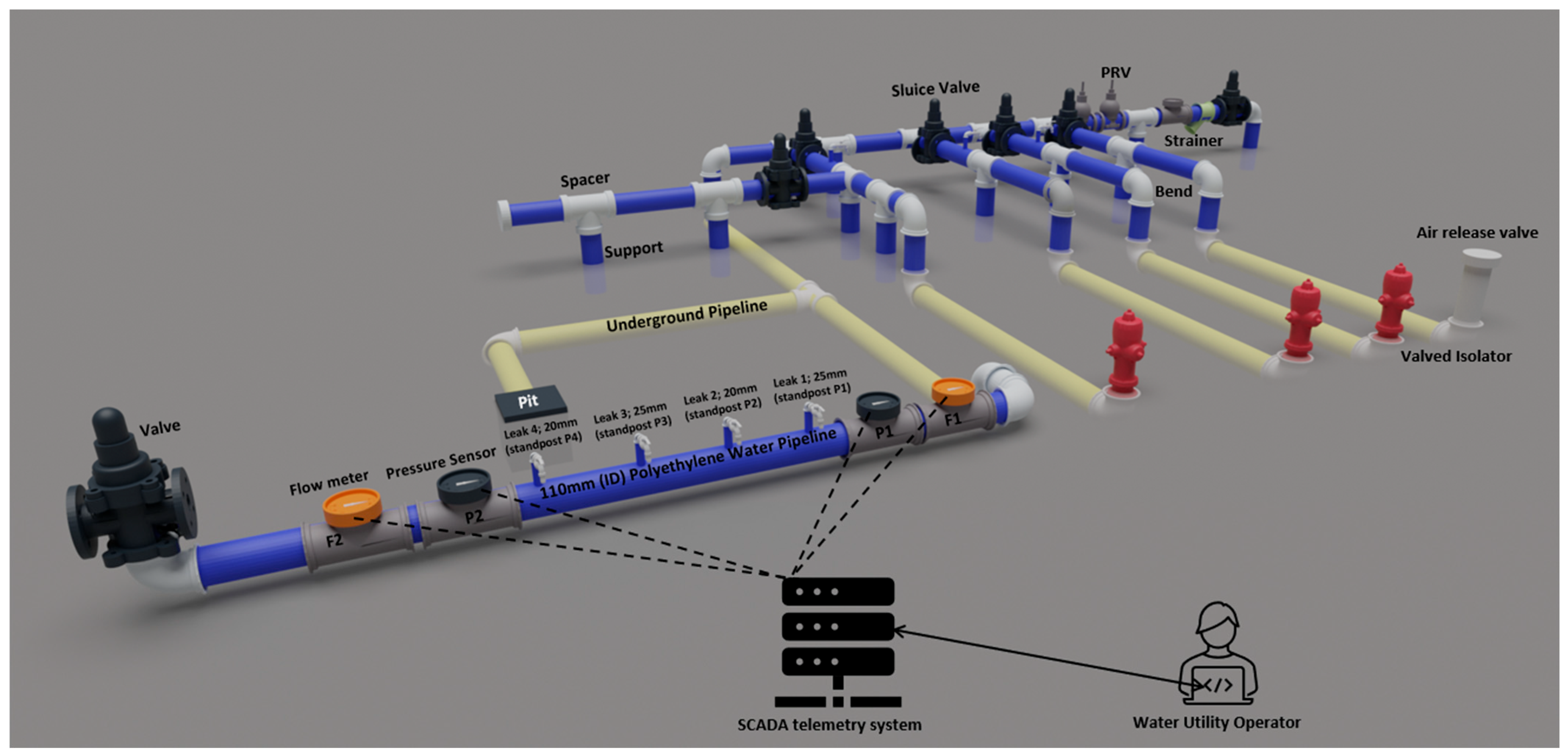
An experimental prototype water supply system setup is located in Melton, Victoria, Australia as shown in Figure 1, which is developed at the training yard of a local water utility. Figure 2 shows the detailed diagram of the experimental water system setup at Melton.

A 110 mm internal diameter, 110 m length polyethylene pipe was equipped with two flow meters and two pressure sensors. The pipe is connected to a 100 mm water pipeline. Leaks were simulated using various pipe outlets of sizes 20 mm and 25 mm from 110 mm pipe (Figure 2). The flow meters and pressure sensors were integrated into a SCADA wireless system to monitor and record the experimental data. In Figure 2, the inlet flow meter is F1, the outlet flow meter is F2, the inlet pressure sensor is P1, and the outlet pressure sensor is P2.

The study integrates the key parameters such as flow rate, pressure variations, addition of the change in pressure, and flow variations as pressure and flow acceleration, respectively. Timestamp data are also included to establish a detailed understanding of the pipeline dynamics under different operating conditions, and finally, the best performance models are found based on the data collected, which are then used to detect leaks and bursts in the water pipeline.

• Instruments Used:

(a) 

Pressure Transducer

A pressure transducer (Model: MX232, Measurex Pty Ltd., Melbourne, Australia; Serial No: 3115262003) was employed to monitor pressure within the pipeline system. The device features a measurement range of 0–16 bar and a manufacturer-specified accuracy of ±0.25% of Full Scale (FS). It was installed using PTFE thread sealing and securely interfaced with the data acquisition system to ensure reliable measurements. The sensor was factory calibrated prior to installation, and functional validation was conducted through comparison with a certified reference pressure gauge. The observed measurement deviations remained within the stated accuracy range, thereby confirming the sensor’s reliability under field conditions.

(b) 

Pressure Transmitter

In addition to the pressure transducer, an ABB 261GSU SMART pressure transmitter (Type: 261GSU/VT1/N21) was utilised for high-precision pressure monitoring. The instrument is equipped with a silicon oil-filled Hastelloy C276 diaphragm and has a configurable measurement span of 150 kPa. The manufacturers are ABB Ltd., Zürich, Switzerland. Operating on a 4–20 mA loop-powered output with a supply voltage range of 10.5–32 V DC. According to the manufacturer’s specifications, the device offers a standard accuracy of ±0.1% of span, with an optional high-accuracy mode of up to ±0.04% of span. Prior to deployment, the transmitter underwent comprehensive field calibration using a certified pressure calibrator traceable to NIST standards.

(c) 

Mechanical Flow Meter

A volumetric multijet dry dial water meter (Serial No: 2404013684), compliant with International Organization for Standardization (ISO) 4064 standards [23], was used to measure volumetric flow during the experiment. The ISO organisation is based in Geneva, Switzerland. The manufacturer is Zenner International GmbH & Co. KG, Saarbrücken, Germany. The device is equipped with a pulse output to facilitate continuous data logging. It provides an accuracy of ±2% for flow rates above the transitional threshold and ±5% below it. The meter was delivered factory-calibrated and accompanied by a compliance certificate. It was installed with tamper-proof sealing to maintain data integrity. A preliminary verification test was conducted to confirm operational performance and the consistency of the pulse signal under test conditions.

(d) 

Electromagnetic Flow Meter

To complement the mechanical measurements, a Siemens SITRANS F M MAG 8000 electromagnetic flow meter was deployed for continuous volumetric flow monitoring. The manufacturer is Siemens AG, Munich, Germany. This battery-powered inline device is factory-calibrated to ISO/IEC 17025 standards [24] and provides a measurement accuracy of ±0.4% of the actual flow rate. For enhanced accuracy, certain model variants support precision up to ±0.2%. The meter incorporates SENSORPROM™ technology, which ensures the preservation of calibration and configuration data across installations. The device was deployed in its original calibrated state. Real-time flow data were retrieved via the onboard display and transmitted through either pulse output or an integrated SCADA telemetry system. The SCADA data were recorded at a fixed interval of one minute, corresponding to a sampling time of 60 s and a sampling frequency of 0.0167 Hz.

Mechanical flow meters were used to check the flow from four leaks as shown in Figure 2. Electromagnetic flow meters were used to measure flow at F1 and F2. Pressure transducers were used to measure pressure P1 and P2, and a pressure transmitter was used to validate the pressure transducers.

3. Feature Engineering of the Collected Data from the Experimental Site

The data collected from the experimental setup, combining various scenarios of outlet flow(s), were used to train various supervised machine learning models, with the objective of identifying the most effective model for early leak detection. The data from the flow meters and the pressure sensors from the SCADA of the Melton experimental setup are shown below in

Table 1. SCADA data from flow meters and pressure sensors.

Timestamp	Flow F1 (L/s)	Pressure P1 (kPa)	Flow F2 (L/s)	Pressure P2 (kPa)
4/07/2024 11:15:20	12.87	165	12.17	140
4/07/2024 11:25:00	14.35	168	11.87	142
4/07/2024 11:46:10	15.20	155	12.71	132
4/07/2024 12:03:50	11.34	170	11.33	143
5/07/2024 15:45:00	8.27	43	6.89	41
11/07/2024 11:08:00	12.38	157	10.88	139
12/07/2024 11:05:00	12.48	128	12.32	106
16/07/2024 12:52:00	13.85	136	12.83	108
23/07/2024 14:07:00	15.07	160	13.98	131
23/07/2024 14:43:00	13.45	125	12.77	104
30/07/2024 14:24:00	13.66	154	13.94	125
30/07/2024 14:37:00	16.27	118	12.56	92
6/08/2024 11:31:00	11.06	87	10.77	77
6/08/2024 12:52:00	14.34	128	12.56	106

.

The classification of the leak and burst detection system consists of three distinct categories, which are shown in

Table 2. Leak classifications and leak types.

Leak Classifications	Leak Type
0	No leak
1	Minor leak
2	Major leak

and described below:

• Class 0 (No Leak): This category represents normal operational conditions where no anomalies in pressure, flow, or sensor readings indicate the presence of a leak. The system operates optimally without any water loss or disruptions.
• Class 1 (Minor Leak): This classification indicates the presence of a small leak within the pipeline network. Minor leaks are often characterised by slight reductions in pressure and minimal deviations in sensor data, which may not significantly impact system performance but can lead to cumulative water losses over time if left unaddressed.
• Class 2 (Major Leak): This category represents severe leakages that pose an immediate risk to the water distribution system. Major leaks typically result in significant pressure drops, abnormal flow variations, and substantial water loss, requiring urgent intervention to prevent infrastructure damage and service disruptions.

This classification scheme provides a structured approach to automating leak detection models by enabling machine learning algorithms to differentiate between normal and faulty conditions. The precise identification of leak severity allows for real-time monitoring, predictive maintenance, and efficient resource allocation in water management systems.

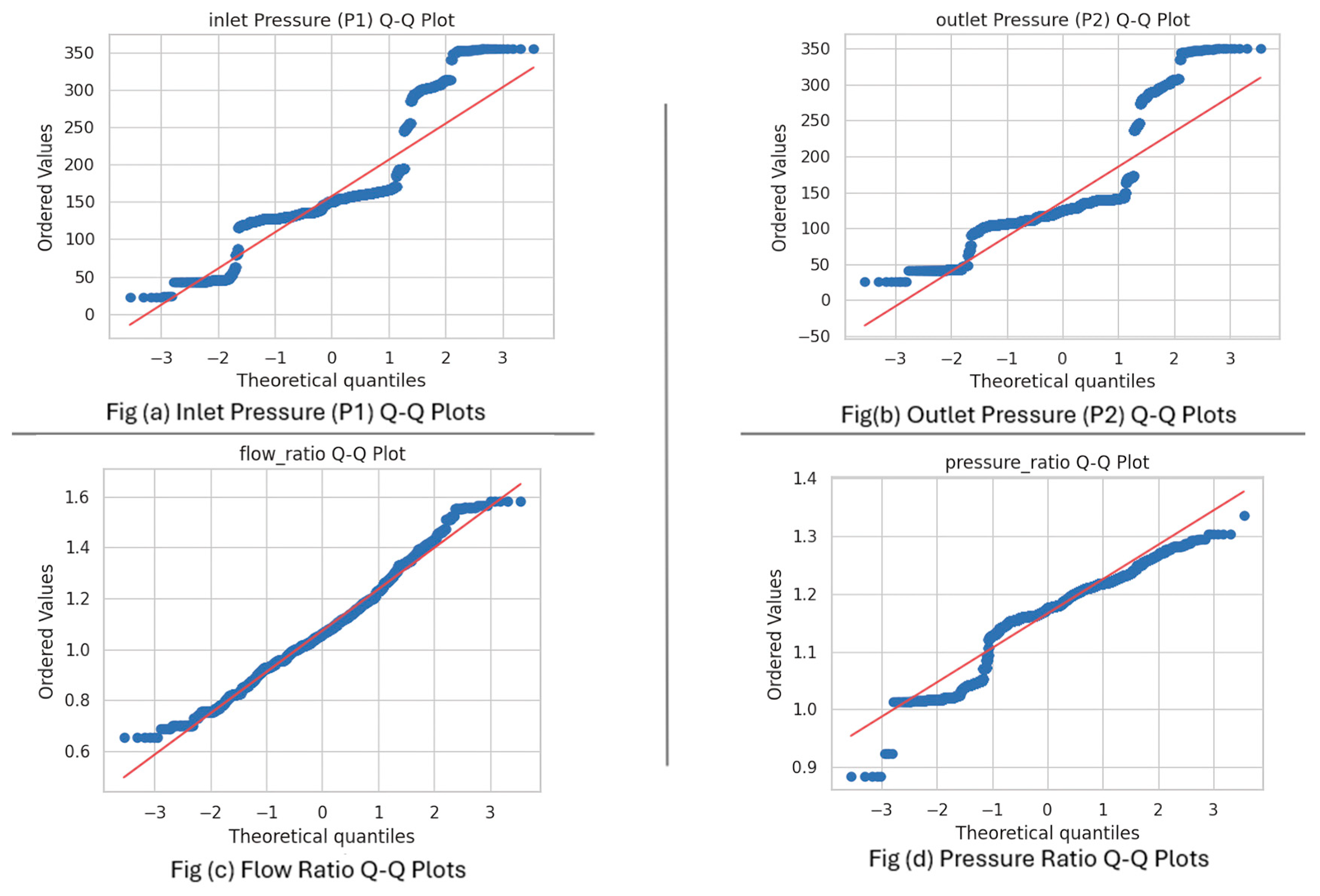
Quantile–quantile (Q–Q) plots were employed to assess the normality of the inlet pressure, outlet pressure, flow ratio, and pressure ratio distributions for the collected data (Figure 3). In these plots, the x-axis represents the theoretical quantiles assuming a standard normal distribution, while the y-axis displays the ordered values of the observed data. The flow ratio, as depicted in its Q–Q plot, likely represents a normalised measure of flow within the system, potentially the ratio of flow rates at different locations or relative to a baseline. Similarly, the pressure ratio signifies a normalised pressure measure, possibly the ratio of pressures at different points or relative to a reference pressure. Deviations of the plotted points from the diagonal red line indicate departures from a normal distribution, providing visual diagnostics critical for anomaly detection, model validation, and understanding system performance under varying conditions. Figure 3 presents the Q–Q plots for the considered parameters. For the inlet pressure (P1) and outlet pressure (P2) (Figure 3a,b), the data points generally align along the diagonal, suggesting approximate normality with minor deviations at the distribution tails, corresponding to unusual events or fluctuations in the pipeline system. For the flow ratio and pressure ratio (Figure 3c,d), a similar linear trend is observed, although some deviations are present. These deviations are essential for identifying anomalies in flow and pressure relationships, which are critical indicators of leaks or bursts. Overall, the proximity of the plot points to the normal line supports the generalisability and robustness of the modelling approach employed in this project.

$$R^2=1-{\displaystyle \frac{{\sum }_{i=1}^n{\left(y_i-\widehat{y_i}\right)}^2}{{\sum }_{i=1}^n{\left(y_i-\overline{y}\right)}^2}}$$

(1)

where

$R^2$—Coefficient of determination—measures how well the observed outcomes are replicated by the model (in this case, how well the data follows a normal distribution in a Q–Q plot).

$y_i-$ Observed value (the actual data point from your dataset).

$\widehat{y_i}$—Predicted value (the value on the reference line in the Q–Q plot, corresponding to a perfect normal distribution).

$\overline{y}$—Mean of the observed values.

$n$—Total number of observations.

The numerator ${\sum }_{i=1}^n{\left(y_i-\widehat{y_i}\right)}^2$ represents the sum of squares of residuals (how far each data point deviates from the expected normal value).

The denominator ${\sum }_{i=1}^n{\left(y_i-\overline{y}\right)}^2$ represents the sum of squares of residuals (how far each data point deviates from the expected normal value).

Thus $R^2$, indicates the proportion of variance explained by the model. A value close to 1 suggests a good fit to the normal distribution.

The R² values obtained from the Q–Q plots for each graph are as follows: Figure 3a—inlet pressure as 0.7556, Figure 3b—outlet pressure as 0.7071, Figure 3c—flow ratio as 0.9888, and Figure 3d—pressure ratio as 0.9019. These results show that flow ratio and pressure ratio follow a normal distribution quite closely, with very few anomalies. On the other hand, the lower R² values for inlet and outlet pressure suggest some deviations from normality, which could be a sign of anomalies or unusual behaviour in the pressure data.

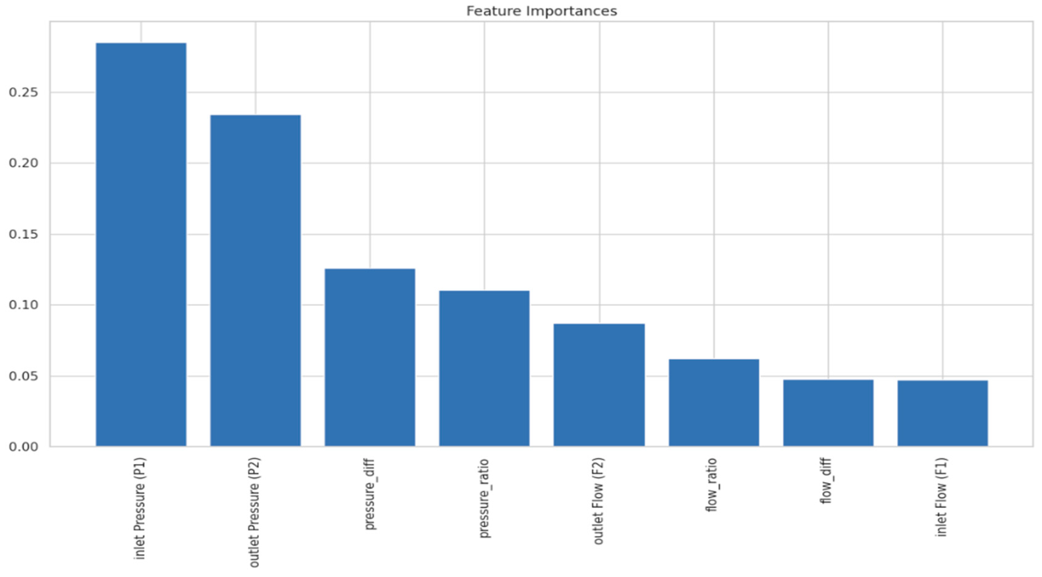
Figure 4 highlights the feature importance graph of inlet pressure (P1), which is the most critical leak/burst predictor, followed by outlet pressure (P2) and pressure difference. Prioritising the real-time monitoring of these parameters can significantly enhance early warning capabilities. To improve system reliability, sensor placement should be optimised, particularly at inlet and outlet locations, while hydraulic models should be refined to better capture pressure dynamics. Additionally, implementing threshold-based alarms for pressure deviations and directing maintenance efforts to regions with frequent anomalies can further strengthen leak detection and overall pipeline integrity.

4. Methodology for the Detection of Leaks and Bursts in Water Pipelines

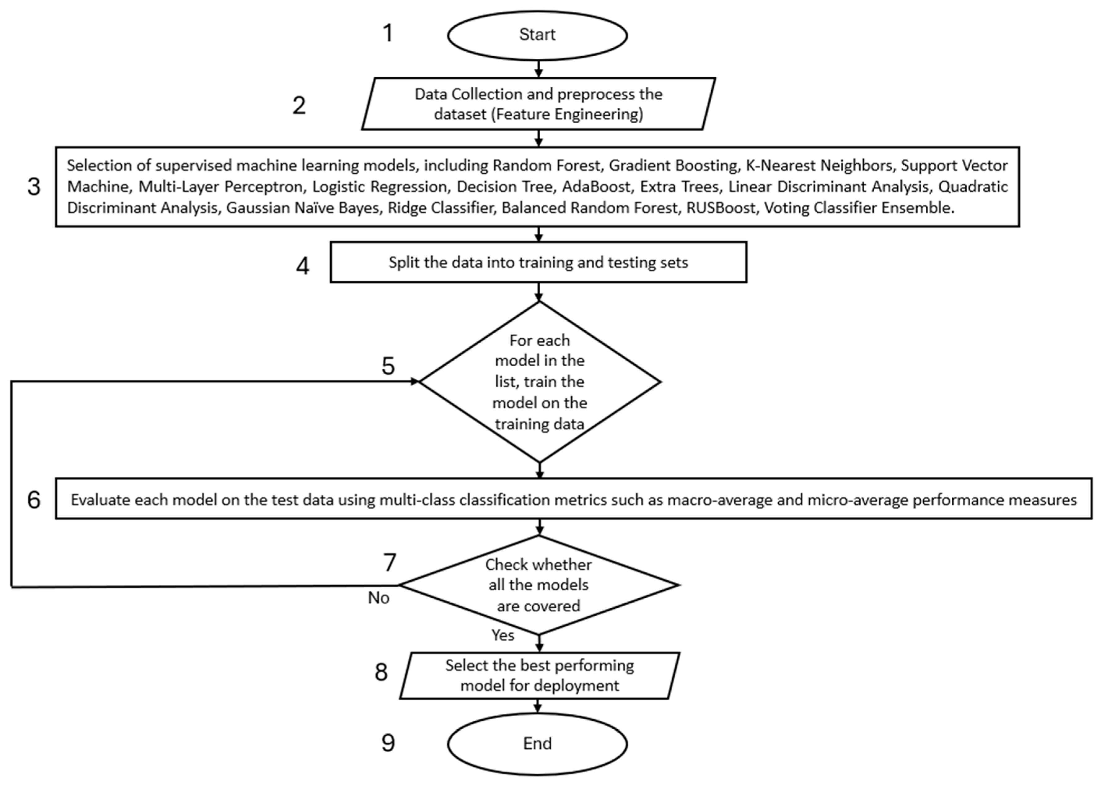
Figure 5 below shows the flow chart for the selection of the model with the best performance. The flowchart illustrates the process of selecting and validating a machine learning model for detecting leaks and bursts in water pipelines. The stages of the methodology are depicted in Figure 5, and the detailed explanations of each step are provided below:

• Start

This step initiates the process to identify suitable machine learning models for final selection.

2.

Data Collection and Preprocessing (Feature Engineering)

In this stage, data is gathered from the SCADA and prepared for analysis. Preprocessing includes handling missing values, encoding categorical variables, normalizing numerical features, and performing feature selection or extraction. Proper preprocessing ensures the quality and integrity of the data, which is critical for model performance.

3.

Model Selection

A diverse set of 14 supervised machine learning algorithms is selected for comparison. The selection of these models was based on their historical performance in similar leak detection tasks as outlined in the Introduction, covering a wide spectrum of classification types—tree-based, ensemble, kernel-based, and probabilistic. This ensures a broad benchmarking across simple and complex classifiers. While hybrid models like SVM combined with Random Forest (SVM-RF) have shown promise in prior studies (e.g., [12]), they were not included in this phase due to computational overhead and complexity in parameter tuning, which are not ideal for real-time field deployment. However, individual performances of SVM and RF were tested separately to gauge their standalone efficacy, as a prerequisite for future ensemble or hybrid development. These include ensemble methods (Random Forest, AdaBoost, RUSBoost, Voting Classifier Ensemble), distance-based methods (K-Nearest Neighbours), linear models (Logistic Regression, Ridge Classifier), tree-based models (Decision Tree), probabilistic models (Gaussian Naïve Bayes), discriminant analysis methods (Linear Discriminant Analysis, Quadratic Discriminant Analysis), neural networks (Multi-Layer Perceptron), and kernel-based methods (Support Vector Machine). The purpose is to assess a wide range of models to identify the most suitable one for the task.

4.

Split the Data into Training and Testing Sets

The dataset is divided into training and testing subsets, typically in a ratio such as 80:20. The training set is used to fit the models, while the testing set is reserved for evaluating their performance. This step ensures that the models are assessed on unseen data, helping to evaluate their generalisation capabilities.

5.

Model Training

Each selected machine learning model is trained using the training data. During this process, the algorithm learns patterns in the data and adjusts its internal parameters to minimize classification errors. The outcome is a set of trained models ready for evaluation.

6.

Model Evaluation

The models were evaluated using the following equations:

Precision = TP/(TP + FP)
Recall = TP/(TP + FN)
F1-Score = 2 × (Precision × Recall)/(Precision + Recall)
Accuracy = (TP + TN)/(TP + TN + FP + FN)

where TP = true positives, FP = false positives, FN = false negatives, and TN = true negatives. True positives (TP) are correctly predicted leak events, false positives (FP) are incorrectly predicted leaks where there are none, false negatives (FN) are missed actual leaks, and true negatives (TN) are correctly identified non-leak events.

The macro-average computes metrics independently for each class and takes the unweighted mean, treating all classes equally. The micro-average aggregates contributions from all classes to compute the average metric, favouring classes with more samples. These metrics were selected to evaluate the models’ ability to distinguish between the three classes (no leak, minor leak, and major leak), even in imbalanced datasets. The F1-score, in particular, balances precision and recall, which is critical in leak detection tasks where both false negatives (missed leaks) and false positives (false alarms) have operational consequences. The dataset was constructed to maintain an approximately balanced distribution across the three classes (no leak, minor leak, and major leak). This design was intentional to minimise bias and ensure fair model comparison. However, we recognise that in real-world data, no-leak conditions are more frequent. To address this, future research will explore class imbalance mitigation strategies such as SMOTE (Synthetic Minority Oversampling Technique) and cost-sensitive learning.

The trained models are evaluated on the testing dataset using multi-class classification performance metrics. These include macro-average and micro-average measures of precision, recall, and F1-score. Macro-average calculates metrics independently for each class and then averages them, while micro-average aggregates contributions of all classes. This ensures a comprehensive evaluation of model performance, especially in imbalanced datasets.

7.

Check if all the models are covered

At this stage, the model will check if all the models considered have been evaluated. If Yes go to step 8 otherwise go to step 5.

8.

Model Selection for Deployment

Based on the evaluation results, the best-performing model is selected for deployment. The selection criteria may include accuracy, macro- and micro-averaged precision, recall, F1-score, and robustness across classes. This step ensures that the deployed model is both effective and reliable.

9.

End

This final step concludes the model development pipeline. The result is a validated, high-performing classification model ready for deployment in a production environment or for further use in predictive applications.

The classification performance of each model was assessed using standard evaluation metrics. Precision measures the proportion of correctly predicted positive instances out of all predicted positives, while recall quantifies the model’s ability to correctly identify all relevant instances. The F1-score represents the harmonic mean of precision and recall, ensuring a balanced evaluation of the model’s predictive power. Macro averaging computes the unweighted mean of precision, recall, and F1-score across all classes, treating each class equally. Conversely, weighted averaging accounts for class imbalances by weighting the contributions of each class based on the number of instances present. Finally, accuracy denotes the overall proportion of correctly classified instances in the dataset.

The dataset was constructed to maintain an approximately balanced distribution across the three classes (no leak, minor leak, and major leak). This design was intentional to minimise bias and ensure fair model comparison. However, we recognise that in real-world data, no-leak conditions are more frequent. To address this, future research will explore class imbalance mitigation strategies such as SMOTE (Synthetic Minority Oversampling Technique) and cost-sensitive learning.

5. Results

Multi-class classification plays a crucial role in machine learning applications where the objective is to categorise input data into three or more classes. The evaluation of classification models relies on performance metrics such as precision, recall, F1-score, macro and weighted averages, and accuracy. In this study, 14 different classification models were assessed and systematically compared to identify the most suitable models for leak and burst detection in water distribution systems. The performance of these models was rigorously evaluated, and the optimal model was selected based on its accuracy and reliability. The outcome of this research contributes to the development of an advanced integrated software-hardware-based system for real-time leak detection in water distribution networks, offering potential improvements in water conservation and infrastructure management.

5.1. Performance Evaluation of Multi-Class Classification Models for Leak and Burst Detection

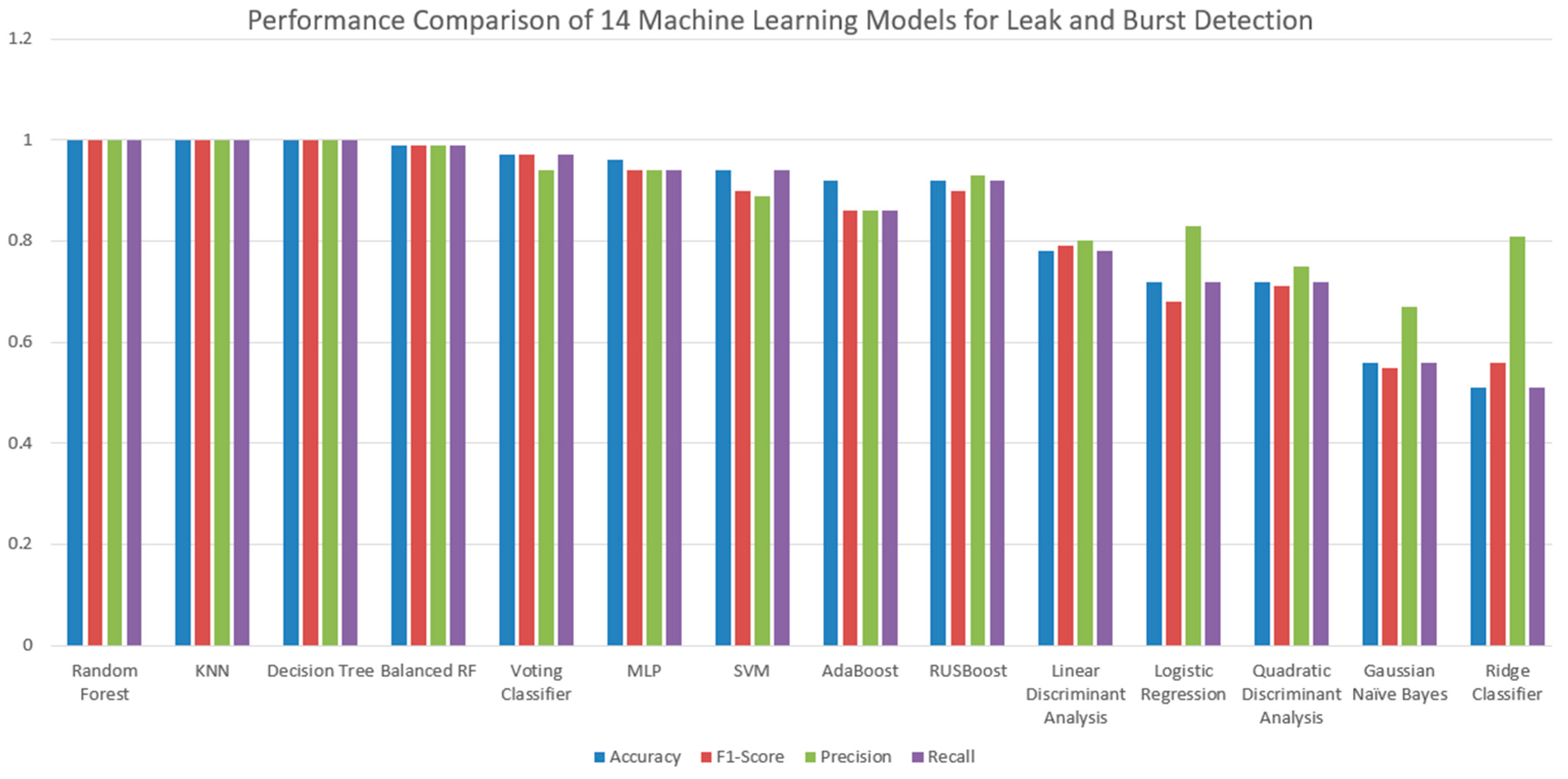
Figure 6 (below) presents a comparative analysis of supervised machine learning models for leak detection in water pipelines, evaluated through multi-class classification.

Table 3. Comparative performance of multi-class classification models for leak detection in water pipelines.

Model Name	Class 0 Precision	Class 0 Recall	Class 0 F1-Score	Class 1 Precision	Class 1 Recall	Class 1 F1-Score	Class 2 Precision	Class 2 Recall	Class 2 F1-Score	Macro Average Precision	Macro Average Recall	Macro Average F1-Score	Weighted Average Precision	Weighted Average Recall	Weighted Average F1-Score	Accuracy F1-Score
Random Forest	1	1	1	1	1	1	1	1	1	1	1	1	1	1	1	1
K-Nearest Neighbours	1	1	1	1	1	1	1	1	1	1	1	1	1	1	1	1
Support Vector Machine	1	0.99	1	0.7	1	0.82	0.98	0.82	0.90	0.89	0.94	0.90	0.95	0.94	0.94	0.94
Multi-Layer Perceptron	1	0.99	1	0.88	0.89	0.88	0.94	0.95	0.95	0.94	0.94	0.94	0.96	0.96	0.96	0.96
Logistic Regression	0.98	0.75	0.85	0.35	0.82	0.49	0.80	0.65	0.71	0.71	0.74	0.68	0.83	0.72	0.75	0.72
Decision Tree	1	1	1	1	1	1	1	1	1	1	1	1	1	1	1	1
AdaBoost	0.99	0.98	0.98	0.73	0.70	0.72	0.88	0.91	0.89	0.86	0.86	0.86	0.92	0.92	0.92	0.92
Linear Discriminant Analysis	0.91	0.84	0.88	0.45	0.58	0.51	0.78	0.78	0.78	0.71	0.73	0.72	0.80	0.78	0.79	0.78
Quadratic Discriminant Analysis	0.83	0.91	0.87	0.38	0.66	0.49	0.79	0.44	0.56	0.67	0.67	0.64	0.75	0.72	0.71	0.72
Gaussian Naïve Bayes	0.91	0.44	0.59	0.22	0.20	0.21	0.49	0.89	0.63	0.54	0.51	0.48	0.67	0.56	0.55	0.56
Ridge Classifier	0.99	0.40	0.57	0.22	0.88	0.35	0.77	0.53	0.62	0.66	0.60	0.51	0.81	0.51	0.56	0.51
Balanced Random Forest	1	0.99	1	0.98	1	0.99	0.99	0.99	0.99	0.99	0.99	0.99	0.99	0.99	0.99	0.99
RUSBoost	0.97	0.99	0.98	1	0.43	0.60	0.83	0.99	0.90	0.93	0.80	0.83	0.93	0.92	0.90	0.92
Voting Classifier Ensemble	1	0.99	1	0.82	1	0.90	0.99	0.91	0.95	0.94	0.97	0.95	0.97	0.97	0.97	0.97

summarises the comparative performance of fourteen machine learning models. The performance evaluation revealed that several ensemble-based and distance-based classifiers achieved remarkably high levels of predictive accuracy across all classes. Specifically, the K-Nearest Neighbours (KNN), Random Forest, and Decision Tree models reported perfect scores (1.00) for precision, recall, and F1-score across all three classes, as well as macro and weighted averages, culminating in an overall accuracy of 1.00. This performance with accuracy of 1.00 in this case can be attributed to several key factors in our controlled experimental setup and dataset construction, including balanced and clearly separated classes, well-engineered and distinctive features, low-noise and tightly controlled conditions, and equal temporal sampling with consistent event durations.

5.1.1. Model Performance Comparisons:

In contrast, other models exhibited varied performances. Support Vector Machine (SVM) and Multi-Layer Perceptron (MLP) achieved strong but not perfect accuracies of 0.94 and 0.96, respectively, indicating potential sensitivity to parameter tuning and class boundaries. The AdaBoost model performed reasonably well with an accuracy of 0.92, although slightly lower precision and recall in some classes suggest vulnerability to noise or class imbalance. Models based on linear assumptions, such as Logistic Regression, Linear Discriminant Analysis (LDA), and Quadratic Discriminant Analysis (QDA), demonstrated moderate performance, with accuracies ranging from 0.72 to 0.78, likely due to mismatches between model assumptions and the dataset’s underlying structure. Gaussian Naïve Bayes and Ridge Classifier performed comparatively poorly, achieving accuracies of 0.56 and 0.51, respectively, reflecting limitations related to their simplifying assumptions, such as feature independence or regularization constraints. Notably, ensemble variants such as Balanced Random Forest and Voting Classifier Ensemble achieved very high accuracies of 0.99 and 0.97, respectively, further validating the robustness of ensemble learning techniques. Overall, these findings affirm that ensemble learning, by combining bias reduction and variance control strategies, consistently outperforms traditional and linear classifiers across multiple evaluation metrics. The selection of the most effective models was based on their predictive performance across multiple evaluation criteria.

Top Performing Models

The analysis indicates that tree-based classifiers, including KNN, Random Forest, Decision Tree, and Balanced Random Forest, achieved near-optimal classification performance. These models demonstrated consistently high precision, recall, and F1-scores (≈1.00), signifying their superior learning capabilities and generalisation across different classes. The robust nature of these models, particularly in handling imbalanced and complex feature distributions, makes them highly suitable for leak and burst detection.

Moderate Performing Models

Models such as the Support Vector Machine (SVM), Multi-Layer Perceptron (MLP), AdaBoost, and Voting Classifier Ensemble exhibited competitive classification capabilities, albeit with slightly reduced recall scores for certain classes. These models achieved macro and weighted F1-scores ranging from 0.90 to 0.97, indicating reliable predictive performance. However, their slightly lower recall values suggest a marginally higher rate of false negatives, which could be detrimental in critical water distribution monitoring scenarios.

Weak Performing Models

Traditional probabilistic and linear classifiers, including Gaussian Naïve Bayes, Quadratic Discriminant Analysis (QDA), and Ridge Classifier, demonstrated comparatively lower classification accuracy. Gaussian Naïve Bayes suffered from high variance in precision (0.22–0.91) and F1-scores (0.21–0.63), primarily due to its assumption of feature independence. Similarly, QDA and Ridge Classifier exhibited macro F1-scores below 0.70, indicating their limitations in effectively capturing complex decision boundaries in the dataset. Given the critical nature of leak and burst detection, where misclassification can result in severe operational consequences, these models were deemed unsuitable for deployment in real-world scenarios.

The above graphical comparison highlights that Random Forest, KNN, and Decision Tree models consistently outperform others across all performance metrics, making them ideal candidates for leak and burst detection in water distribution systems. Ensemble methods such as Balanced Random Forest and RUSBoost also show strong potential. In contrast, linear and probabilistic models underperform, likely due to their limited ability to capture complex patterns in the dataset. This confirms that tree-based and ensemble models offer the most robust solutions under the experimental conditions used.

6. Leak and Burst Detection Validation on the Selected Models

Some leak and burst detection conditions based on the ML outputs are provided in

Table 4. Leak and burst detection conditions of the experimental water system.

Algorithm Used	Timestamp	Flow (F1)	Pressure (P1)	Flow (F2)	Pressure (P2)	Flow Diff.	Pressure Diff.	Flow Ratio	Pressure Ratio	Flow Gradient	Pressure Gradient	Flow Acceleration	Pressure Acceleration	Leak Type	Leak Type Predicted
No leak data	7/4/24 11:15	0.56	0.42	0.61	0.35	0.66	0.2	0.57	0.26	0.51	0.42	0.51	0.42	0	0
K-Nearest Neighbor Minor leak	7/11/24 11:57	0.68	0.41	0.54	0.35	0.34	0.37	0.26	0.34	0.52	0.42	0.52	0.42	1	1
K-Nearest Neighbor Major leak	7/8/24 15:37	0.37	0.68	0.38	0.66	0.65	0.68	0.52	0.57	0.52	0.42	0.52	0.42	2	2
Decision Tree Major leak	8/6/24 15:25	0.57	0.32	0.66	0.25	0.72	0.2	0.64	0.21	0.52	0.42	0.52	0.42	2	2
Decision Tree Minor leak	8/6/24 12:37	0.79	0.30	0.54	0.23	0.14	0.28	0.12	0.19	0.53	0.42	0.53	0.42	1	1
Random Forest Minor leak	7/11/24 10:36	0.69	0.41	0.62	0.35	0.46	0.34	0.38	0.33	0.52	0.34	0.52	0.34	1	1
Random Forest Major leak	7/8/24 15:03	0.65	0.68	0.36	0.66	0.12	0.62	0.02	0.55	0.52	0.42	0.52	0.42	2	2

.

7. Conclusions

The results suggest that machine learning techniques, particularly KNN, Random Forest and Decision Tree, are the most effective models for leak and burst detection for the data collected for a prototype water system. Their ability to capture complex patterns, adapt to non-linear decision boundaries, and handle imbalanced datasets ensures their reliability in detecting leaks and bursts with high accuracy.

In contrast, linear models such as Logistic Regression and Ridge Classifier failed to capture the intricate relationships within the dataset, making them less effective. Similarly, the performance of Gaussian Naïve Bayes was significantly affected by the assumption of feature independence, leading to high classification errors.

This research highlights the effectiveness of machine learning approaches in multi-class classification for leak and burst detection. The selected models are Random Forest, Decision Tree, and KNN. These models demonstrated superior predictive performance and robustness. Their high precision and recall values indicate their ability to minimise false negatives, which is crucial for early detection and prevention of leaks and bursts in water distribution systems. While the results demonstrate excellent classification performance, it is important to acknowledge the potential for overfitting due to the use of a controlled and relatively noise-free dataset. Future work will include testing on field data and incorporating stochastic noise to validate model robustness.

8. Future Recommendations

Future research should explore optimising the machine learning models by incorporating more advanced data sources, such as real-time sensor data from IoT devices, including SCADA, Kingfisher, historian, and high-frequency measurements. It can involve optimising these models further by integrating feature engineering techniques, sensor-based real-time data collection, and hybrid ensemble approaches to enhance detection capabilities in dynamic water distribution environments. Future studies should incorporate sensitivity analyses to assess model performance under conditions of sensor noise, missing data, and calibration errors. This will provide deeper insights into model resilience and inform strategies for fault-tolerant deployment. Additionally, investigating the impact of different pipeline materials, diameters, and environmental conditions on leak detection accuracy could enhance model generalisability. This would further improve the efficiency and sustainability of water resource management.