1. Introduction
Freshwater quality has become a growing concern globally due to the increasing levels of contamination from domestic sewage, industrial discharge, agricultural runoff, and urban development [
1,
2]. Rivers, which serve as a critical water source for human consumption, agriculture, and industry, are particularly vulnerable to such pollution, especially in developing countries like India [
3,
4,
5,
6,
7]. Maintaining healthy river ecosystems is not only essential for public health and environmental balance but also directly contributes to achieving multiple United Nations Sustainable Development Goals (SDGs), including clean water and sanitation (SDG 6) and good health and well-being (SDG 3) [
8,
9,
10,
11]. One of the widely used approaches to summarize and communicate the status of water bodies is the Water Quality Index (WQI), which consolidates multiple physicochemical and microbial parameters into a single numeric score or qualitative category, such as Excellent, Good, Medium, or Poor. Traditionally, the WQI is computed using a manual method involving weighted averages of selected parameters followed by classification rules [
12,
13,
14,
15,
16,
17,
18]. While effective in summarizing complex data, this process is time consuming, dependent on fixed thresholds, and lacks flexibility for real-time or large-scale implementation. Additionally, manual computation may not capture nonlinear relationships among indicators or detect subtle shifts in water quality, which are critical for early warning and timely interventions [
19,
20,
21,
22]. In this context, machine learning (ML) offers a promising alternative for predictive and automated water quality assessment. ML models are capable of handling large, multidimensional datasets, learning complex patterns, and producing accurate predictions with minimal human interference [
23,
24,
25,
26,
27]. Although there is a growing body of literature exploring ML applications in environmental monitoring, most existing studies are limited in scope—focusing on either classification or regression, but not both, using only physicochemical parameters while ignoring microbial indicators, or omitting model interpretability and spatial variability altogether [
28,
29,
30]. Furthermore, many models are built in isolation from policy-relevant outputs, thereby limiting their real-world applicability.
Addressing these limitations, the present study proposes an integrated ML-based framework to model, predict, and classify Water Quality Index using a curated dataset of river water samples from India. The dataset includes eight essential indicators—Temperature, pH, Dissolved Oxygen, Biological Oxygen Demand, Conductivity, Nitrate/Nitrite, Fecal Coliform, and Total Coliform—offering a comprehensive representation of both chemical and microbial water quality dimensions. The WQI was calculated using standard weight-based methodology and used as the target variable for supervised learning. A dual modeling pipeline was employed; regression models such as Linear Regression, Random Forest Regressor, and Gradient Boosting Regressor were used to predict continuous WQI values, while classification models including Logistic Regression, Random Forest Classifier, and Gradient Boosting Classifier were used to categorize water quality into classes. Each model was evaluated using appropriate performance metrics like RMSE, MAE, R2 for regression, and Accuracy, Precision, Recall, and F1-Score for classification.
Additionally, the study incorporated Exploratory Data Analysis (EDA) to visualize trends and parameter distributions, and spatial mapping to understand geographic variability in water quality. Feature importance analyses—using Gini impurity and permutation-based techniques—were conducted to interpret model decisions and identify the most influential parameters. Residual plots and misclassification analysis further helped assess model reliability and generalization. The results showed over 95% agreement between ML-predicted WQI classes and manually computed ones, confirming the reliability of the proposed approach. Unlike prior studies, this work offers a unified framework that combines prediction, classification, interpretability, and spatial analysis in one coherent system.
The novelty of the study lies in its integration of chemical and microbial indicators, dual-modeling approach, explainable AI features, and scalable design suitable for real-time water quality monitoring and policy guidance. Overall, the framework demonstrates the potential of machine learning to transform traditional environmental monitoring into a more automated, interpretable, and scalable process that can support data-driven decision-making in water resource management.
2. Methodology
This section outlines the comprehensive methodological framework adopted to predict and classify the Water Quality Index (WQI) using supervised machine learning. The approach integrates regression and classification modeling, feature explainability, misclassification analysis, and comparison with rule-based classification. Additionally, geospatial mapping of input features provides a spatial context to the data and supports interpretation of regional trends. The methodology was implemented in a modular pipeline to ensure the reproducibility, scalability, and robustness across the various stages of the analysis.
2.1. Dataset Description and Preparation
Effective modeling of the Water Quality Index (WQI) requires a well-structured dataset that captures both the physicochemical characteristics of water bodies, and any environmental indicators derived. The current study utilizes a tabular dataset extracted from the “Open Government Data (OGD) Platform India” (
https://www.data.gov.in) comprising multi-parameter observations from river monitoring stations, which are processed and enriched through various stages before model training. This section outlines the dataset source, transformation pipeline, and the final preprocessed features used for machine learning tasks.
This dataset was selected for its national coverage, inclusion of eight validated water quality parameters, and open accessibility via a government portal. Despite a moderate sample size (442 records after cleaning), the data offers sufficient spatial and feature diversity for machine learning tasks, especially with ensemble models known to perform well on structured, mid-sized datasets.
2.2. Source and Description of Raw Dataset
Building on the dataset overview, the raw observations were obtained from routine monitoring of river water quality across various Indian states, including locations such as Godavari at Jayakwadi Dam and Someshwar Temple. The observations encompass parameters like Temperature (°C), Dissolved Oxygen (DO), Biochemical Oxygen Demand (BOD), pH, Conductivity, Nitrate/Nitrite concentration, and Coliform counts (Fecal and Total). Each sample is associated with metadata such as station code, location, and state. In total, the dataset spans 534 records with substantial spatial diversity. These parameters form the basis for WQI computation and ML-based modeling.
Each observation in the dataset was associated with a timestamp representing the sampling date. However, the sampling frequency was not uniform across all stations or states. While many sites reported data monthly, others followed quarterly or irregular sampling intervals, depending on their operational protocols. This variability was noted and accounted for during the data preprocessing phase, but the study focuses on spatial rather than temporal trends due to these inconsistencies.
2.3. Computation of the Water Quality Index (WQI)
The Water Quality Index was computed using the Weighted Arithmetic Index Method, which standardizes each parameter into a unit-less sub-index (SI) based on its observed value and environmental standards. The parameters considered in this computation included pH, Dissolved Oxygen (DO), Biological Oxygen Demand (BOD), Conductivity, Nitrate/Nitrite concentration, Fecal Coliform, and Total Coliform. For each parameter
, a sub-index
was calculated using a predefined empirical formula that transforms raw observations into a 0–100 quality scale. Each SI was then multiplied by a weight wiw_iwi, representing the relative importance of that parameter in assessing water quality, as prescribed by the national environmental standards provided by the Central Pollution Control Board (CPCB), Government of India [
30]. The overall WQI was computed using the following formula:
All sub-index computations and aggregations were implemented programmatically using Python to ensure consistency and scalability. Special care was taken to handle unit conversions, parameter thresholds, and standard compliance for each index function. The final computed WQI value was appended as a new column in the dataset (given in the
Supplementary File), making it available as the target variable for regression tasks and the basis for deriving categorical labels for classification modeling. Though structurally simple, the Weighted Arithmetic Index method is a standardized approach aligned with CPCB guidelines. All sub-index and weight calculations were implemented programmatically to ensure consistency, reproducibility, and reliability of the WQI values for ML training.
2.4. Classification of WQI Values into Categories
Following the computation of Water Quality Index (WQI) scores, these continuous values were mapped into categorical quality classes to facilitate classification modeling. The classification scheme was defined as follows: “Poor” for WQI ≤ 50, “Medium” for 51 ≤ WQI ≤ 70, “Good” for 71 ≤ WQI ≤ 90, and “Excellent” for WQI > 90. This rule-based approach introduced a new column, “WQI Class,” which served as the categorical water quality label, effectively transforming the regression output into a multi-class classification problem. Consequently, the resulting dataset (as provided in the
Supplementary File) contained both continuous (WQI) and categorical (WQI class) targets, enabling its use in supervised learning tasks.
In real-world applications, WQI scores are widely used by environmental agencies such as the CPCB and State Pollution Control Boards for routine water quality monitoring and reporting. These categories help determine the suitability of water for various uses such as drinking, bathing, irrigation, or industrial discharge. A “Poor” WQI score may prompt alerts or remediation actions, while “Excellent” quality may validate safe, untreated usage. Thus, WQI serves as a practical decision-making tool in environmental policy and public health management.
2.5. Data Cleaning and Feature Encoding
Prior to modeling, the dataset underwent a series of cleaning and preparation steps. This included filtering out records with physically implausible values (e.g., pH < 0 or >14, or negative concentrations), removing duplicates, and verifying unit consistency across features. Records labeled with the class “Unknown” were removed to ensure label clarity. Additionally, encoding was applied to categorical variables like “State” using integer-based label encoding to ensure compatibility with ML algorithms. No missing values were detected for the core features, and all numerical attributes were retained in their native units for model interpretability. Feature scaling was selectively applied during logistic regression modeling, using Standard Scaler, while tree-based models utilized raw feature values directly. The final cleaned (442, i.e., the sample size for ML modeling) dataset (given in the
Supplementary File), included eight numeric (input) features and two targets (WQI, WQI class), forming the basis for subsequent regression and classification experiments.
2.6. Regression Pipeline
The regression pipeline aimed to predict the continuous Water Quality Index (WQI) based on eight physicochemical and microbial indicators: Dissolved Oxygen, Biological Oxygen Demand, pH, Temperature, Conductivity, Nitrate/Nitrite, Fecal Coliform, and Total Coliform. The cleaned dataset was first split into a training set (80%) and a hold-out test set (20%) using Scikit-learn’s train_test_split() with a fixed random seed (random_state = 42) to preserve both randomness and reproducibility. During training, internal cross-validation was applied within the training set to support model selection and hyperparameter tuning. Three supervised regression models were implemented using Scikit-learn: Linear Regression, Random Forest Regressor, and Gradient Boosting Regressor. These models were trained in the training subset, and predictions were subsequently generated for all three partitions. Model performance was evaluated using Mean Absolute Error (MAE), Root Mean Squared Error (RMSE), and the Coefficient of Determination (), which together provided a comprehensive view of both accuracy and generalization.
Computed metrics were organized into a structured summary table for comparison. In addition to numeric evaluation, test-set predictions were visualized through scatter plots comparing actual versus predicted WQI values. These diagnostics helped establish the relative performance of each regression approach under the same input conditions.
2.7. Classification Pipeline
The classification task focused on assigning WQI samples to categorical quality classes—Poor, Medium, Good, and Excellent—based on the same eight input features used in the regression stage. The labels were derived from continuous WQI scores using fixed threshold intervals. Stratified sampling was used to divide the dataset into training, testing, and validation sets to ensure balanced class distribution. Three classification models were considered: Logistic Regression, Random Forest, and Gradient Boosting Classifier. Given Logistic Regression’s sensitivity to feature scale, a StandardScaler was applied exclusively to its input data. Tree-based models were trained on raw features due to their inherent robustness to feature magnitude. All models were developed using Scikit-learn’s standard API. For ensemble methods (Random Forest and Gradient Boosting), n_estimators = 100 was used, representing the number of trees in the ensemble. This value was chosen based on common practice and default settings to provide a balance between model performance and computational cost.
Model predictions were generated across all data splits, and performance was assessed using Accuracy, Precision, Recall, and F1-Score. Each metric was computed using a weighted average, where the contribution of each class was weighted by its true support (i.e., number of actual instances), following Scikit-learn’s average = ‘weighted’ convention. This ensures metrics reflect class imbalance during evaluation. Additionally, confusion matrices were generated from test-set predictions and visualized using heatmaps to identify areas of strength and confusion across classes.
2.8. Explainability and Feature Importance
To interpret the internal decision mechanisms of the classification models, a two-fold explainability analysis was performed. The first approach used Gini importance, extracted from the trained model’s decision trees, to quantify the average contribution of each feature to the model’s structure. The second approach, permutation importance, provided a model-agnostic perspective by measuring the decrease in predictive accuracy when each feature’s values were randomly shuffled. This procedure was repeated 30 times per feature to ensure robustness. Both sets of importance scores were visualized as horizontal bar plots, enabling intuitive comparison of variable influences. The explainability pipeline reinforced the validity of the chosen features and offered transparency into the model’s predictive behavior, enhancing the interpretability of WQI class predictions.
2.9. Misclassification Analysis
Misclassification analysis was carried out using the test-set predictions of the best-performing model to understand where and why that model failed to correctly classify certain samples. Each instance was labeled as either correct or misclassified by comparing the predicted class with the ground truth. These annotations enabled the extraction of a misclassified subset for detailed inspection. A confusion matrix was constructed to summarize class-wise prediction behavior, which was then visualized as a heatmap. This visualization facilitated the identification of systematic misclassifications and highlighted potential overlaps or ambiguities in class boundaries. The findings from this analysis provided a foundation for refining class definitions or considering alternative decision thresholds in future work.
2.10. Manual vs. ML-Based WQI Classification Comparison
To evaluate the consistency and potential advantages of machine learning models over conventional rule-based water quality classification, a comparative analysis was conducted between manually derived WQI categories and those predicted by the ML model. Manual labels were generated using a static threshold-based mapping of the computed continuous WQI values into discrete classes: Poor (≤50), Medium (51–70), Good (71–90), and Excellent (>90). These categorical assignments were computed programmatically.
The best-performing classifier was trained on the cleaned dataset using the eight standard input features and the WQI Class label. Stratified train–test–validation splits were maintained to ensure class balance throughout the modeling pipeline. Predictions were made for all records, and each sample was tagged as a match or mismatch depending on whether the predicted class agreed with its manually assigned counterpart. The comparison was visualized using a labeled confusion matrix and a simulated 3D pie chart representing the proportion of matching and nonmatching classifications. Additionally, a complete dataset containing actual, predicted, and manually classified labels was saved for transparency. This comparative framework enabled a detailed examination of model behavior against traditional classification thresholds, providing a practical lens to assess the adaptability and consistency of ML-based labeling systems in real-world scenarios.
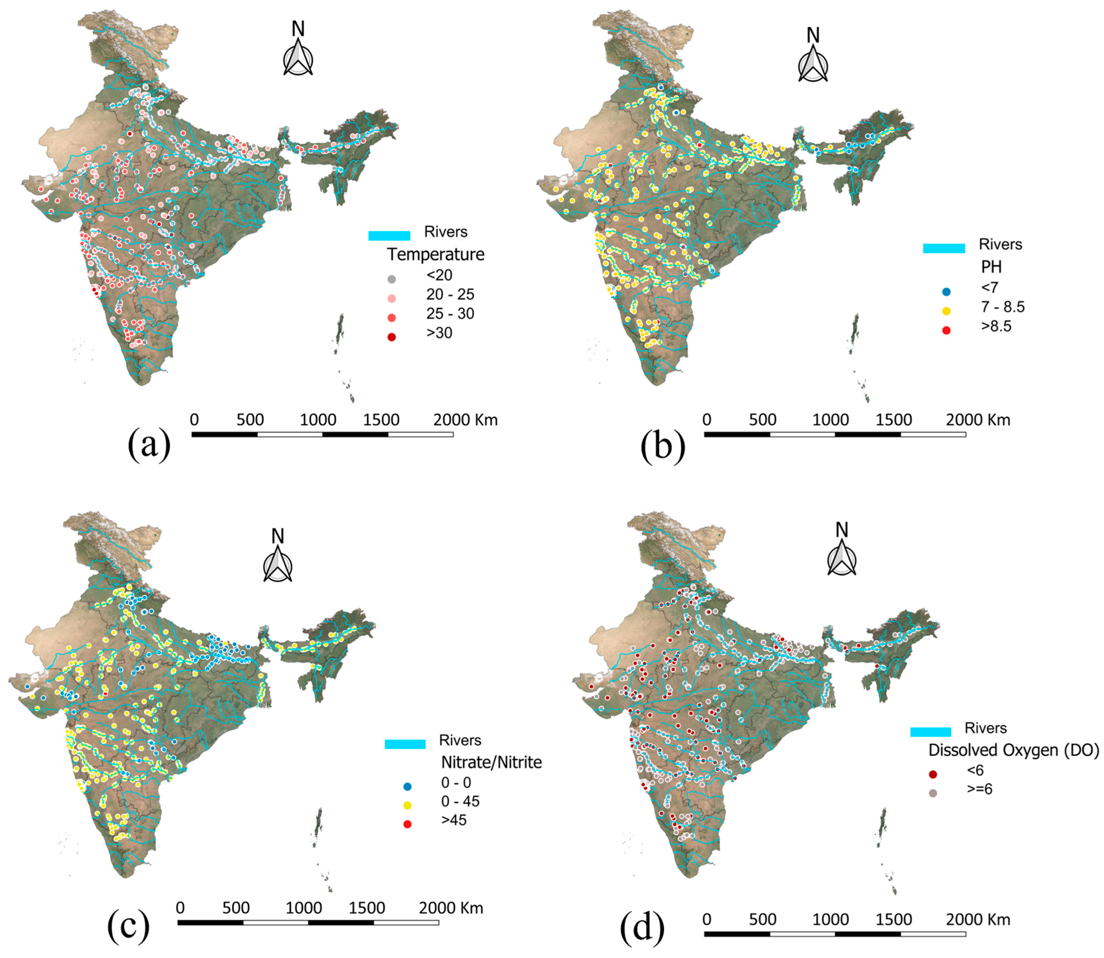
2.11. Geospatial Mapping of Input Features
To visualize the spatial variation in water quality parameters, georeferenced maps were generated for all eight input features using thematic symbology. Each parameter was classified into meaningful environmental categories based on the standard thresholds. The maps display measurement points overlaid on the river networks across India, with color-coded markers representing value ranges for Temperature, pH, DO, BOD, Nitrate/Nitrite concentration, Conductivity, Fecal Coliform, and Total Coliform. These spatial distributions offer an environmental context to the modeling framework and highlight regional trends and anomalies relevant to water quality assessment.
2.12. Software and Computational Environment
All experimental data processing, modeling, statistical analysis, and spatial visualizations were conducted using the following software tools and libraries:
Python version 3.10.11 was used for all programming, model development, and analysis.
Scikit-learn (v1.3.2): For regression and classification modeling, model evaluation, and feature importance analysis. Website:
https://scikit-learn.org/stable/, accessed on 17 July 2025.
Pandas (v2.1.4) and NumPy (v1.26.0): For data handling, transformation, and numerical computations. Websites:
https://pandas.pydata.org/, https://numpy.org/, accessed on 17 July 2025
Matplotlib (v3.8.0) and Seaborn (v0.13.0): For data visualization including correlation heatmaps, residual plots, and classification matrices. Websites:
https://matplotlib.org/, https://seaborn.pydata.org/, accessed on 17 July 2025
Jupyter Notebook (via Anaconda Navigator) was used as the development environment. Website:
https://jupyter.org/, accessed on 17 July 2025
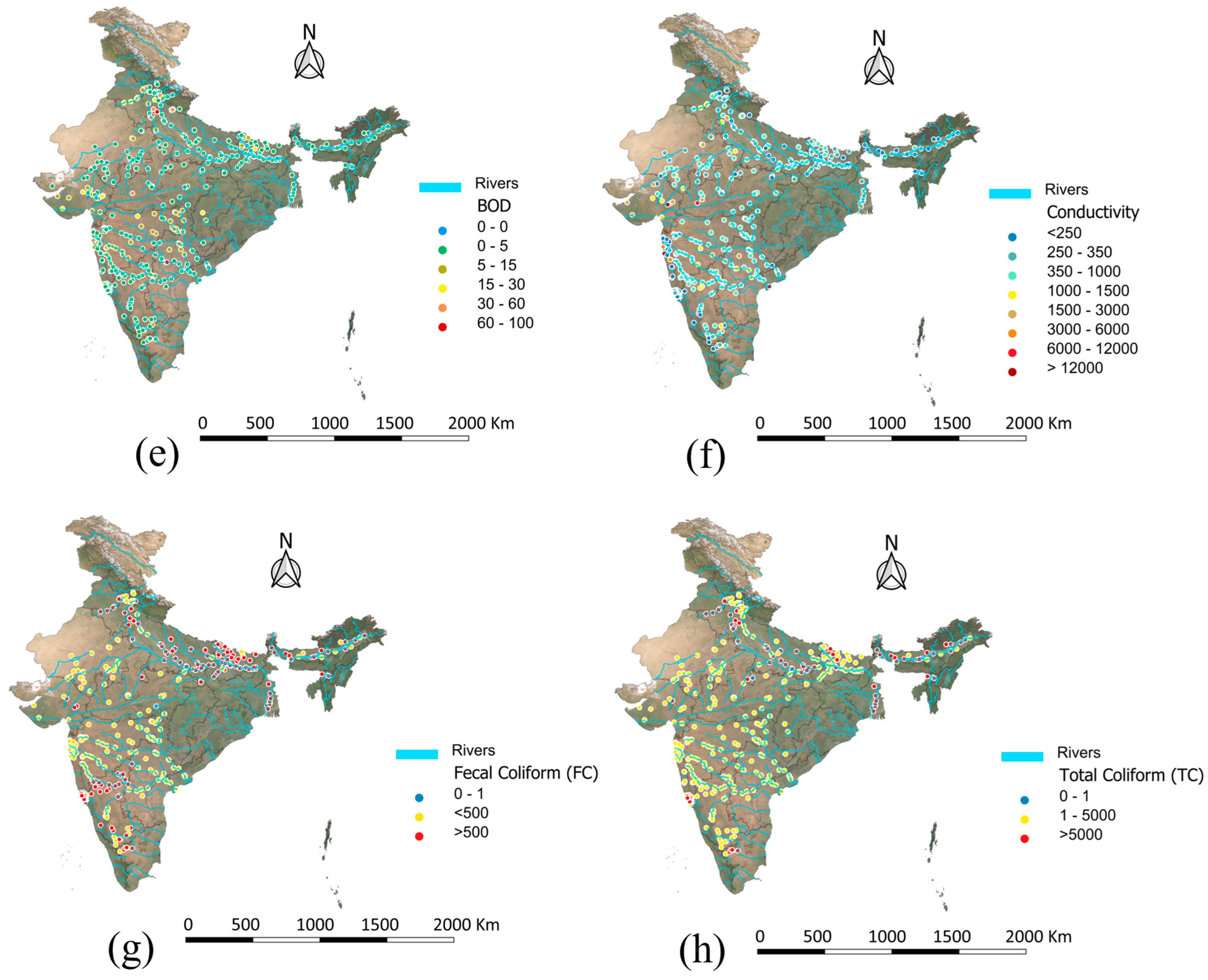
GIS Mapping: Spatial visualizations in Figure 11 (e.g., BOD, Conductivity, Fecal Coliform, and Total Coliform distributions) were generated using tools available in the GIS Lab at the Department of Civil Engineering, Madanapalle Institute of Technology and Science. Spatial data was layered over river basins of India using standard shapefiles and environmental symbology. Software used: QGIS version 3.28. Website:
https://qgis.org/en/site//, accessed on 17 July 2025.
All software and tools were executed on a system running Windows 11 (64-bit) with Intel i7 processor and 16 GB RAM. All scripts and spatial overlays are available from the corresponding author upon request.
3. Results and Discussion
This section presents a comprehensive evaluation of the machine learning framework developed for Water Quality Index (WQI) prediction and classification. It begins with an exploratory data analysis (EDA) to uncover trends, correlations, and feature distributions that shape water quality dynamics. This is followed by quantitative assessments of regression and classification model performance, supported by residual analysis, feature importance interpretation, and misclassification diagnostics. Comparative analysis between ML-driven predictions and manually derived WQI classes further validates the robustness of the proposed models. Finally, spatial visualizations of water quality parameters across India enrich the contextual understanding of regional pollution patterns. Together, these insights build a holistic view of the modeling outcomes and their environmental relevance.
3.1. Exploratory Data Analysis
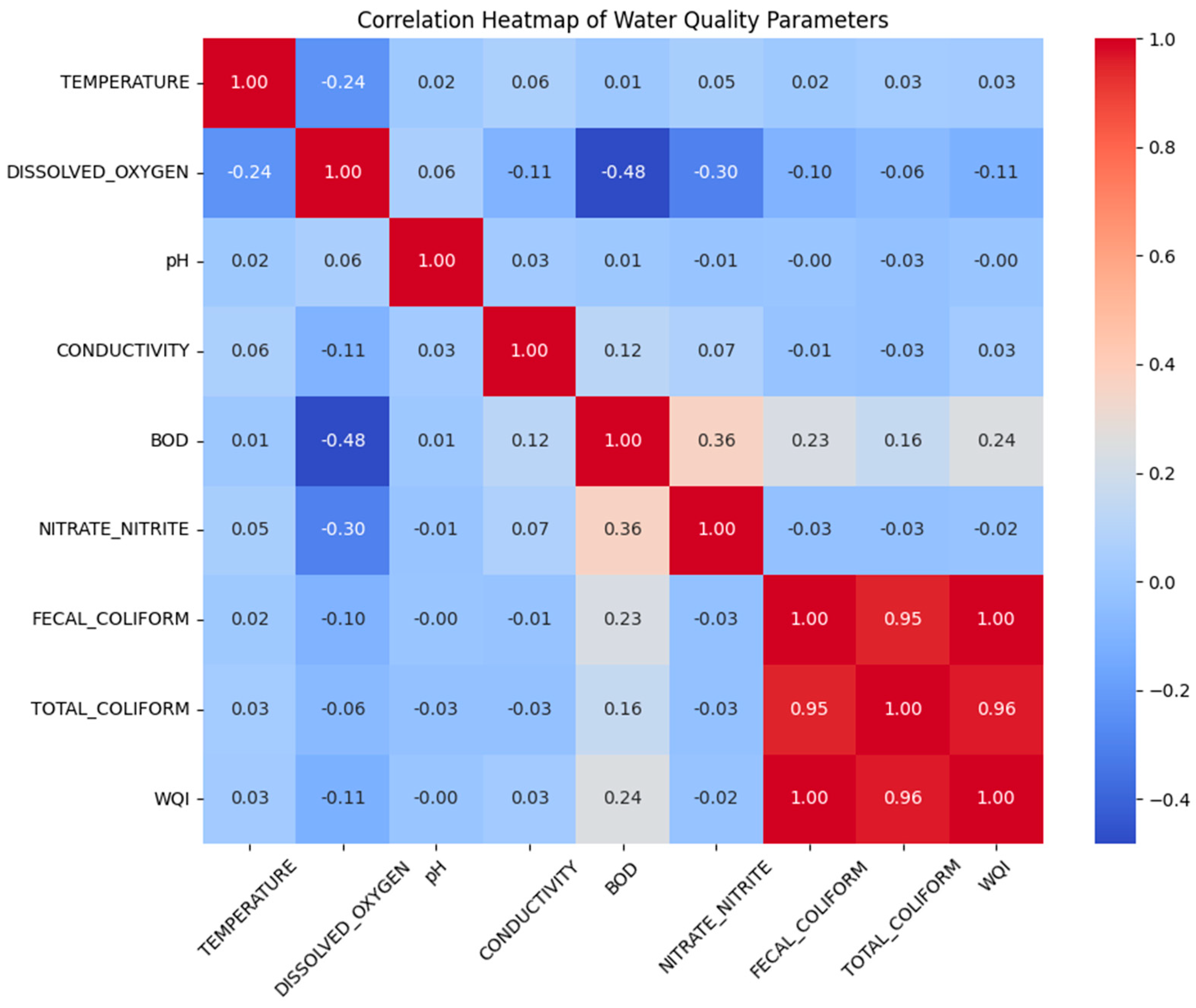
A comprehensive exploratory analysis was conducted to understand the relationships between water quality parameters and their influence on the Water Quality Index (WQI). The correlation heatmap (
Figure 1) revealed strong positive correlations between Fecal Coliform, Total Coliform, and the WQI, while features like Dissolved Oxygen exhibited a weak negative association with BOD and Nitrate/Nitrite, highlighting their ecological interdependence. These correlations served as early indicators of which variables might be more influential in model learning. Although some features exhibit weak linear correlation with the WQI, they were retained in the modeling process to preserve domain completeness and account for possible nonlinear or interaction effects. This approach is further supported by model-based feature importance results in
Section 3.3, where certain weakly correlated variables still contributed meaningfully to prediction accuracy.
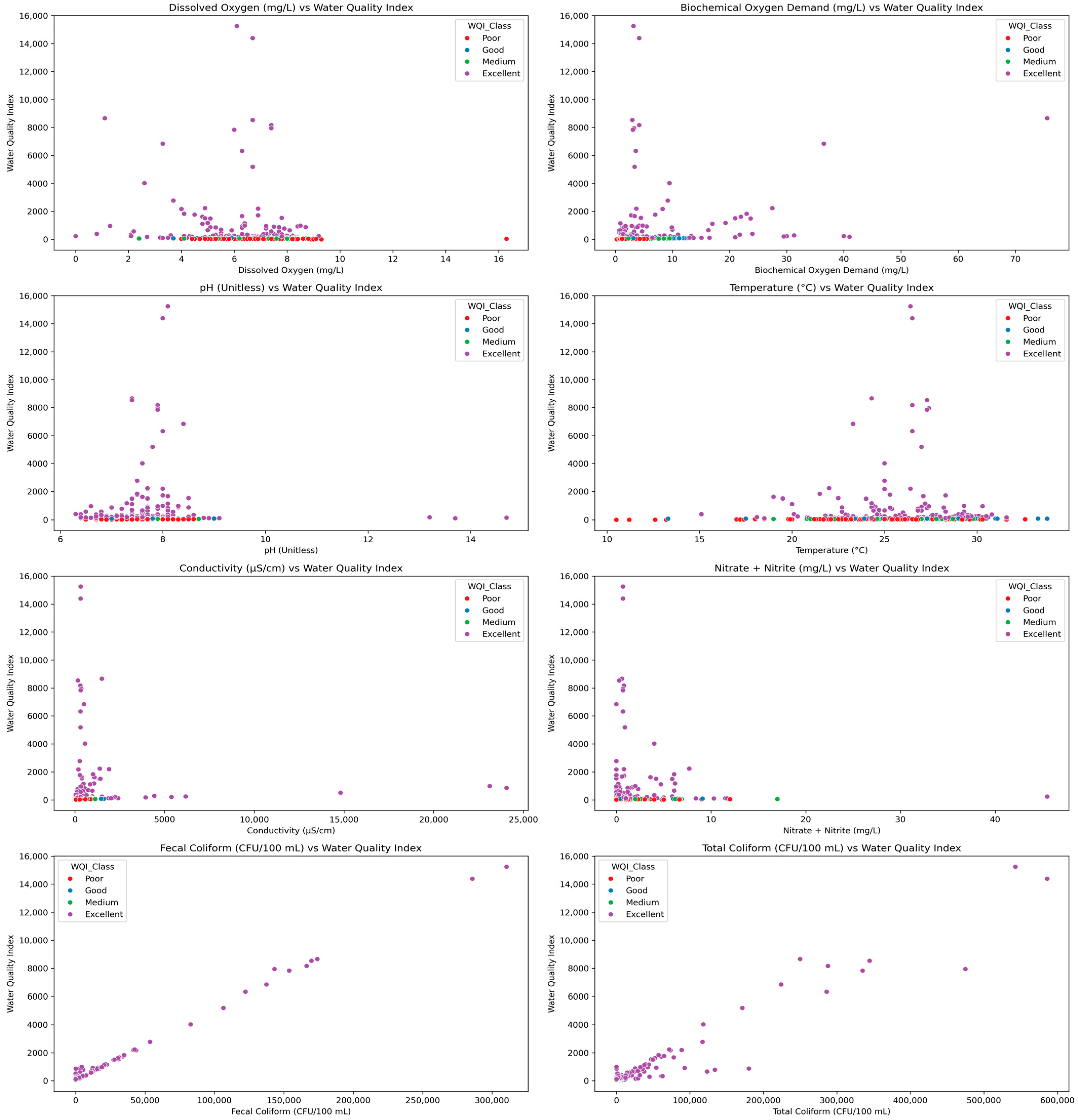
Scatter plots (
Figure 2) comparing individual features with the WQI showed that microbial indicators such as Fecal and Total Coliform had a nonlinear and positively skewed influence, especially in high WQI ranges. Other parameters like pH, Conductivity, and Nitrate/Nitrite displayed less consistent trends, suggesting localized effects or noise.
Violin and strip plots (
Figure 3) stratified by WQI class provided a distributional overview, confirming that poor-quality water samples had substantially higher BOD, microbial counts, and in some cases, higher temperatures. Conversely, Excellent and Good water classes exhibited tighter distributions for these parameters, with lower central tendencies.
Together, these visual diagnostics confirmed distinct patterns across WQI categories and supported the hypothesis that a select group of physicochemical and microbial features disproportionately contributed to water quality assessment. This informed model selection and justified retaining all eight features in the machine learning pipeline.
The trends and interdependencies identified through EDA provided a preliminary understanding of the relative impact of each parameter on WQI outcomes. These visual patterns, particularly the strong associations of microbial indicators and BOD with poor water quality, guided the inclusion of all eight input features in the subsequent modeling pipeline. Further quantification of these influences using model-based feature importance metrics is presented in
Section 3.3, reinforcing and validating the initial observations from this exploratory stage.
3.2. Overview of Modeling Performance
The performance of both regression and classification models was evaluated across training, testing, and validation sets to assess predictive accuracy and generalization capability. For WQI predictions as a continuous variable (
Table 1), Linear Regression demonstrated near-perfect
scores across all the splits, but with relatively high MAE and RMSE on the test set, indicating sensitivity to extreme values despite tight linear fit. Ensemble models show more balanced error profiles: Random Forest yielded moderate MAE and RMSE value with a strong
of 0.9586 on the test set, while Gradient Boosting provided the best compromise between precision and generalization, with an
of 0.9247 and a test RMSE of 192.6. Scatter plots (
Figure 4) of actual vs. predicted WQI for all three regressors confirmed tighter clustering along the identity line for ensemble models, particularly for lower WQI ranges, with Linear Regression showing visible overfitting tendencies.
It is worth noting that the WQI was computed using a Weighted Arithmetic Index method (
Section 2.3), which itself is a linear combination of sub-index values weighted by parameter-specific coefficients. As such, the Linear Regression model effectively mirrors this underlying computation logic, leading to near-perfect
values across all dataset splits. This result validates the deterministic nature of the WQI formula but also highlights the limited capacity of linear models to capture any nonlinearity or complex interactions beyond the predefined weight structure. The red dotted line represents the ideal case where predicted WQI values exactly match the actual values (i.e., y = x). Each blue dot represents a test data point, showing the actual versus predicted WQI for a given model.
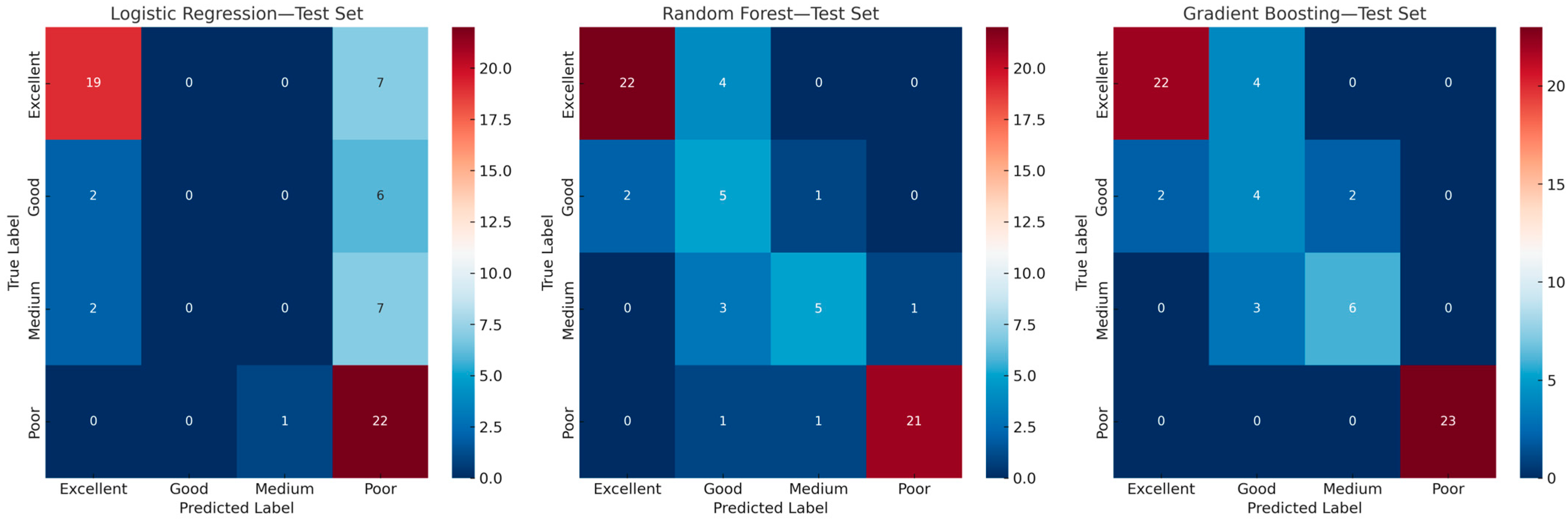
For WQI classification (
Table 2), Logistic Regression underperformed across all the metrics with a test accuracy of 0.61 and a weighted F1-score of 0.54, indicating weak class separation. In contrast, Random Forest and Gradient Boosting models achieved test accuracies of 0.80 and 0.83, respectively, along with F1-scores exceeding 0.81. Confusion matrices (
Figure 5) revealed that Gradient Boosting achieved better differentiation across all classes, especially in correctly predicting the “Poor” and “Excellent” categories with minimal classification. Random Forest also performed well but showed occasional confusion between “Medium” and “Good” classes. Overall, ensemble models outperformed linear models in both regression and classification tasks, offering greater robustness and higher fidelity in modeling the nonlinearities inherent in the WQI system.
3.3. Interpretation of Feature Importance
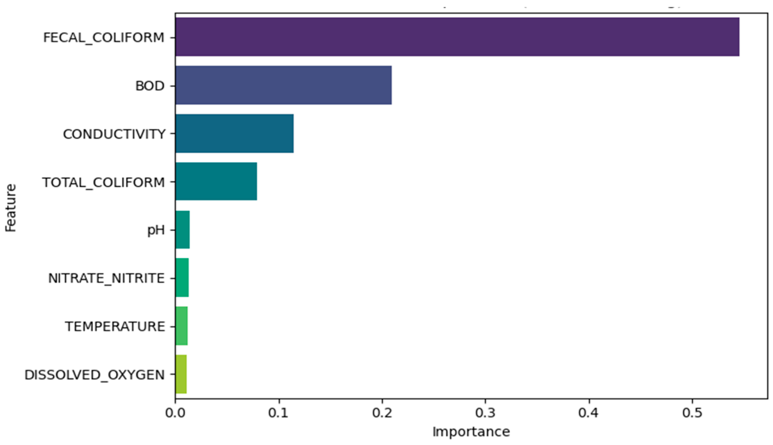
The contribution of individual input variables toward WQI classification was evaluated using both Gini importance (
Figure 6) and Permutation importance (
Figure 7) with Gradient Boosting Classifier serving as the reference model. In both approaches, Fecal Coliform emerged as the most influential feature, indicating its dominant role in determining water quality class. Gini-based analysis placed BOD and Conductivity as the second and third most important features, respectively, followed by Total Coliform. In contrast, permutation importance emphasized the role of Total Coliform over BOD, while still aligning with the broader hierarchy identified through the model’s internal structure.
Parameters like pH, Nitrate/Nitrite concentration, Temperature, and Dissolved Oxygen exhibited lower contributions across both methods, reflecting a limited variance of weaker class separation capacity in the given dataset. These findings reinforce the relevance of microbial and organic load indicators in WQI classification consistent with known environmental standards and health-based thresholds. The agreement across both importance frameworks strengthens the interpretability and credibility of the ML-based predictions.
3.4. Residual and Error Behavior
Residual analysis was conducted using the Gradient Boosting Regressor, the best-performing regression model, to evaluate the error distribution and identify potential biases in WQI predictions. The residual plot (
Figure 8), which charts the difference between actual and predicted WQI values against predicted scores, reveals that most predictions cluster tightly around the zero-error line (denoted by the red dashed line, where perfect predictions would lie), suggesting accurate estimates across a wide range of values. However, a few outliers with large negative residuals indicate instances where the model significantly overpredicted WQI, particularly for high predicted values. This asymmetry suggests that while the model performs well overall, it is susceptible to larger errors in the upper WQI spectrum, possibly due to class imbalance or fewer high-quality water samples in the training set. The general spread, however, remains narrow for the majority of cases, reinforcing the model’s robustness within the most common WQI ranges.
3.5. Misclassification Patterns
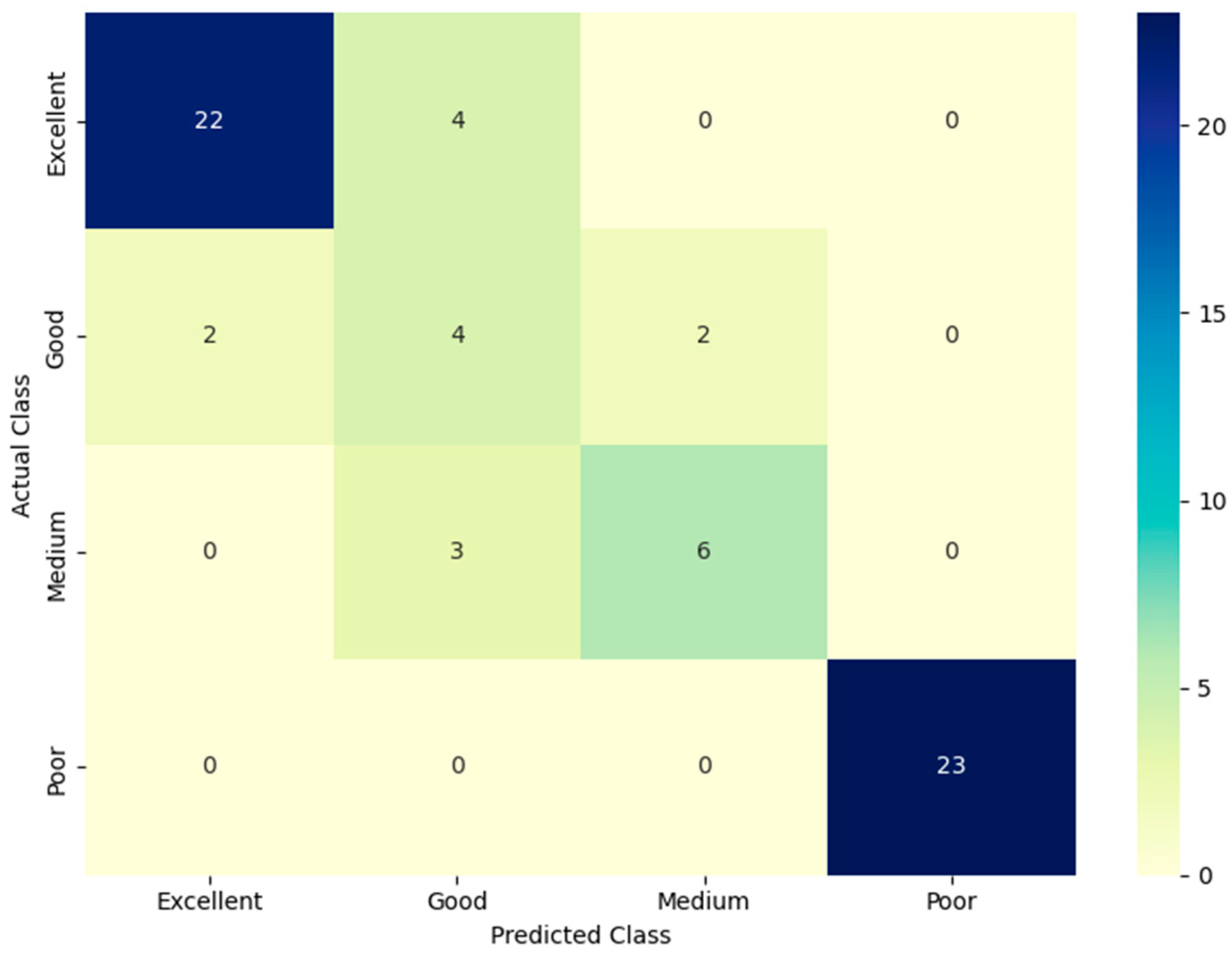
To better understand the behavior of the classification model, misclassification analysis was conducted using predictions from the Gradient Boosting Classifier. The confusion matrix (
Figure 9) highlights strong performance for the “Poor” and “Excellent” classes, with all 23 “Poor” samples and 22 of 26 “Excellent” ones correctly classified. However, confusion between neighboring classes is evident, particularly in the “Good” and “Medium” ranges, where overlapping water quality parameters likely contributed to class boundary ambiguity.
An inspection of the misclassified records (
Table 3) reveals patterns that may explain the classification drift. Several samples labeled “Excellent” were predicted as “Good” despite relatively high coliform levels or marginal DO values, suggesting that nonlinear interactions among features may have pushed them across the decision threshold. Similarly, “Medium” class samples misclassified as “Good” often presented borderline BOD or Conductivity values, indicating close proximity to threshold boundaries in the feature space.
These results imply that the model is highly responsive to minor variations in feature combinations, especially near class boundaries, and such transitions merit further exploration in future rule refinements or ensemble smoothing strategies.
3.6. ML vs. Manual Classification Agreement
To assess the alignment between rule-based WQI classification and ML-driven predictions, a full-sample comparison was conducted on the unseen test set (given in the
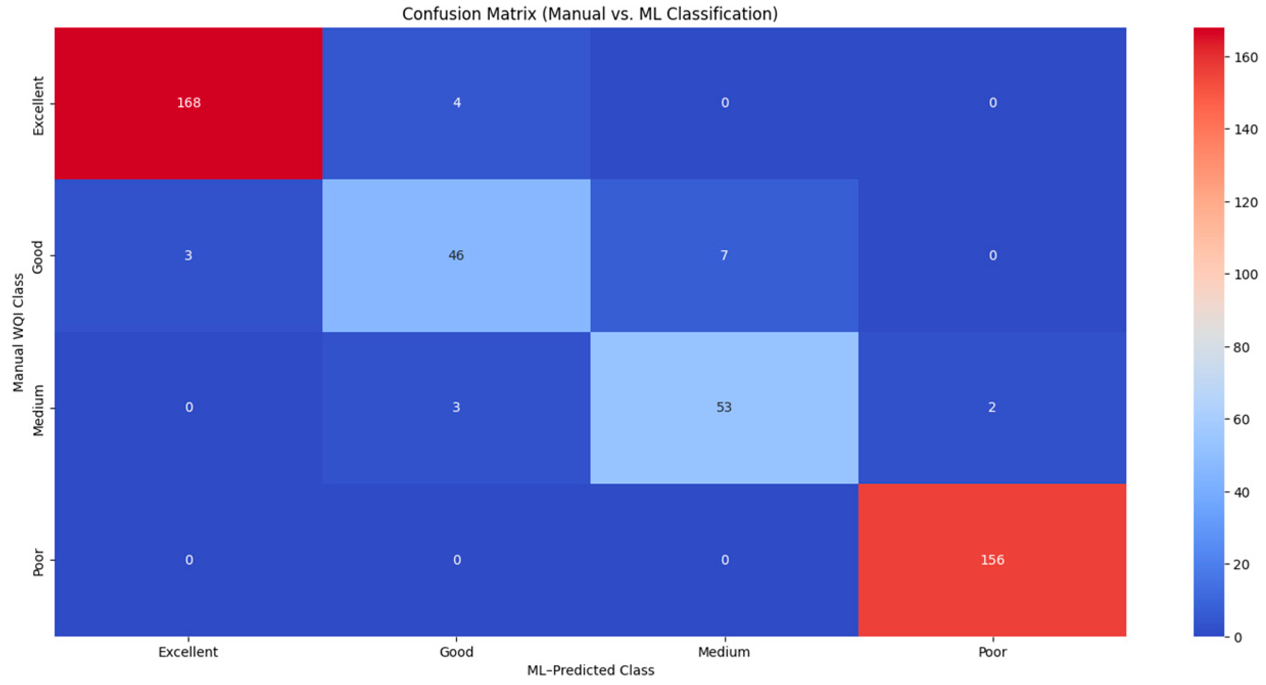
Supplementary File), using manually labeled classes as ground truth. These manual classes were derived directly from thresholding continuous WQI values, whereas the predicted labels were generated by the trained Gradient Boosting Classifier.
The confusion matrix (
Figure 10) confirms a high level of agreement across all four WQI categories, with the “Poor” and “Excellent” classes achieving perfect or near-perfect matches. Minor deviations were observed primarily between “Good” and “Medium” labels, where transitions are typically subtle and data distributions overlap. The overall classification agreement reached 95.7%, indicating strong alignment between manual and ML-predicted classes.
These findings indicate that the ML model not only approximates manual labeling with high fidelity but also holds promise in cases where input features are partially missing, noisy, or span class thresholds–scenarios where static rules might fall short. This analysis underscores the classifier’s robustness while validating its ability to replicate expert-defined labeling under standard conditions.
3.7. Spatial–Contextual Insights
Spatial distribution (
Figure 11) of the eight input parameters provided critical context for understanding regional trends in water quality across India. In
Figure 11a–d, parameters such as Temperature, pH, Nitrate/Nitrite Concentration, and Dissolved Oxygen displayed noticeable geographical clustering. For instance, high-temperature zones were concentrated in southern and central India, while suboptimal pH levels were more prevalent in parts of the exceeding permissible limits and were primarily concentrated in central belt zones, suggesting localized agricultural runoff or contamination sources.
Figure 11e–h showed widespread exceedances across densely populated river basins for the microbial indicators, like Fecal Coliform and Total Coliform, especially in the northern and eastern regions. Similarly, elevated BOD and Conductivity levels were observed in the Indo–Gangetic plains and western India, indicating industrial or domestic pollution hotspots.
These spatial patterns aligned with the variable influence observed in model-based feature importance analyses and highlight the heterogeneity in pollution sources. For instance, features like BOD, Conductivity, and microbial indicators, identified by the model as highly influential, also showed strong regional clustering in known pollution hotspots, supporting their predictive power. The geospatial visualization supports the model’s learned relationships and reinforces the utility of incorporating environmental geography into data-driven water quality management.


 ,
, 


