
Modelling a Lab-Scale Continuous Flow Aerobic Granular Sludge Reactor: Optimisation Pathways for Scale-Up


Abstract
1. Introduction
2. Literature Review
2.1. Conventional Wastewater Treatment Technologies
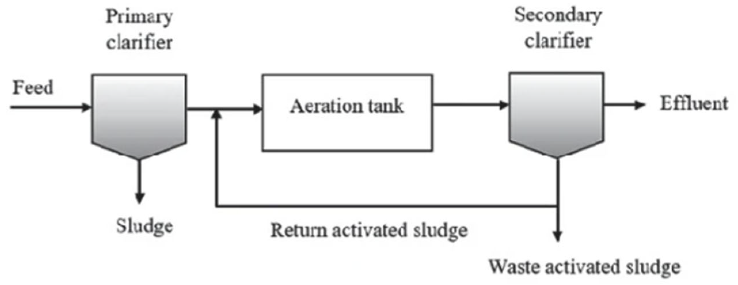
2.1.1. Key Stages of Wastewater Treatment
2.1.2. Comparison of Secondary Treatments
- Low operation and management cost compared to activated sludge.
- Lower sludge generation.
- Large land usage compared to the activated sludge process.
- Lower quality effluent.
- High energy input for aeration.
- Simplicity and reliability.
- Low power requirements.
- The effluent needs additional treatment.
- Odour emission.
- The need for regular operator monitoring.
- Very high-quality effluent.
- Small reactor size.
- Membrane fouling and membrane maintenance.
- Higher power consumption, sometimes double the consumption of activated sludge.
- Higher capital and operational costs.
- Foaming.
- Short retention time.
- Low energy consumption compared to active sludge.
- Low operating cost.
- The need for sludge removal.
- Sensitivity to wastewater characteristics.
2.2. Aerobic Granular Sludge
2.2.1. Composition and Properties of AGS
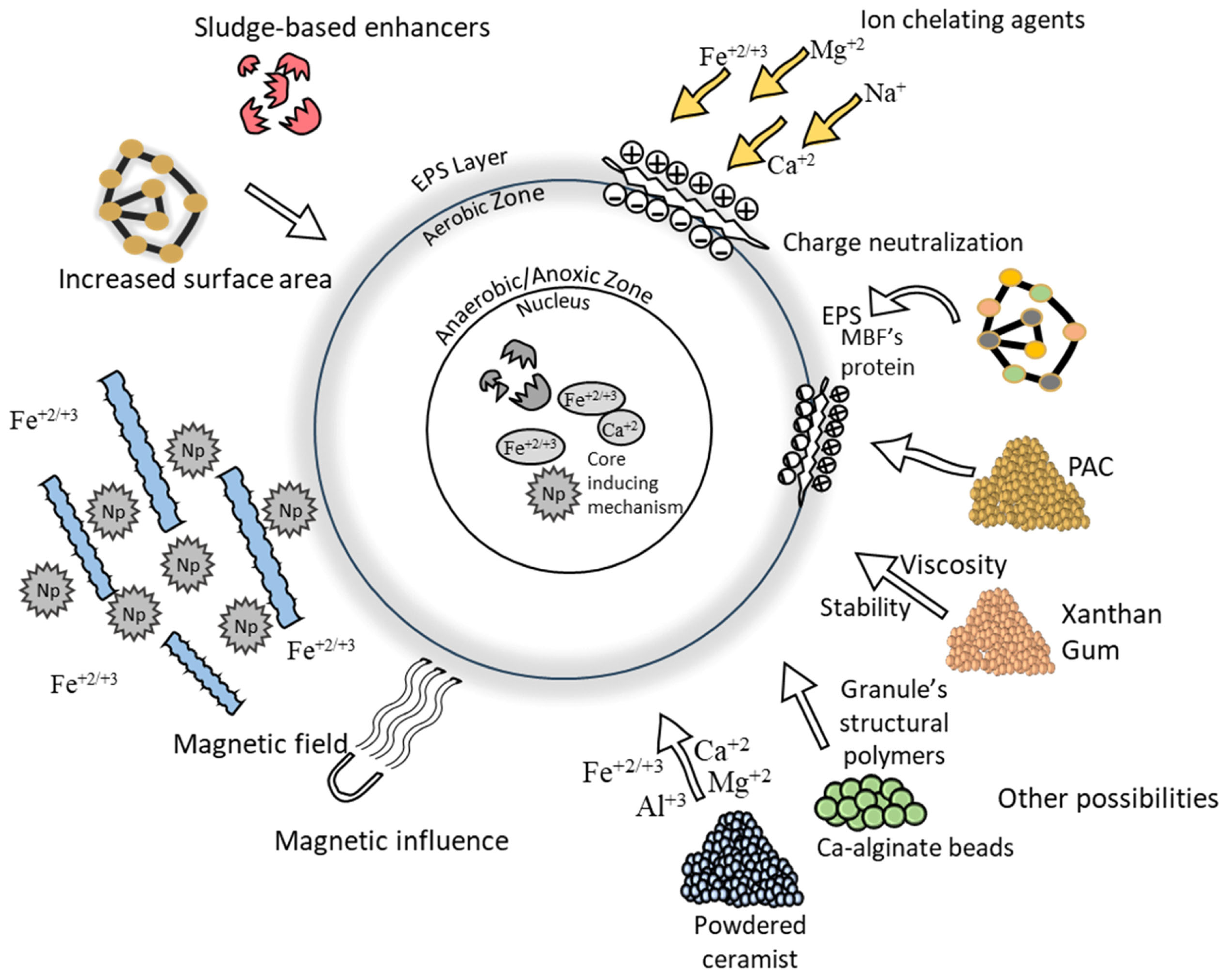
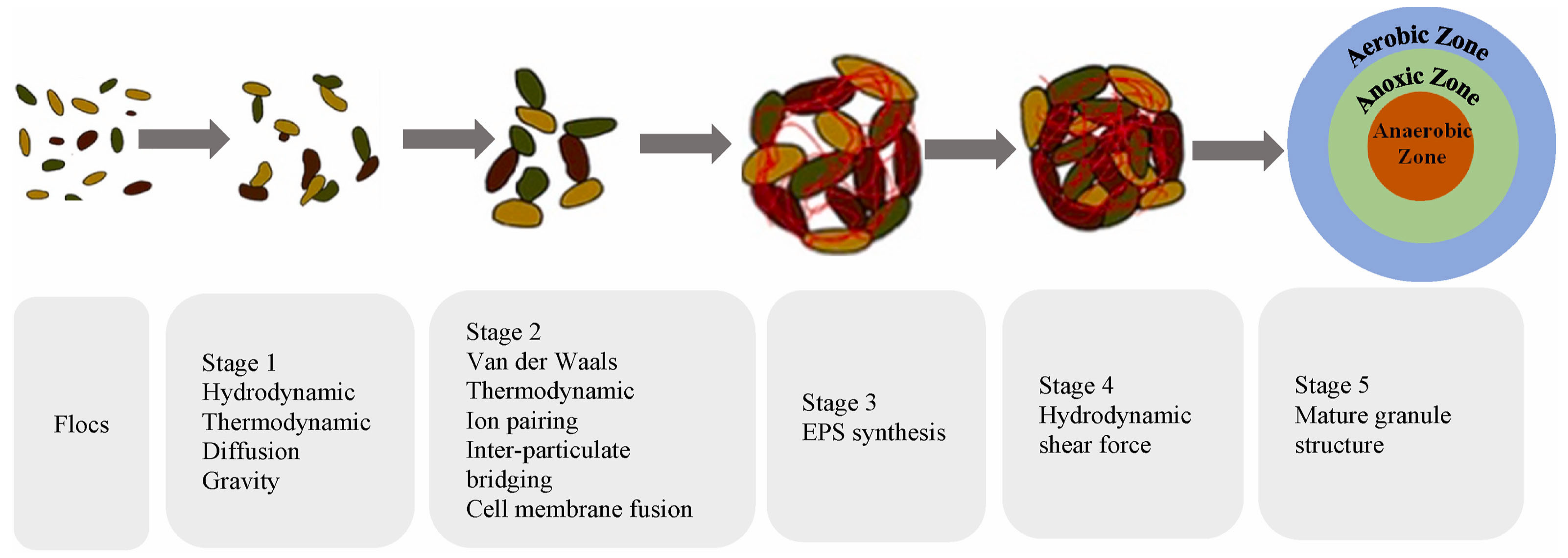
2.2.2. Formation Mechanisms of AGS
The Four-Step Hypothesis
Factors Affecting AGS Formation
2.2.3. AGS in Wastewater Treatment
2.3. Continuous Flow Reactors
2.3.1. Continuous Flow Reactors in Wastewater Treatment
2.3.2. Comparison Between Continuous Flow Reactors and SBRs
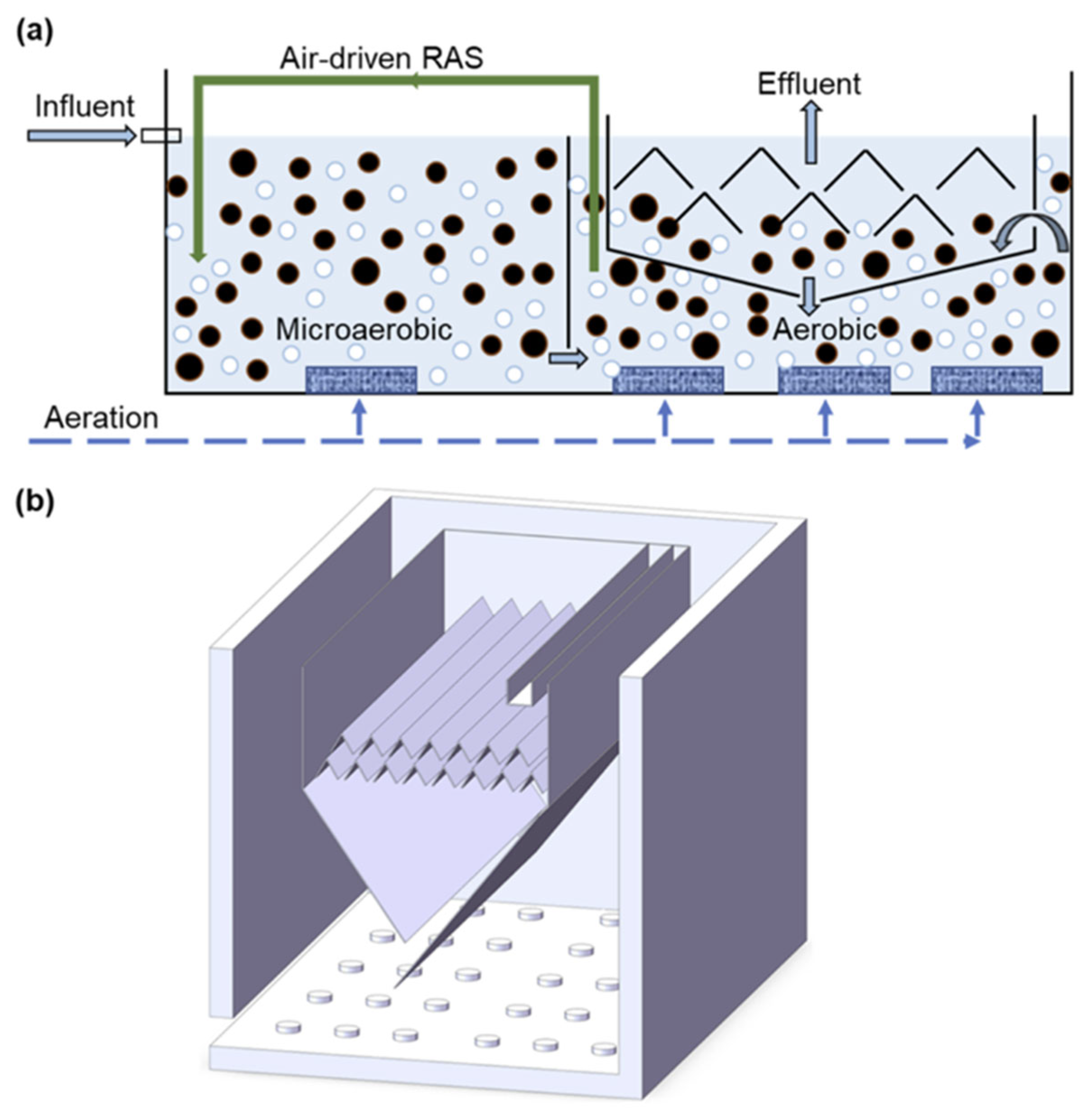
2.3.3. Aerobic Granular Sludge Continuous Flow Reactors
2.4. Knowledge Gaps in AGS Treatment and Future Directions
3. Methods
3.1. Reactor Model
- Steady-state operation due to continuous flow configuration.
- AGS granule shapes are assumed to be perfectly spherical.
- Microbial growth follows a defined Monod kinetic model.
- Monod kinetics assumes reactions are irreversible and only one substrate is limiting [33].
- Due to aerating during the oxic phase, dissolved oxygen is non-limiting.
3.1.1. Microbial Kinetics
3.1.2. Chemical Oxygen Demand (COD)
3.1.3. Mass Transfer
3.1.4. Aeration and Gas Transfer Variables
3.1.5. Heat Transfer
3.1.6. Hydrodynamics and Mixing
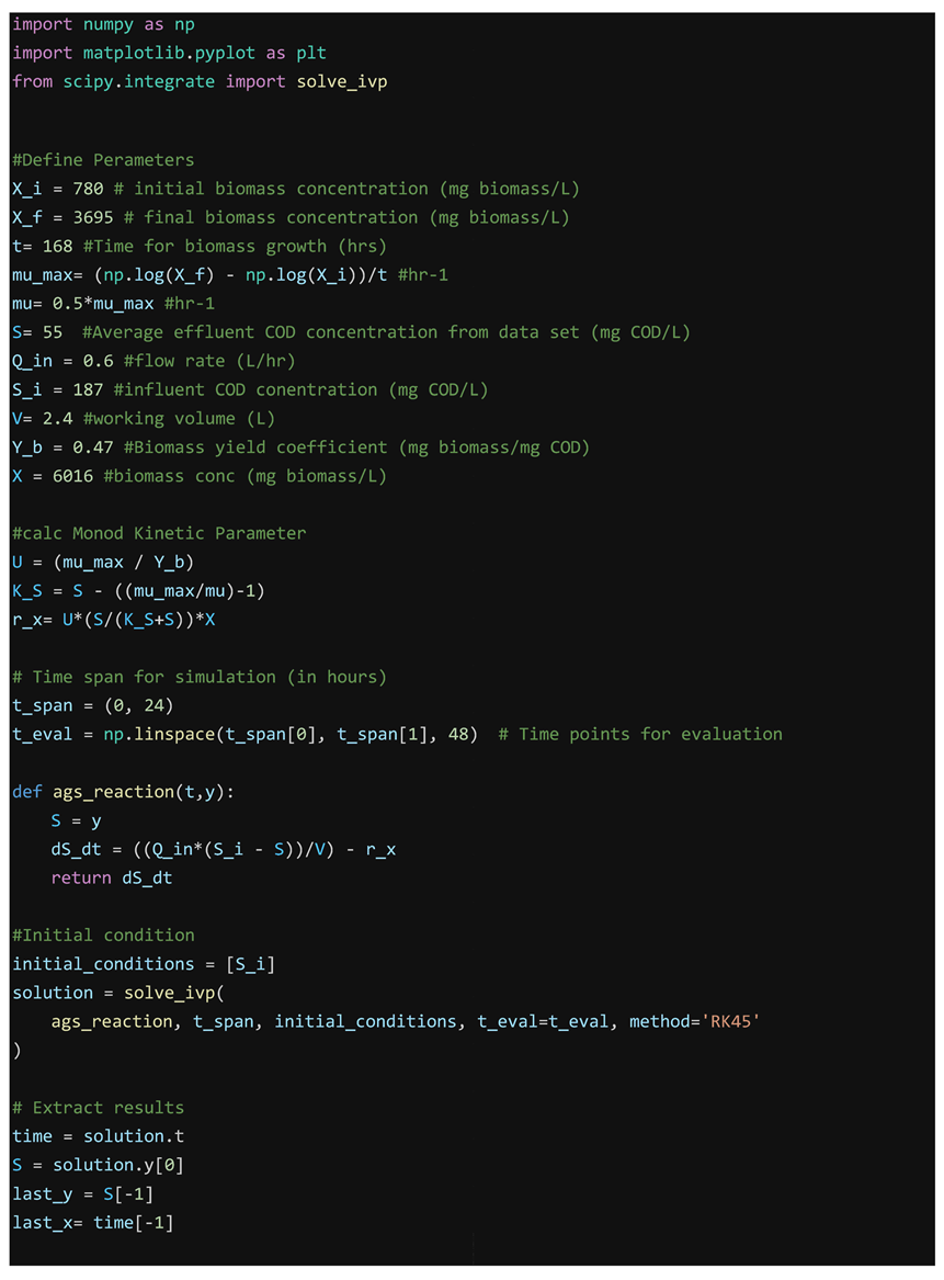
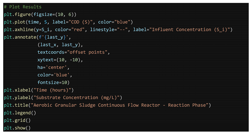
3.2. Python Code
3.3. CFD Model
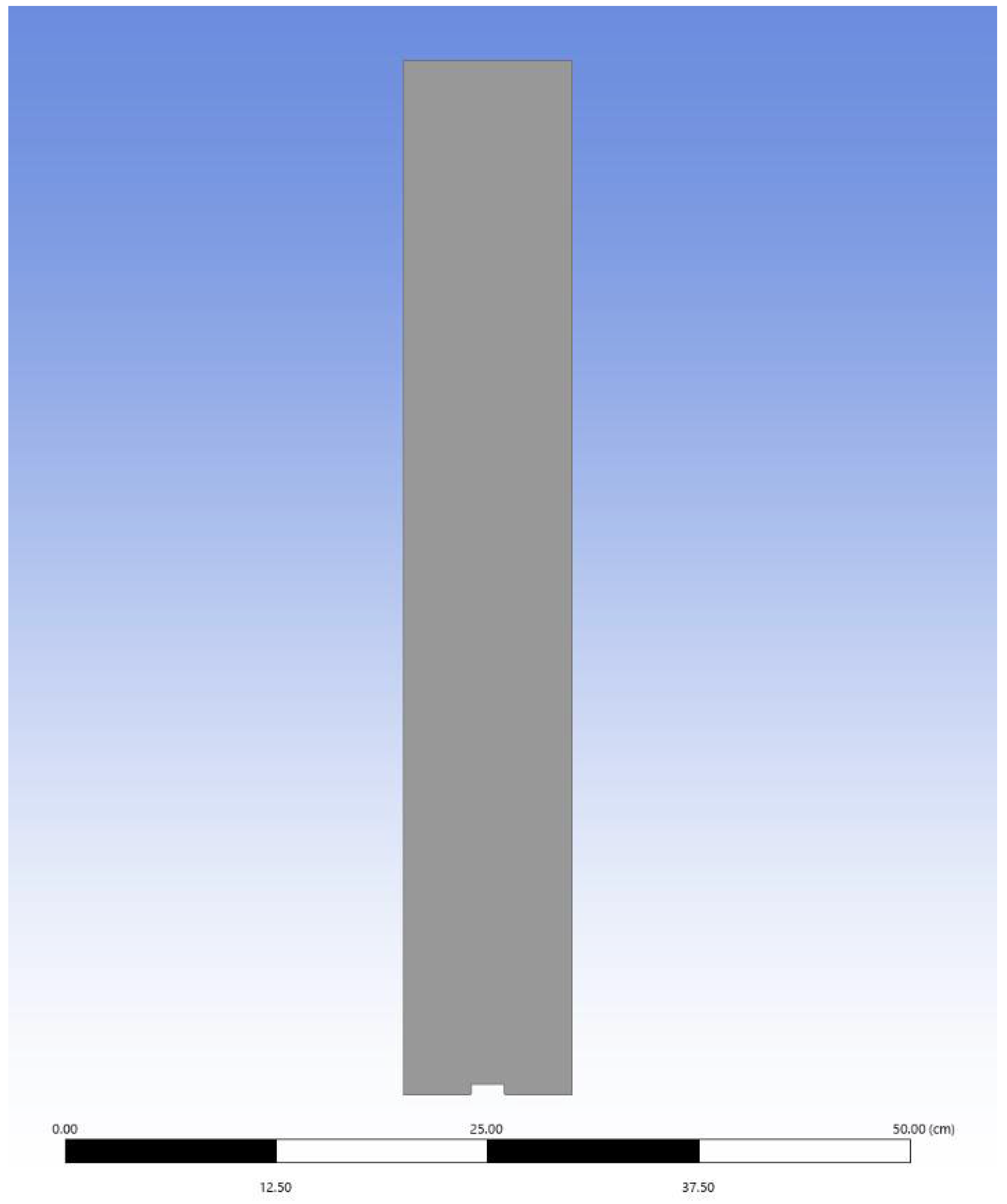
3.3.1. Geometry
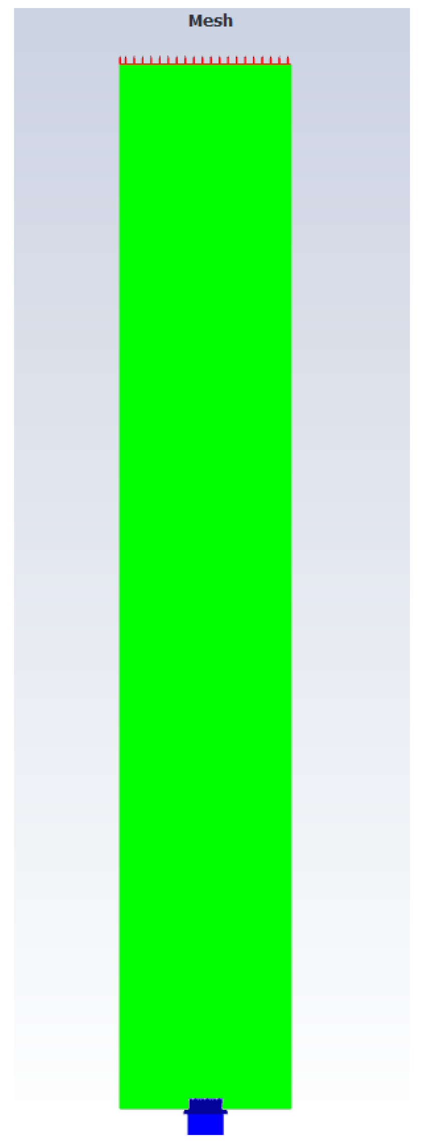
3.3.2. Meshing
3.3.3. Set-Up and Governing Equations
- 1.
- Continuity Equation
- 2.
- Momentum Balance
- 3.
- Energy Balance
- 4.
- Wall shear stress
Non-Equilibrium Wall Function
4. Results and Discussion
4.1. Mathematical Reactor Model
4.1.1. Microbial Kinetics

| Parameter | Symbol | Calculated Value | Referenced Values | Citation |
|---|---|---|---|---|
| Maximum specific growth rate | μmax | 0.22 d−1 = 0.0092 h−1 | 0.266 h−1 | |
| Half-saturation constant | Ks | 55 mg L−1 | ||
| Biomass Yield Coefficient | YB | 0.47 mg biomass/mg COD | 0.24–0.68 mg biomass/mg COD 0.33–0.37 mg biomass/mg COD | [38] [39] |
| Decay coefficient | b | 0.0059 h−1 |
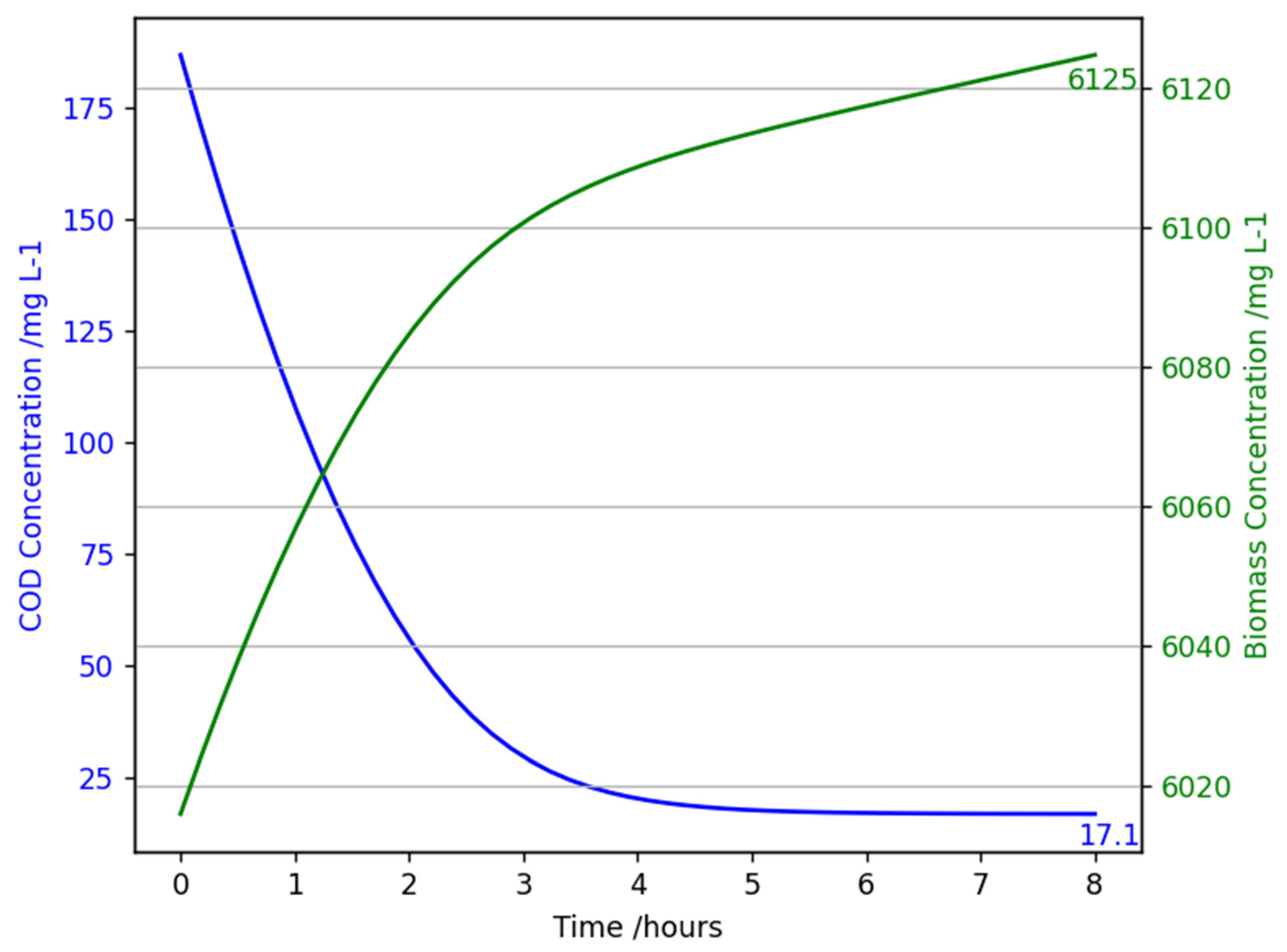
4.1.2. Chemical Oxygen Demand (COD)
| Parameter | Symbol | Calculated Value | Referenced Values | Citation |
|---|---|---|---|---|
| Flow rate | Qi | 0.6 L h−1 | ||
| Specific substrate utilisation rate | Umax | 0.022 mg COD mg biomass-1 h−1 | ||
| COD degradation rate constant | rx | 59.8 h−1 | ||
| Effluent total COD concentration | Se | 32 mg L−1 | ||
| COD removal efficiency (%) | 82.8% | ~80% | [42] | |
| ~96 ± 2.7% | [21] | |||
| 97% | [31] |
4.1.3. Mass Transfer
- Moles of O2, NO2 = 0.008725 mol L−1
- Oxygen concentration in the gas phase = 280 mg L−1
4.1.4. Aeration and Gas Transfer Variables
- Oxygen transfer rate = oxygen uptake rate = 211 mg O2/L/h
- Aeration flow rate = 0.000184 m3 s−1
4.1.5. Heat Transfer
- Mass flow rate = 14.4 kg h−1
- Heat transfer rate (W) = 0.0202 W
- Overall heat transfer coefficient = 0.084 W/m2 °C
4.1.6. Hydrodynamics and Mixing
4.2. Python Code Sensitivity Analysis
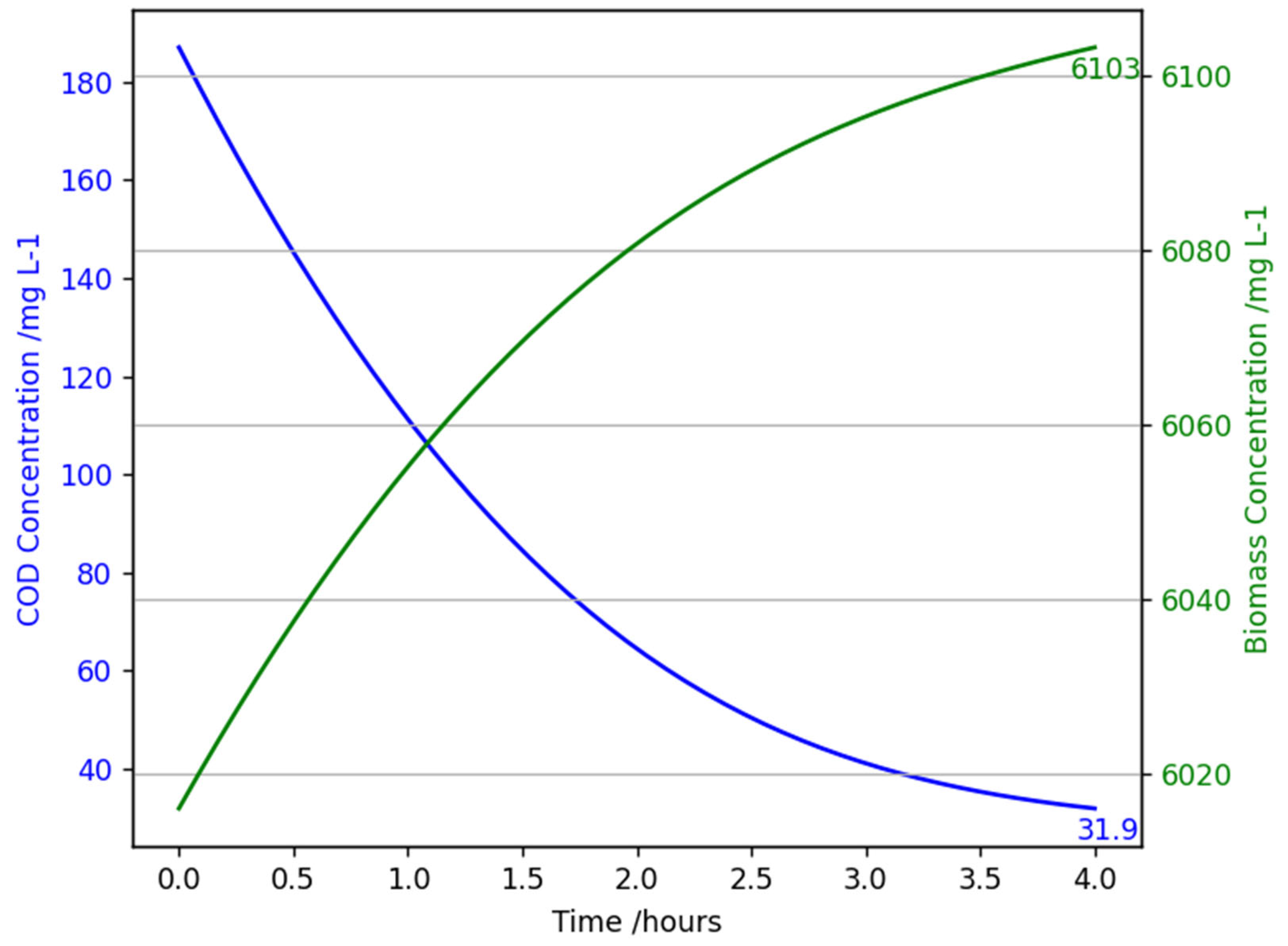
4.2.1. Standard Mathematical Model Python Results
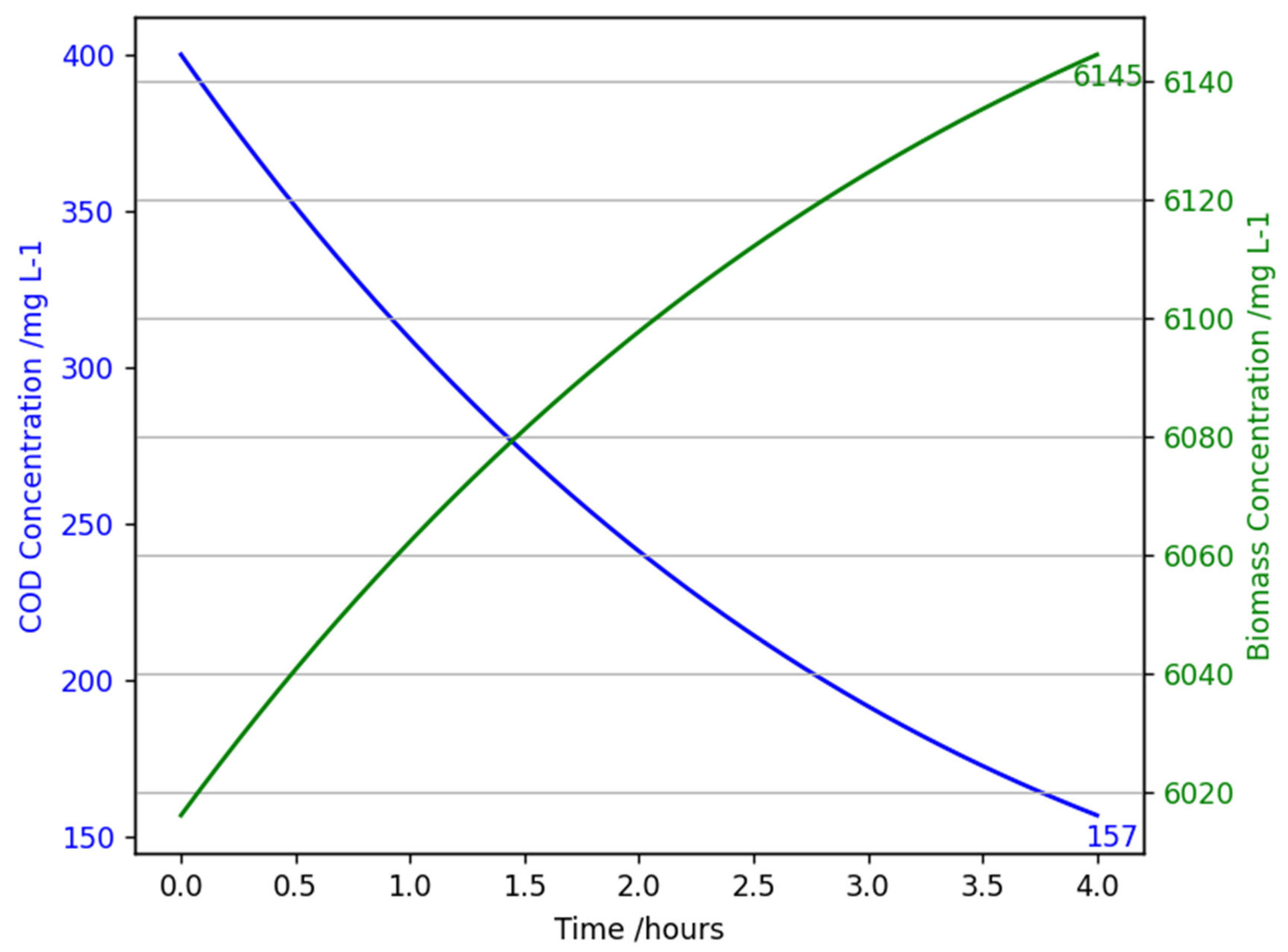
4.2.2. High COD Concentration Sensitivity Analysis Results
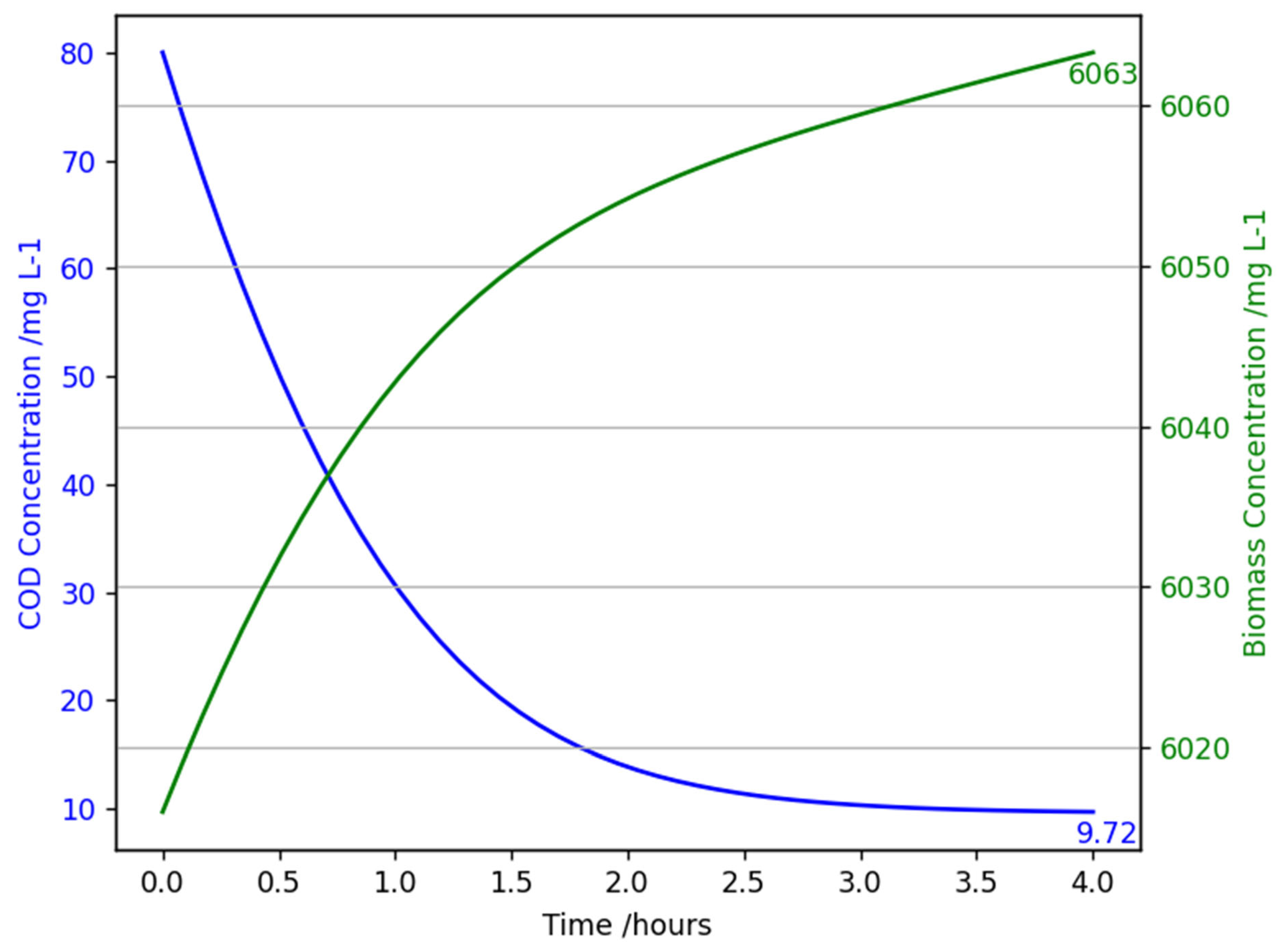
4.2.3. Low COD Concentration Sensitivity Analysis
4.2.4. High Flow Rate Sensitivity Analysis
4.2.5. Low Flow Rate Sensitivity Analysis
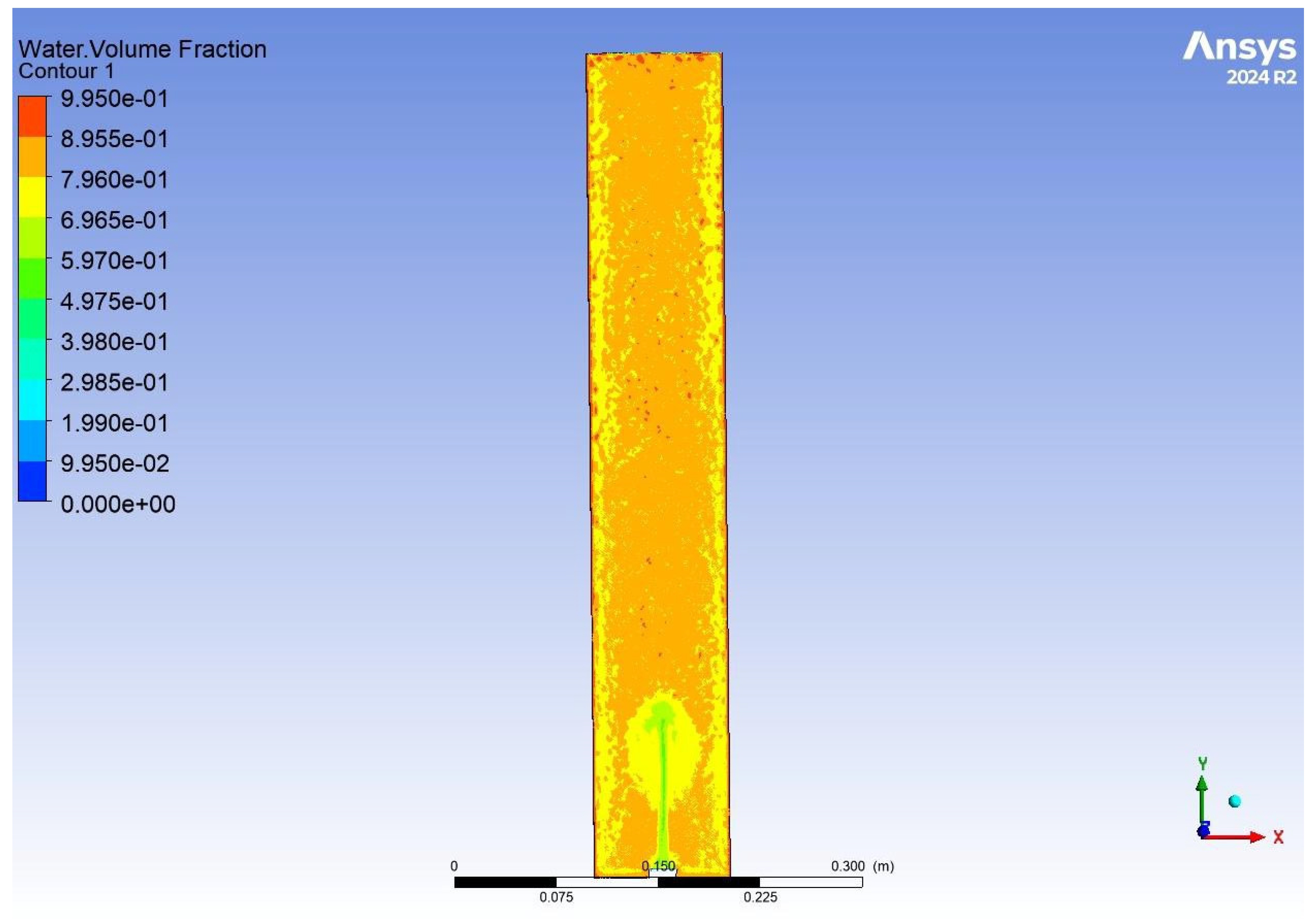
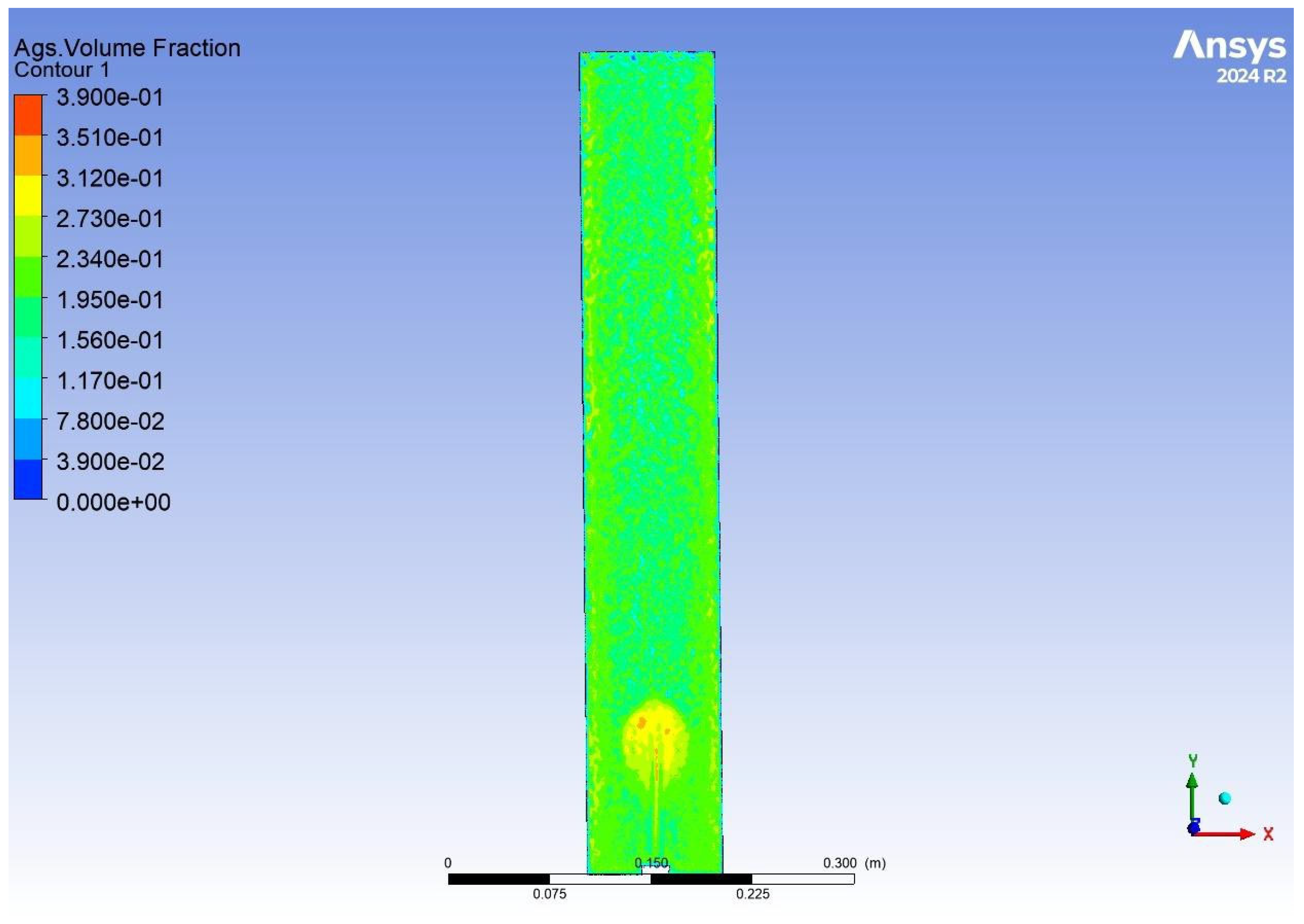
4.3. CFD Results
5. Future Recommendations
- First due to the many limitations of the currently available computational resources, performing a 3D CFD simulation needs to be conducted on a computer unit equipped with ultra-fast processors and efficient cooling systems. This would enable the formation of a refined mesh small enough to pick up the interactions between small air bubbles, granular sludge and water. Improved computational capacity would run calculations quicker, leading to providing more accurate CFD results for the reactor model.
- To investigate reactor configurations which can effectively treat unstable influent conditions, my recommendation is to perform a lab-scale set-up of 2 continuous flow reactors in series with alternating, intermittent aeration. This set-up allows a higher retention time for when high concentration and high flow rate feeds are used, therefore improving reactor performance and stability in real-world scenarios. Also, the reactor design is simple, which is important for considering scale-up as many current continuous flow configurations are too complicated to be applied at large scales. Intermittent aeration will allow small settling periods in continuous operation, reducing the amount of biomass washout. With this set-up, performance evaluations should be conducted regarding varying HRTs and aeration flow rates.
- Finally, more research on pilot-scale reactors is necessary when scaling up from a laboratory to a successful full-scale application. This has not been widely applied in the AGS research field. Therefore, future work should use the same height-to-diameter ratio to develop the mathematical model in this study to guide scale-up efforts. Also using computational fluid dynamics simulations, predictions of reactor performance can be made. Modelling the two reactors in series as stated before should be prioritised, as it will determine if the configuration can achieve the desired performance for real-world influent variations.
6. Conclusions
Author Contributions
Funding
Data Availability Statement
Conflicts of Interest
Appendix A

References
- Yan, J.-L.; Cui, Y.-W.; Huang, J.-L. Continuous flow reactors for cultivating aerobic granular sludge: Configuration innovation, principle and research prospect. J. Chem. Technol. Biotechnol. 2021, 96, 2721–2734. [Google Scholar] [CrossRef]
- Waste Water Treatment Works: Treatment Monitoring and Compliance Limits. Available online: https://www.gov.uk/government/publications/waste-water-treatment-works-treatment-monitoring-and-compliance-limits/waste-water-treatment-works-treatment-monitoring-and-compliance-limits?utm_source=chatgpt.com#lut-for-bod-and-cod (accessed on 19 November 2024).
- Liu, S.; Zhou, M.; Daigger, G.T.; Huang, J.; Song, G. Granule formation mechanism, key influencing factors, and resource recycling in aerobic granular sludge (AGS) wastewater treatment: A review. J. Environ. Manag. 2023, 338, 117771. [Google Scholar] [CrossRef] [PubMed]
- Gandhi, V.; Shah, K. Advances in Wastewater Treatment I; Materials Research Forum LLC: Millersville, PA, USA, 2021. [Google Scholar]
- Kato, S.; Kansha, Y. Comprehensive review of industrial wastewater treatment techniques. Environ. Sci. Pollut. Res. 2024, 31, 51064–51097. [Google Scholar] [CrossRef] [PubMed]
- Kesari, K.K.; Soni, R.; Jamal, Q.M.S.; Tripathi, P.; Lal, J.A.; Jha, N.K.; Siddiqui, M.H.; Kumar, P.; Tripathi, V.; Ruokolainen, J. Wastewater Treatment and Reuse: A Review of its Applications and Health Implications. Water Air Soil Pollut. 2021, 232, 208. [Google Scholar] [CrossRef]
- Jain, R.K.; Cui, Z.C.; Domen, J.K. (Eds.) Chapter 4—Environmental Impacts of Mining. In Environmental Impact of Mining and Mineral Processing; Butterworth-Heinemann: Boston, MA, USA, 2016; pp. 53–157. [Google Scholar] [CrossRef]
- Zagklis, D.P.; Bampos, G. Tertiary Wastewater Treatment Technologies: A Review of Technical, Economic, and Life Cycle Aspects. Processes 2022, 10, 2304. [Google Scholar] [CrossRef]
- Tran, H.T.; Lesage, G.; Lin, C.; Nguyen, T.B.; Bui, X.-T.; Nguyen, M.K.; Nguyen, D.H.; Hoang, H.G.; Nguyen, D.D. Chapter 3—Activated sludge processes and recent advances. In Current Developments in Biotechnology and Bioengineering; Bui, X.-T., Nguyen, D.D., Nguyen, P.-D., Ngo, H.H., Pandey, A., Eds.; Elsevier: Amsterdam, The Netherlands, 2022; pp. 49–79. [Google Scholar] [CrossRef]
- Islam, M.D.; Mahdi, M.M. Chapter 1—Evaluation of micro-pollutants removal from industrial wastewater using conventional and advanced biological treatment processes. In Biodegradation and Detoxification of Micropollutants in Industrial Wastewater; Haq, I., Kalamdhad, A.S., Shah, M.P., Eds.; Elsevier: Amsterdam, The Netherlands, 2022; pp. 1–26. [Google Scholar] [CrossRef]
- Mahlangu, O.T.; Nthunya, L.N.; Motsa, M.M.; Richards, H.; Mamba, B.B. Chapter 12—Treatment of trace organics and emerging contaminants using traditional and advanced technologies. In Development in Wastewater Treatment Research and Processes; Shah, M.P., Ed.; Elsevier: Amsterdam, The Netherlands, 2023; pp. 243–264. [Google Scholar] [CrossRef]
- Yeasmin, F.; Rasheduzzaman, M.; Manik, M.; Hasan, M.M. Activated Sludge Process for Wastewater Treatment. In Advanced and Innovative Approaches of Environmental Biotechnology in Industrial Wastewater Treatment; Shah, M.P., Ed.; Springer Nature: Singapore, 2023; pp. 23–50. [Google Scholar] [CrossRef]
- Luo, B.; He, H.; Yan, Y.; Wang, Y.; Yang, X.; Liu, Y.; Xu, J.; Huang, W. Flocculants for the High-Concentration Activated Sludge Method and the Effectiveness of Urban Wastewater Treatment. Water 2024, 16, 2281. [Google Scholar] [CrossRef]
- Al-Asheh, S.; Bagheri, M.; Aidan, A. Membrane bioreactor for wastewater treatment: A review. Case Stud. Chem. Environ. Eng. 2021, 4, 100109. [Google Scholar] [CrossRef]
- Siatou, A.; Manali, A.; Gikas, P. Energy Consumption and Internal Distribution in Activated Sludge Wastewater Treatment Plants of Greece. Water 2020, 12, 1204. [Google Scholar] [CrossRef]
- Campos, J.L.; Valenzuela-Heredia, D.; Pedrouso, A.; Val del Río, A.; Belmonte, M.; Mosquera-Corral, A. Greenhouse Gases Emissions from Wastewater Treatment Plants: Minimization, Treatment, and Prevention. J. Chem. 2016, 2016, 3796352. [Google Scholar] [CrossRef]
- Ekholm, J.; Persson, F.; de Blois, M.; Modin, O.; Gustavsson, D.J.I.; Pronk, M.; van Loosdrecht, M.C.M.; Wilén, B.-M. Microbiome structure and function in parallel full-scale aerobic granular sludge and activated sludge processes. Appl. Microbiol. Biotechnol. 2024, 108, 334. [Google Scholar] [CrossRef] [PubMed]
- United Kingdom—Kendal, n.d. Nereda a product of Royal HaskoningDHV [Online]. Available online: https://nereda.royalhaskoningdhv.com/en/projects/united-kingdom-kendal (accessed on 19 November 2024).
- Purba, L.D.A.; Ibiyeye, H.T.; Yuzir, A.; Mohamad, S.E.; Iwamoto, K.; Zamyadi, A.; Abdullah, N. Various applications of aerobic granular sludge: A review. Environ. Technol. Innov. 2020, 20, 101045. [Google Scholar] [CrossRef]
- Rosa-Masegosa, A.; Muñoz-Palazon, B.; Gonzalez-Martinez, A.; Fenice, M.; Gorrasi, S.; Gonzalez-Lopez, J. New Advances in Aerobic Granular Sludge Technology Using Continuous Flow Reactors: Engineering and Microbiological Aspects. Water 2021, 13, 1792. [Google Scholar] [CrossRef]
- Hamza, R.A.; Iorhemen, O.T.; Zaghloul, M.S.; Tay, J.H. Rapid formation and characterization of aerobic granules in pilot-scale sequential batch reactor for high-strength organic wastewater treatment. J. Water Process Eng. 2018, 22, 27–33. [Google Scholar] [CrossRef]
- Dawen, G.; Nabi, M. Aerobic Granular Sludge. In Novel Approaches Towards Wastewater Treatment: Effective Strategies and Techniques; Dawen, G., Nabi, M., Eds.; Springer Nature: Cham, Switzerland, 2024; pp. 91–165. [Google Scholar] [CrossRef]
- Kan, X.; Ji, B.; Zhang, J.; Liu, Z.; Xu, Y.; Zhao, L.; Shi, B.; Pu, J.; Zhang, Z. Advances in aerobic granular sludge stabilization in wastewater. Desalination Water Treat. 2024, 319, 100513. [Google Scholar] [CrossRef]
- Hamza, R.; Rabii, A.; Ezzahraoui, F.; Morgan, G.; Iorhemen, O.T. A review of the state of development of aerobic granular sludge technology over the last 20 years: Full-scale applications and resource recovery. Case Stud. Chem. Environ. Eng. 2022, 5, 100173. [Google Scholar] [CrossRef]
- Nancharaiah, Y.V.; Sarvajith, M. Aerobic granular sludge process: A fast growing biological treatment for sustainable wastewater treatment. Curr. Opin. Environ. Sci. Health 2019, 12, 57–65. [Google Scholar] [CrossRef]
- Praveenkumar, T.R.; Alahmadi, T.A.; Salmen, S.H.; Verma, T.N.; Gupta, K.K.; Gavurová, B.; Sekar, M. Impact of sludge density and viscosity on continuous stirred tank reactor performance in wastewater treatment by numerical modelling. J. Taiwan Inst. Chem. Eng. 2024, 166, 105368. [Google Scholar] [CrossRef]
- Fadillah, G.; Alarifi, N.T.S.; Suryawan, I.W.K.; Saleh, T.A. Advances in designed reactors for water treatment process: A review highlighting the designs and performance. J. Water Process Eng. 2024, 63, 105417. [Google Scholar] [CrossRef]
- Samaei, S.H.-A.; Chen, J.; Xue, J. Current progress of continuous-flow aerobic granular sludge: A critical review. Sci. Total Environ. 2023, 875, 162633. [Google Scholar] [CrossRef] [PubMed]
- Haaksman, V.A.; van Dijk, E.J.H.; Al-Zuhairy, S.; Mulders, M.; Loosdrecht MCMvan Pronk, M. Utilizing anaerobic substrate distribution for growth of aerobic granular sludge in continuous-flow reactors. Water Res. 2024, 257, 121531. [Google Scholar] [CrossRef] [PubMed]
- Yu, C.; Wang, K.; Zhang, K.; Liu, R.; Zheng, P. Full-scale upgrade activated sludge to continuous-flow aerobic granular sludge: Implementing microaerobic-aerobic configuration with internal separators. Water Res. 2024, 248, 120870. [Google Scholar] [CrossRef] [PubMed]
- Long, B.; Yang, C.; Pu, W.; Yang, J.; Liu, F.; Zhang, L.; Cheng, K. Rapid cultivation of aerobic granular sludge in a continuous flow reactor. J. Environ. Chem. Eng. 2015, 3 Pt A, 2966–2973. [Google Scholar] [CrossRef]
- Hodaifa, G.; Paladino, O.; Malvis, A.; Seyedsalehi, M.; Neviani, M. Chapter 10 - Green techniques for wastewaters. In Advanced Low-Cost Separation Techniques in Interface Science; Kyzas, G.Z., Mitropoulos, A.C., Eds.; Interface Science and Technology; Elsevier: Amsterdam, The Netherlands, 2019; Volume 30, pp. 217–240. [Google Scholar] [CrossRef]
- Liu, Y. Overview of some theoretical approaches for derivation of the Monod equation. Appl. Microbiol. Biotechnol. 2007, 73, 1241–1250. [Google Scholar] [CrossRef] [PubMed]
- Galinha, C.F.; Sanches, S.; Crespo, J.G. Chapter 6—Membrane bioreactors. In Fundamental Modelling of Membrane Systems; Luis, P., Ed.; Elsevier: Amsterdam, The Netherlands, 2018; pp. 209–249. [Google Scholar] [CrossRef]
- Liu, Y.; Liu, Y.-Q.; Wang, Z.-W.; Yang, S.-F.; Tay, J.-H. Influence of substrate surface loading on the kinetic behaviour of aerobic granules. Appl. Microbiol. Biotechnol. 2005, 67, 484–488. [Google Scholar] [CrossRef] [PubMed]
- Rapp, B.E. Chapter 9—Fluids. In Microfluidics: Modelling, Mechanics and Mathematics; Rapp, B.E., Ed.; Micro and Nano Technologies; Elsevier: Oxford, UK, 2017; pp. 243–263. [Google Scholar] [CrossRef]
- Castellanos, R.M.; Dias, J.M.R.; Dias Bassin, I.; Dezotti, M.; Bassin, J.P. Effect of sludge age on aerobic granular sludge: Addressing nutrient removal performance and biomass stability. Process Saf. Environ. Prot. 2021, 149, 212–222. [Google Scholar] [CrossRef]
- de Sousa Rollemberg, S.L.; Tavares Ferreira, T.J.; Bezerra dos Santos, A. Evaluation of an aerobic granular sludge reactor with biological filtration (AGS-BF reactor) in municipal wastewater treatment: A new configuration. Bioresour. Technol. Rep. 2022, 19, 101172. [Google Scholar] [CrossRef]
- Miyake, M.; Hasebe, Y.; Furusawa, K.; Shiomi, H.; Inoue, D.; Ike, M. Efficient aerobic granular sludge production in simultaneous feeding and drawing sequencing batch reactors fed with low-strength municipal wastewater under high organic loading rate conditions. Biochem. Eng. J. 2022, 184, 108469. [Google Scholar] [CrossRef]
- UK Population 1950–2025. Available online: https://www.macrotrends.net/global-metrics/countries/GBR/united-kingdom/population (accessed on 24 November 2024).
- UK Daily Water Consumption Per Person by Type 2023. Statista. Available online: https://www.statista.com/statistics/1323641/household-metered-unmetered-daily-water-consumption-england-and-wales/ (accessed on 18 November 2024).
- Arnell, M.; Ahlström, M.; Wärff, C.; Saagi, R.; Jeppsson, U. Plant-wide modelling and analysis of WWTP temperature dynamics for sustainable heat recovery from wastewater. Water Sci. Technol. 2021, 84, 1023–1036. [Google Scholar] [CrossRef]
- Zhao, Z.; Wang, S.; Shi, W.; Li, J. Recovery of Stored Aerobic Granular Sludge and Its Contaminants Removal Efficiency under Different Operation Conditions. BioMed Res. Int. 2013, 2013, 168581. [Google Scholar] [CrossRef] [PubMed]
- Wang, X.; Li, J.; Zhang, X.; Chen, Z.; Shen, J.; Kang, J. Impact of hydraulic retention time on swine wastewater treatment by aerobic granular sludge sequencing batch reactor. Environ. Sci. Pollut. Res. Int. 2021, 28, 5927–5937. [Google Scholar] [CrossRef] [PubMed]

| Process Name | Key Characteristics | Advantages | Limitations |
|---|---|---|---|
| Activated Sludge | Microbial Flocs. Aeration required. Requires settling tanks. | Applicable to multiple types of wastewaters. Good removal efficiency. Low installation cost. | High energy consumption. High emissions of N2O. Excessive sludge generation. Large land footprint. |
| Aerated Lagoons | Mechanically aerated ponds. | Low operation and management cost. Lower sludge generation. | Large land footprint. Lower effluent quality. High energy requirement. |
| Trickling Filters | Rock/gravel/plastic bed. Forms a biofilm. Wastewater circulation. | Simple Reliable Low power requirements. | Poor effluent quality. Odour emissions Needs regular operator monitoring. |
| Membrane bioreactor | Membrane separates sludge from effluent | High quality effluent. Small land footprint. | Membrane fouling causes high maintenance. Higher power consumption. High capital and operational costs. Foaming |
| RBCs | Rotating discs partially submerged. Forms a biofilm. | Short retention time. Low energy consumption. Low operating cost. | Requires sludge removal. Sensitive to wastewater characteristic changes. |
| Location | Wastewater Type | Capacity | Nutrient Removal | References |
|---|---|---|---|---|
| Ede, The Netherlands | Dairy wastewater | 0.25 MLD | [24] | |
| Rotterdam, The Netherlands | Edible oil processing | 0.1 MLD | [24] | |
| Haining, China | 30% municipal, 70% industrial from printing, dyeing, chemicals, textiles, and beverages. | 50 MLD | COD: 85% Ammonium: 95.8% Total Phosphorus (TP): 59.6% | [25] |
| Lubawa, Poland | 60–70% municipal, 30–40% dairy | 3.2 MLD | COD: 92.3% TP: 95.1% Total Nitrogen (TN): 87.2% | [25] |
| Rubber wastewater | 0.6 L | COD: 95.1% Ammonia: 99.3% TP Removal: 83.5 | [25] | |
| Paper production | 5 L | COD: 90% Total Suspended Solids: 97% | [25] |
| Characteristic | Continuous Flow | SBRs |
|---|---|---|
| Operation Mode | Continuous flow of influent and effluent. | Operational cycles of stages such as filling, reacting, settling, and decanting. |
| Capacity | Capable of handling a high capacity of influent. | Ideal for small- to medium-sized facilities. |
| Flexibility | Limited flexibility for handling shock loads with varying properties. | High flexibility; can handle shock loads well with influents of varying characteristics. |
| Space Requirement | Currently, each phase occurs in a different tank; therefore it requires a lot more space. | Multiple tanks are needed, but all operations occur in each tank; therefore, it lowers space requirements. |
| Energy efficiency and cost | Lower operation costs due to steady-state operation. | Higher operational cost due to the stop-and-start nature of cycles. |
| Maintenance | Lower maintenance: continuous operation reduces wear from stop-and-start operations. | Sometimes a cleaning phase is needed, often between cycles. |
| Parameter | Symbol | Given Value | Units |
|---|---|---|---|
| Aeration flow rate | Qa | 0.000184 | m3/s |
| Biomass concentration in the mixed liquor | X | 3803 | mg/L |
| Change in biomass concentration | ΔX | 2355 | mg/L |
| Change in COD concentration | ΔCOD | 5576 | mg/L |
| COD degradation rate constant | rx | 2.29 | 1/h |
| COD removal efficiency | 77 | % | |
| Density | ρ | 998 | kg/m3 |
| Dissolved oxygen concentration (liquid) | Non-limiting | >>2 mg/L | |
| Effluent total COD concentration | CODf | 78 | mg/L |
| Filling time | tf | 0.167 | h |
| Final biomass concentration | Xf | 3695 | mg/L |
| Final concentration of biomass for decay analysis | Xdf | 197 | mg/L |
| Initial filling flow rate | QF | 14.3 | L/h |
| Fluid velocity | v | 0.00051 | m/s |
| Froude number | Fr | 0.000208 | Dimensionless |
| Gravitational acceleration | g | 9.81 | m/s2 |
| Half-saturation constant | Ks | 171 | mg/L |
| Heat transfer rate | Q | 0.0202 | W |
| Hydraulic mean depth | hm | 0.611 | m |
| Ideal gas constant | R | 0.0821 | (L·atm)/(mol·K) |
| Influent total COD concentration | CODi | 344 | mg/L |
| Initial biomass concentration | Xi | 780 | mg/L |
| Initial concentration of biomass for decay analysis | Xi | 457 | mg/L |
| Inlet temperature | Ti | 18.1 | °C |
| Mass flow rate | ṁ | 0.000004 | m3/s |
| Mass transfer coefficient | kL | 2 | 1/h |
| Maximum specific growth rate | μmax | 0.0225 | 1/h |
| Molar mass of O2 | M | 32 | g/mol |
| Moles of oxygen | nO2 | 0.008725 | mol/L |
| Outlet temperature | To | 19.3 | °C |
| Overall heat transfer coefficient | U | 0.084 | W/(m2·°C) |
| Oxygen concentration in the gas phase | CO2 | 280 | mg/L |
| Oxygen transfer rate/uptake rate | OTR/OUR | 438 | mg O2/L/hr |
| Partial pressure of oxygen | PO | 0.21 | atm |
| Reactor diameter | D | 0.1 | m |
| Reactor height | H | 0.77 | m |
| Reactor volume | VW | 4.8 | L |
| Reynolds number | Re | 310 | Dimensionless |
| Specific growth rate | μ | 0.0117 | 1/h |
| Specific heat capacity of water | cp | 4200 | J/(kg·°C) |
| Substrate concentration | S | 187 | mg/L |
| Superficial velocity | υs | 2.35 | cm/s |
| Surface area for mass transfer | A | 0.00785 | m2 |
| Temperature change | ΔT | 1.2 | °C |
| Time for biomass growth | t1 | 168 | h |
| Time for decay analysis | t2 | 1416 | h |
| ΔCOD/mg COD L−1 | ΔBiomass/mg Biomass L−1 |
|---|---|
| 182 | 70 |
| 164 | 110 |
| 63 | 13 |
| 85 | 23 |
| 118 | 97 |
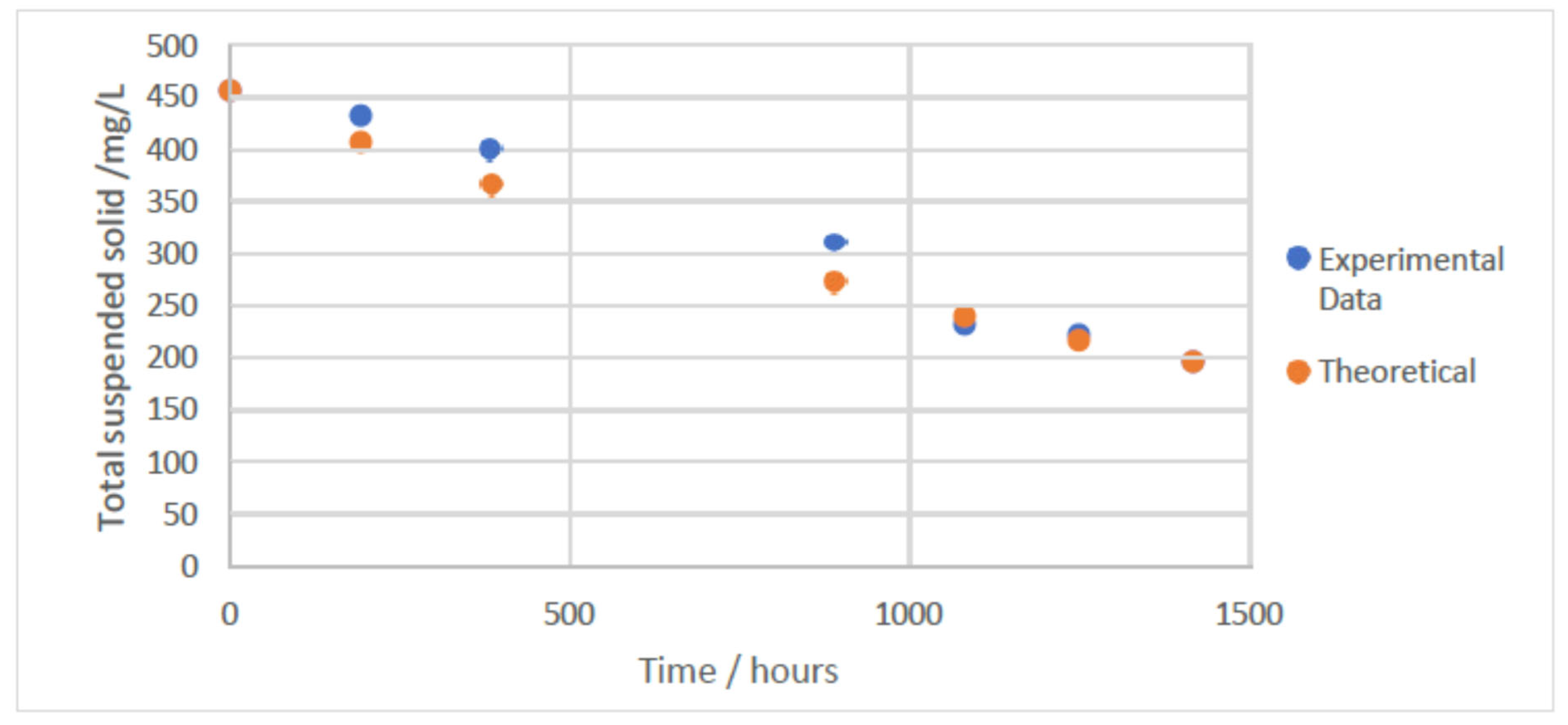
| Total Solids Concentration/mg L−1 | Time/Hr |
|---|---|
| 457 | 0 |
| 433 | 192 |
| 403 | 384 |
| 307 | 888 |
| 233 | 1080 |
| 223 | 1248 |
| 197 | 1416 |
| Changed Parameter | New Value |
|---|---|
| Influent COD concentration | 400 mg COD/L |
| Influent COD concentration | 100 mg COD/L |
| Flow rate | 1.2 L/h |
| Flow rate | 0.4 L/h |
| Parameter in the Default Setting | Value |
|---|---|
| Growth Rate | 1.2 |
| Curvature Min Size | 0.005 mm |
| Curvature Normal Angle | 18.0° |
| Target Skewness | 0.9 |
| Phase Interaction | Drag Coefficient | Lift Coefficient | Turbulent Dispersion | Turbulent Interaction | Virtual Mass Coefficient | Surface Tension Coefficient | Restitution Coefficient |
|---|---|---|---|---|---|---|---|
| Water–AGS | Schiller– Naumann | None | None | None | None | None | - |
| Water–air | Schiller– Naumann | Saffman- mei | None | None | None | None | - |
| AGS–air | Schiller– Naumann | - | - | - | - | None | - |
| AGS–AGS | - | - | - | - | - | - | 0.9 (default constant) |
| Solution Method | ||
|---|---|---|
| Pressure–Velocity Coupling | Scheme | Coupled |
| Spatial Discretization | Gradient | Least Squares Cell Based |
| Pressure | PRESTO! | |
| Momentum | Second-Order Upwind | |
| Volume Fraction | First-Order Upwind | |
| Turbulent Kinetic Energy | First-Order Upwind | |
| Turbulent Dissipation Rate | First-Order Upwind | |
| Transient Formulation | - | First-Order Implicit |
| Dimensionless Parameter | Value |
|---|---|
| Reynolds number air flow | 469 |
| Reynolds number fluid flow | 1.7 |
| Froude number overall flow dynamics | 0.0237 |
| Froude number bubble formation | 0.0531 |
Disclaimer/Publisher’s Note: The statements, opinions and data contained in all publications are solely those of the individual author(s) and contributor(s) and not of MDPI and/or the editor(s). MDPI and/or the editor(s) disclaim responsibility for any injury to people or property resulting from any ideas, methods, instructions or products referred to in the content. |
© 2025 by the authors. Licensee MDPI, Basel, Switzerland. This article is an open access article distributed under the terms and conditions of the Creative Commons Attribution (CC BY) license (https://creativecommons.org/licenses/by/4.0/).
Share and Cite
Siney, M.; Salehi, R.; Hassan, M.G.; Hamza, R.; Shigidi, I.M.T.A. Modelling a Lab-Scale Continuous Flow Aerobic Granular Sludge Reactor: Optimisation Pathways for Scale-Up. Water 2025, 17, 2131. https://doi.org/10.3390/w17142131
Siney M, Salehi R, Hassan MG, Hamza R, Shigidi IMTA. Modelling a Lab-Scale Continuous Flow Aerobic Granular Sludge Reactor: Optimisation Pathways for Scale-Up. Water. 2025; 17(14):2131. https://doi.org/10.3390/w17142131
Chicago/Turabian StyleSiney, Melissa, Reza Salehi, Mohamed G. Hassan, Rania Hamza, and Ihab M. T. A. Shigidi. 2025. "Modelling a Lab-Scale Continuous Flow Aerobic Granular Sludge Reactor: Optimisation Pathways for Scale-Up" Water 17, no. 14: 2131. https://doi.org/10.3390/w17142131
APA StyleSiney, M., Salehi, R., Hassan, M. G., Hamza, R., & Shigidi, I. M. T. A. (2025). Modelling a Lab-Scale Continuous Flow Aerobic Granular Sludge Reactor: Optimisation Pathways for Scale-Up. Water, 17(14), 2131. https://doi.org/10.3390/w17142131