OpenOil-Based Analysis of Oil Dispersion Dynamics: The Agia Zoni II Shipwreck Case

Abstract

This study investigates the spatiotemporal evolution of oil released during the Agia Zoni II shipwreck in the Saronic Gulf in 2017, employing the OpenOil module of the OpenDrift framework. The simulation integrates oceanographic and meteorological data to model the transport, weathering, and fate of spilled oil over a six-day period. Oil behavior is examined across key transformation processes, including dispersion, emulsification, evaporation, and biodegradation, using particle-based modeling and a comprehensive set of environmental inputs. The modeled results are validated against in situ observations and visual inspection data, focusing on four critical dates. The study demonstrates OpenOil’s potential for accurately simulating oil dispersion dynamics in semi-enclosed marine environments and highlights the significance of environmental forcing, vertical mixing, and shoreline interactions in determining oil fate. It concludes with recommendations for improving real-time response strategies in similar spill scenarios.

1. Introduction

The increasing global demand for petroleum products, coupled with diminishing onshore oil reserves, has significantly accelerated the expansion of offshore oil and gas extraction since the 1990s [1]. Simultaneously, advancements in oil transportation—such as the deployment of supertankers and the development of extensive pipeline infrastructures—have enhanced the efficiency of transoceanic oil movement. Despite these technological gains, this upward trend in offshore activity and transport infrastructure has also heightened the risk of accidental oil discharges, posing substantial threats to marine ecosystems and resulting in enduring environmental, social, and economic consequences [1].

Oil spills can originate from various sources, including natural seeps, oil transportation, offshore drilling, and accidents involving vessels, pipelines, or platforms [1]. While smaller spills are generally more manageable and localized, large-scale incidents pose significant challenges in containment and often result in far-reaching environmental damage. Although recent studies indicate a downward trend in the frequency of major oil spills in certain regions—such as the Mediterranean—the public and media tend to focus primarily on high-profile disasters, often overlooking the multitude of smaller, routine spills that occur daily [2]. Data from the International Tanker Owners Pollution Federation (ITOPF) and the European Space Agency reveal that over 80% of recorded oil spill events since 1970 involved quantities under 7 tons [1]. Nonetheless, an estimated 250,000 tons of oil are lost annually during standard shipping operations, with an additional 120,000 tons spilled in proximity to refineries and terminals [1]. Despite these figures, comprehensive data on accidental spills remain scarce or fragmented, underscoring the critical need for more robust oil spill detection and monitoring frameworks.

As shown in

Table 1. Recorded incidents in the Mediterranean Sea.

Date	Location	Oil Spill (tn)
15 May 1966	Sardinia	6000
1 November 1970	Sicily	15,000
11 June 1972	Greece	37,000
25 April 1976	Algeria	31,000
30 June 1976	Greece	15,000
10 August 1977	Bosporus Strait, Turkey	20,000
25 December 1978	Turkey	10,000
2 March 1979	Crete	16,000
15 November 1979	Bosporus Strait, Turkey	64,000
23 February 1980	Navarino Bay, Greece	100,000
29 December 1980	Algeria	37,000
29 March 1981	Corsica	12,200
11 April 1991	Genoa	144,000
30 December 2000	Morocco	9900
14 July 2006	Lebanon	15,000–30,000
10 September 2017	Piraeus, Greece	700–2500
11 February 2021	Lebanon	100–500
Summary
17 cases	Mediterranean Basin	~540,000

, the Mediterranean Sea has experienced numerous large-scale oil spills, with some incidents causing prolonged environmental damage [1]. This historical context is critical for understanding the challenges of managing spills like the Agia Zoni II incident in 2017, which occurred within this sensitive marine region.

The behavior and transformation of oil following a spill are governed by a complex interplay of physical, chemical, and biological processes [3]. Critical factors influencing this evolution include the oil’s composition, oceanographic conditions such as wind, wave dynamics, and currents, as well as the nature of the release—whether abrupt or gradual, and whether it occurs at the surface or from deep-sea sources. Once discharged, oil undergoes a series of weathering processes, including spreading, evaporation, emulsification, dissolution, photo-oxidation, biodegradation, and sedimentation. These processes, in combination with hydrodynamic forces such as mixing, transport, and resurfacing, ultimately dictate the trajectory, persistence, and environmental impact of the spill [3]. Once oil is introduced into the marine environment, it undergoes a series of physical and chemical transformations, beginning with spreading, where the oil forms a thin film over the water’s surface. The speed and extent of this spread depend on environmental factors such as sea surface temperature, oil viscosity, and density [4]. Accurate monitoring of this initial phase is critical for a timely response and impact assessment. In recent years, remote sensing technologies have proven to be essential in oil spill detection and mapping. For instance, object-based image analysis techniques using Sentinel-2 satellite imagery have demonstrated a high effectiveness in identifying both natural oil seeps and recent spill events. A notable application was the detection of a spill along the south coast of Athens, Greece, using Sentinel-2 data, which yielded consistent and promising results for broader implementation [5]. These tools, when combined with traditional modeling approaches, enhance situational awareness during early spill stages and support decision-making for mitigation efforts.

Shipwrecks can lead to substantial oil spills that severely threaten marine and coastal ecosystems. The volume of oil released in such incidents varies depending on the vessel’s cargo and the specific conditions of the wreck, but the environmental consequences can be profound and long-lasting. Historic cases underscore the scale of this threat: the Exxon Valdez disaster in 1989 saw approximately 41 million liters of crude oil discharged into Prince William Sound, Alaska, after the tanker struck a reef, resulting in widespread ecological damage and significant economic losses for local communities [6]. In 2002, the sinking of the Prestige tanker off the coast of Galicia, Spain, released around 13,000 tons of oil into the Atlantic Ocean, affecting marine life and coastlines across both Spain and France [7]. An earlier and equally impactful incident was the Torrey Canyon spill of 1967, when the tanker ran aground near the coast of England, spilling 119,000 tons of crude oil and triggering one of the earliest large-scale oil spill response operations [8]. These events highlight the considerable risks associated with maritime oil transport and emphasize the urgent need for robust prevention strategies and rapid response systems, especially in ecologically sensitive marine regions.

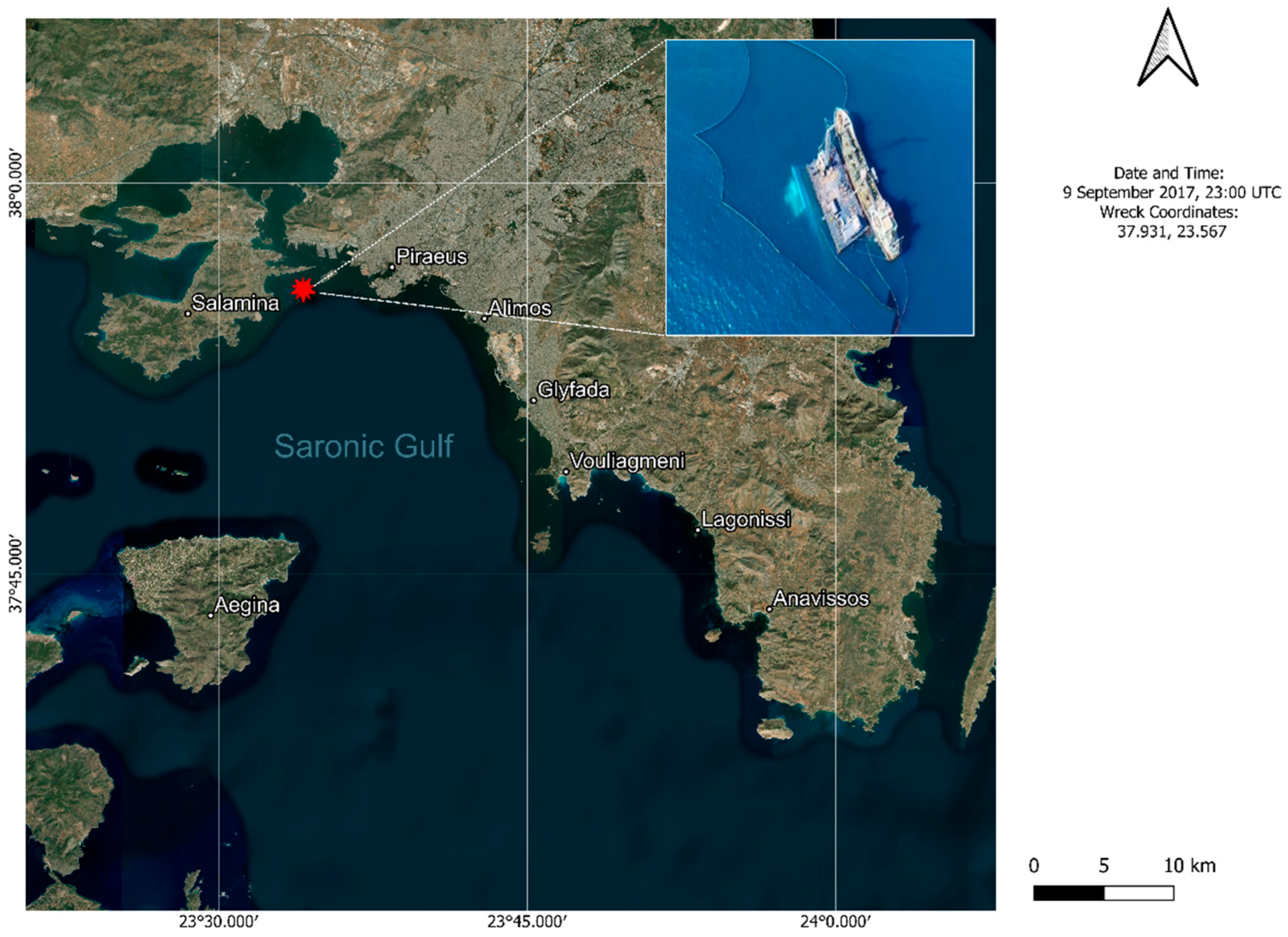
In addition to global examples, regional incidents like the Agia Zoni II shipwreck in the Saronic Gulf, Greece, on 10 September 2017, provide a valuable case study for examining oil spill behavior and response in a semi-enclosed sea. According to the detailed analysis by Gogou et al. [9], this event involved a tanker in relatively good condition that suddenly sank under calm sea conditions, with initial management and containment efforts deployed within the first 24 h. The vessel was carrying significant quantities of oil products, which began leaking into the surrounding waters, contaminating a series of beaches in succession across the coastal zone of Athens. The timeline of the pollution spread, as documented in the study, underscores the dynamic nature of oil dispersion influenced by coastal currents and wind. Pollution status assessments 17 days after the incident revealed persistent contamination in both nearshore waters and sediments. The study also highlights a two-tiered impact: short-term effects such as acute toxicity to marine fauna and beach closures, and long-term consequences including chronic pollution, ecosystem disruption, and socio-economic damage to fisheries and tourism [9].

OpenDrift (Release v1.14.0) is an open-source, Python-based modeling framework developed by the Norwegian Meteorological Institute for simulating particle trajectories in the atmosphere and ocean [10]. Its modular and flexible architecture supports a wide range of applications, including oil spill tracking, search and rescue operations, and biological transport modeling. For example, Hole et al. [11] used OpenDrift with high-resolution data to investigate the 2010 Deepwater Horizon oil spill, demonstrating that river outflows significantly influenced shoreline oiling patterns—underscoring the need to incorporate riverine dynamics into oil spill models. Androulidakis et al. [12] applied OpenDrift over a six-year period to examine oil transport in the Straits of Florida, highlighting the role of large-scale oceanographic features such as the Loop Current. Montaño et al. [13] employed OpenDrift in conjunction with a high-resolution ocean model in New Zealand’s Bay of Plenty, showing that wind-driven upwelling and local wind patterns played a key role in nearshore oil dispersion during 2003–2004.

For this study, the OpenDrift framework’s OpenOil module was employed to simulate the transport and fate of oil released during the Agia Zoni II shipwreck in the Saronic Gulf in 2017. The main goal was to assess OpenOil’s capability in modeling oil spill dynamics in a semi-enclosed marine environment influenced by complex oceanographic conditions and variable atmospheric forcing. The model utilized environmental input data, including ocean currents and wind fields derived from Copernicus Marine Service datasets, to reproduce the observed trajectory and weathering processes of the spill. Calibration and validation efforts were supported by available in situ measurements collected during the response operations, enabling a thorough evaluation of model accuracy and the identification of key factors controlling oil dispersion and persistence in the region.

Overall, special emphasis is given to the following questions:

• How accurately can OpenOil simulate the transport and weathering of oil spills in semi-enclosed marine environments?
• What are the key environmental drivers influencing oil spill dynamics in the Saronic Gulf?
• How can model outputs inform more effective response and long-term management strategies for similar incidents in sensitive coastal zones?

2. Methodology

The methodology section presents the comprehensive framework employed to simulate and analyze the transport and dispersion of oil in the marine environment. It begins with an overview of the OpenOil model, outlining its core features and configuration parameters tailored to this study. Subsequently, the fundamental physical properties and governing equations that drive both horizontal advection and vertical mixing of the oil are described in detail. Following this, the numerical setup specific to the simulation domain—focusing on the Saronic Gulf region impacted by the Agia Zoni II spill—is thoroughly explained.

2.1. OpenOil Model and Its Requirements

This study utilizes the OpenOil module within the OpenDrift framework to simulate the transport and weathering processes of oil released during the Agia Zoni II shipwreck in the Saronic Gulf in 2017. OpenOil combines oil spill transport dynamics with weathering mechanisms by integrating real-time meteorological and oceanographic input data. Operating as a Lagrangian particle-tracking model, it represents the spilled oil as discrete particles, each defined by physical attributes such as mass, viscosity, and density. This particle-based method allows for a detailed and dynamic representation of oil dispersion and transformation in response to the complex environmental conditions of the area [10]. The trajectory of individual oil particles is influenced by ocean current advection, wind-induced drift, and Stokes drift, with a stochastic random walk component included to simulate turbulent diffusion. The key physical processes modeled include wave entrainment [14], turbulence-driven vertical mixing [15], buoyancy-led resurfacing [16], and emulsification [17]. The resurfacing behavior is parameterized based on oil density and droplet size, with sinking velocities calculated using Stokes’ Law, emphasizing the importance of initial droplet size distribution on the overall evolution of the spill [11]. The oil characteristics applied in the model are sourced from the Automated Data Inquiry for Oil Spills (ADIOS) database, which provides comprehensive physical and chemical properties for nearly 1000 different oil types globally. This extensive dataset ensures a realistic simulation of oil weathering processes within the model framework [18].

This study uses the Mediterranean Multi-Year Physical Reanalysis (Med MFC) product, produced by a coupled numerical system consisting of the NEMO hydrodynamic model and OceanVAR variational data assimilation for temperature, salinity, and satellite sea level anomaly data. The dataset includes a reanalysis and an interim dataset extending to one month before the present. The Med MFC model features a high horizontal resolution of 1/24° (~4–5 km) and 141 uneven vertical levels, offering detailed ocean physical state variables. These data support the simulation by providing accurate ocean conditions such as temperature, salinity, currents, and sea level [19].

The MEDSEA_MULTIYEAR_WAV_006_012 product provides a multi-year reanalysis of Mediterranean Sea waves starting from 1985, with hourly wave parameters at a 1/24° (~4–5 km) resolution. It includes a reanalysis dataset, an interim dataset up to one month before the present, and a monthly climatology (1993–2016). The Med-WAV system uses the WAM 4.6.2 wave model with a nested grid setup, covering the North Atlantic and Mediterranean Sea to capture swell propagation through the Strait of Gibraltar. The model resolves wave spectra across 24 directions and 32 frequency bins and assimilates the satellite observations of significant wave heights. Forcing data includes daily averaged ocean currents and high-resolution ERA5 wind fields at 10 m above sea level [20].

ERA5 is the fifth-generation global climate and weather reanalysis from ECMWF, providing data from 1940 onwards and succeeding the ERA-Interim dataset. It combines numerical model outputs with worldwide observations through data assimilation to create a consistent, physics-based estimate of atmospheric conditions over time. Unlike real-time forecasts, ERA5 benefits from extensive observation integration, allowing for improved accuracy, especially for historical periods. This study uses ERA5 hourly single-level data aggregated to daily statistics, including options for daily mean, max, min, and sums, with flexibility for sub-daily sampling and local time zone adjustments [21].

2.2. Physical Properties and Governing Equations

The simulation of oil transport accounts for key physical processes that govern how oil moves and spreads in the ocean. These include both horizontal and vertical transport mechanisms, which together describe the movement of oil particles in the water column.

2.2.1. Horizontal Transport

Oil particles move horizontally under the influence of ocean currents, wind, and wave-induced Stokes drift. These factors affect both surface and submerged oil. Wind drift typically contributes around 3% of the wind speed at 10 m height, though values can range from 1% to 6% [22]. Stokes drift is included based on the method developed by Breivik et al. [23], using the Phillips wave spectrum.

2.2.2. Vertical Transport

(a) Wave Entrainment: Breaking waves can force oil droplets from the surface into the water column, especially during storms. This mixing process depends on oil properties (such as viscosity and surface tension), wave energy, and environmental conditions [24]. The fraction of the sea surface affected by wave breaking (F_bw) increases with the wind speed and wave period and is calculated as follows:

$$F_{bw}=\left\{\begin{array}{c}{a}_{bw}{\displaystyle \frac{U_{10\mathrm{m}}-U_o}{T_p}} if{U}_{10\mathrm{m}}>U_o\\ 0 if{U}_{10\mathrm{m}}\le U_o\end{array}\right.$$

(1)

where α_bw = 0.032 s/m (constant), U_10m is the wind speed at 10 m above sea level, U_o is the minimum wind speed that starts wave breaking (considered equal to 5 m/s), and T_p is the significant wave period taken from the wave data.

The rate of vertical oil flux Q is given by the following:

$$Q=4.604\times {10}^{-10}{We}^{1.805}{Oh}^{-1.023}{F}_{bw}$$

(2)

where We is the Weber number, representing inertial vs. surface tension forces, and Oh is the Ohnesorge number, representing viscous effects. These are calculated using wave height, oil properties, and the Rayleigh–Taylor instability diameter d_o, which estimates the breakup size for droplets in wave conditions [22].

(b) Oil Resurfacing: Due to buoyancy, oil droplets rise through the water. Their upward speed depends on size and density contrast with seawater. Small droplets follow Stokes’ law, while larger ones use a Reynolds-based approach [16,25]. For instance, a 0.01 mm droplet might rise at 1 cm/h, while a 0.5 mm droplet can ascend at 30 m/h [20].

(c) Oil Droplet Size Distribution: When oil is released at depth, droplets form in a range of sizes, typically between 0.1 mm and 0.5 mm [26]. Their size affects how quickly they rise and how far they are carried by underwater currents. The droplet size follows a lognormal distribution, with the median diameter D₅₀^V:

$$D_{50}^V=d_o{r}_e{\left(1+10Oh\right)}^p{We}^q$$

(3)

where r_e = 1.791, p = 0.46, and q = −0.518 are empirical constants [25]. The probability density function (PDF) of the droplet size is as follows:

$$PDF={\displaystyle \frac{1}{ds\sqrt{2\pi }}}exp\left({\displaystyle \frac{-{\left(lnd-ln{D}_{50}^V\right)}^2}{2s^2}}\right)$$

(4)

where s = 0.38, the standard deviation of the distribution [22]. The volume distribution follows a power-law:

$$V\left(d\right)=d^{-0.7},d\epsilon \left[d_{min},d_{max}\right]$$

(5)

where d ranges from 1 µm (10⁻⁶ m) to 1 mm (10⁻³ m).

(d) Turbulent Mixing: Vertical turbulence also helps redistribute oil in the water column. This mixing is influenced by wind, wave energy, and water stratification. It is represented by the vertical diffusivity coefficient K(z), and oil particle movement is calculated using a random walk method [27]. The vertical displacement Δz over time Δt is as follows:

$$\Delta z=K^{\prime }\left(z_n\right)\Delta t+R\sqrt{{\displaystyle \frac{2}{r_s}}K\left(z_n+{\displaystyle \frac{K^{\prime }\left(z_n\right)\Delta t}{2}}\right)\Delta t}$$

(6)

where K′(z_n) is the vertical gradient of diffusivity, R is a random number (mean = 0), and r_s is the variance scaling factor.

2.3. Oil Weathering Processes

OpenOil incorporates advanced models for key oil weathering processes: (a) dispersion, (b) evaporation, (c) emulsification, and (d) biodegradation. These processes use oil property data from NOAA’s ADIOS Oil Library. Evaporation rates vary widely depending on oil type and environmental factors like wind speed [22]. Evaporation and emulsification significantly change oil density, viscosity, and interfacial tension, which influence droplet size distribution [11].

(a) Dispersion: Dispersion describes how oil droplets are mixed into the water column by turbulence generated by wind and waves [22]. OpenOil applies the Delvigne and Sweeney method [28], estimating wave energy dissipation as follows:

$$D_e=0.0034\times g{\rho }_{sw}{H}_s^2$$

(7)

where ρ_sw is the seawater density (1028 kg/m³), g is gravity (9.81 m/s²), and H_s is the significant wave height (taken from wave data).

The dispersion coefficient (c_disp) quantifies how much of this energy contributes to oil dispersion:

$$c_{disp}={\left(D_e\right)}^{0.57}{f}_{bw}$$

(8)

where f_bw (the fraction of breaking waves) is set to 0.02.

The oil dispersion rate into the water column (q_disp) is then computed as follows:

$$q_{disp}={\displaystyle \frac{c_{Roy}{c}_{disp}{V}_{entrain}}{{\rho }_{oil}}}$$

(9)

where $c_{Roy}=2400\times exp\left(-73.682\times \sqrt{{\displaystyle \frac{{\mu }_{oil}}{{\rho }_{oil}}}}\right)$ is Roy’s constant, accounting for the oil’s viscosity and density effects, and V_entrain = 3.9 × 10⁻⁸ m³/s is the entrainment volume constant per second, μ_oil = 1.057 cPoise is the dynamic viscosity, and ρ_oil = 938.0 kg/m³ is the density of the generic heavy crude oil.

(b) Evaporation: OpenOil adapts evaporation modeling to slick conditions [22]. In calm seas, Stiver and Mackay’s analytical model is used [29]. Under rough conditions, the model switches to ADIOS2’s pseudo-component approach, representing oils as several non-interacting components, each with unique vapor pressures. Vapor pressures are estimated from molar volumes, linked to alkane boiling points, using Antoine’s equation [30].

(c) Emulsification: Emulsification is modeled after Lehr et al. [18], considering oil weathering, evaporation, water content, and droplet size distribution. The oil–water interfacial area S grows over time, driven by wave energy and wind, but is capped at a maximum S_max = 5.4 × 10⁷ m². The water fraction Y in the emulsion evolves as follows:

$$Y={\displaystyle \frac{S{d}_w}{6+S{d}_w}}$$

(10)

where d_w is the average water droplet diameter.

(d) Biodegradation: Biodegradation was represented using a first-order decay model with distinct half-lives for surface slicks and subsurface droplets [31]. This approach assumes that the degradation of oil over time follows an exponential decay function, described by the following:

$$C\left(t\right)=C_0·exp\left(-k_{d}t\right)$$

(11)

where C(t) is the remaining oil mass at time t (days), C₀ is the initial oil mass (kg), and k_d is the decay rate constant (day⁻¹). The decay constant is related to the half-life (t_1/2) by the following equation:

$$k_d={\displaystyle \frac{ln2}{t_{1/2}}}$$

(12)

For the purposes of this study, the half-life of surface slicks was set to 3 days, yielding a decay constant of approximately k_d = 0.231 day⁻¹, while the half-life for dispersed droplets was set to 1 day, corresponding to k_d = 0.693 day⁻¹ [32]. These values were applied independently to the respective oil phases in the simulation to dynamically estimate mass loss due to microbial degradation over time. This formulation offers a simplified yet effective representation of natural biodegradation, which is influenced by environmental factors such as hydrocarbon type, water temperature, microbial activity, oxygen availability, and nutrient levels [31].

2.4. Simulation Setup and Study Area

The Saronic Gulf is situated in the west-central Aegean Sea, bordered by the Attica Peninsula to the north and east and the Peloponnese to the southwest. It connects to the wider Aegean Sea to the south and southeast and features numerous islands and islets, notably Salamina and Aegina. The gulf spans approximately 270 km of coastline and encompasses a sea surface area of around 2890 km², with an average water depth of roughly 100 m [33]. The eastern coastline of the gulf, particularly along the Attica region, is home to several popular and ecologically sensitive beaches, including Alimos, Glyfada, Vouliagmeni, Lagonissi, and Anavissos, many of which are key recreational and tourism hubs (Figure 1) and are potentially vulnerable to oil contamination in the event of a spill [9].

This study focuses on simulating the Agia Zoni II oil spill, which occurred on 9 September 2017 at 23:00 UTC, near Piraeus Harbor, one of the busiest ports in the Eastern Mediterranean. The oil release was simulated using the OpenOil model, incorporating high-resolution environmental forcing datasets, including wind fields, ocean currents, salinity, temperature, wave velocity, and bathymetry, sourced from the Copernicus Marine Environment Monitoring Service (CMEMS) and GSHHG landmask data.

A total of 42,000 oil particles were seeded within a 20 m radius spill zone, centered at longitude 23.567° E and latitude 37.931° N, approximately 5 m below the sea surface. The release spanned 84 h—from 9 September at 23:00 UTC to 13 September at 11:00 UTC—with a continuous discharge rate of 2.157 m³/h, resulting in a total spill volume of approximately 181.19 m³, equivalent to roughly 170 metric tons. The overall simulation continued until 15 September 2017 at 11:00 UTC. The release end date of 13 September was deliberately chosen to coincide with the reported deployment of the Aktea vessel by the European Maritime Safety Agency (EMSA), which supported decontamination operations following the spill. On the same day, the Hellenic Ministry of Shipping and Island Policy formally notified both the European Commission and the Secretariat of the Barcelona Convention for the Mediterranean—marking a critical escalation in international response and coordination efforts [9]. The oil type used in the simulation was “GENERIC HEAVY CRUDE,” with an assumed density of 938 kg/m³, a kinematic viscosity of 1.127 × 10⁻⁶ m²/s at 20 °C, and a lognormal droplet size distribution ranging from 1 μm to 3 mm, based on the parameterization of Li et al. [34].

The model configuration accounted for multiple oil weathering processes, including evaporation, emulsification, dispersion, biodegradation, and coastline stranding. Vertical mixing and Stokes drift were also activated, enhancing realism in particle behavior and subsurface transport. Biodegradation was modeled using a half-time approach, with slick and droplet half-lives set at 3 and 1 days, respectively. Wind drift factors varied randomly between 0% and 6% to capture variability in surface transport.

Table 2. Simulation configurations: parameters and settings used in the oil spill model.

Purpose	Examination
Study Area	Saronic Gulf, Mediterranean, Agia Zoni II shipwreck
Date start (UTC)	9 September 2017, 23:00 UTC
Geographical Coordinates	23.567° E, 37.931° N
Oil Type	Generic heavy crude
Discharge Rate	2.157 m3/h
Particle Release Rate	500 particles/h
Total Seeding Elements	42,000
Seeding Radius	20 m
Oil Spill Duration	84 h (continuous spill)
Droplet Size Distribution	1 μm–3 mm
Wind Drift Factors	0–6%
Processes Considered	Evaporation, emulsification, dispersion, biodegradation, wind drift, vertical mixing, wave entrainment, and coastline stranding
Simulation Duration	132 h (hourly outputs) in a NetCDF file

summarizes the environmental inputs and model configurations applied in the simulation.

3. Results

The simulation reconstructed the transport and weathering processes of oil released from the Agia Zoni II shipwreck, which occurred on 9 September 2017, in the Saronic Gulf. The model tracks the behavior of the spilled oil over a period spanning 10 to 15 September 2017, under the combined influence of ocean currents, wind forcing, and environmental conditions representative of that time. As the oil drifted, it underwent a range of fates: dispersal into the water column, surface spreading, shoreline stranding, or submersion, with each pathway affected by hydrodynamic conditions and oil weathering processes. The simulation accounted for key physical and chemical changes in the oil, including droplet size distribution, emulsion formation, viscosity evolution, and water uptake. To align with available in situ measurements and field observations, the analysis focuses on four critical dates: 10, 12, 14, and 15 September 2017. These snapshots provide insight into the spatial distribution and transformation of the oil, supported by quantitative metrics, weathering statistics, and comparative assessments between modeled and observed outcomes.

In Figure 2, the top-left panel (Figure 2a) presents the volume spectrum, illustrating a right-skewed distribution where most of the oil volume is concentrated in droplets with diameters around 0.0005 to 0.0015 m, though a long tail persists toward larger droplets. This highlights that larger droplets, while fewer, significantly contribute to the total dispersed volume. The top-right panel (Figure 2b) shows the cumulative volume spectrum, which confirms that the bulk of the oil volume accumulates at smaller droplet diameters, indicating the predominance of fine droplets in the volume budget. In the middle row, the number spectrum (Figure 2c) displays a strong peak at very small droplet sizes, with a steep decline toward larger diameters. The OpenOil result (blue) indicates a more irregular distribution with multiple peaks compared to the smoother, monotonic curve from Li et al. [34] (orange), suggesting either higher resolution or variability in the modeled breakup dynamics. The cumulative number spectrum (Figure 2d) reinforces this observation, with over 80% of droplets below ~0.0005 m. However, the OpenOil result shows a more gradual rise compared to the steeper empirical curve, indicating a broader distribution of droplet sizes in the model. The bottom row provides logarithmic representations. The log number spectrum (Figure 2e) reveals a characteristic decay trend, but with small deviations, possibly due to the numerical resolution in the model. In contrast, Li et al.’s [34] distribution maintains a smoother log-linear decay. The log cumulative number spectrum (Figure 2f) demonstrates a near-linear ascent for both datasets, though the slope differs, again reflecting the broader spread of droplet sizes predicted by the simulation. These comparisons highlight the OpenOil model’s capability to reproduce the general statistical behavior of oil droplet distributions under turbulent marine conditions, while also revealing potential differences in fragmentation modeling or parameter sensitivity. Understanding these distributions is vital for assessing oil fate processes such as dispersion, emulsification, and vertical transport in the water column.

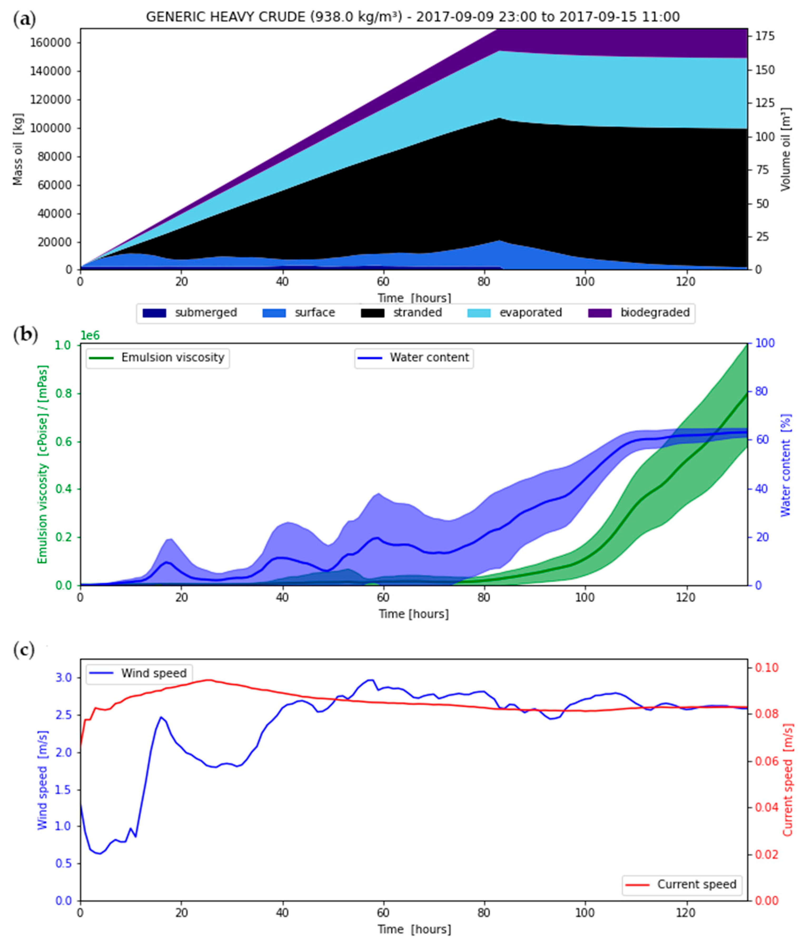
Oil budget evolution and weathering characteristics were simulated for generic heavy crude (938.0 kg/m³) over a period of 132 h (from 9 September 23:00 UTC to 15 September 11:00 UTC), representing conditions following the Agia Zoni II oil spill. The top panel (Figure 3a) illustrates the time evolution of oil mass partitioned among key fate processes: dispersed, submerged, surface-resident, stranded, evaporated, and biodegraded. Early in the simulation, a substantial portion of the oil accumulates on the surface and rapidly transitions to the stranded category, indicating significant shoreline interaction. By around hour 100, the stranded mass plateaus, dominating the oil budget. The evaporated fraction increases steadily but remains modest relative to stranded and surface-bound oil. Submerged and dispersed fractions remain minor throughout, suggesting low mixing energy or a tendency for the heavy crude to resist vertical entrainment. Biodegradation becomes noticeable only in the final stages of the simulation, with a slow but consistent rise in mass, indicating the onset of biological transformation processes. The middle panel (Figure 2b) shows the evolution of two key weathering parameters: emulsion viscosity (green shaded area) and water content (blue shaded line), both of which increase markedly in the final third of the simulation. Water content surpasses 60% after 100 h, stabilizing near that level, while emulsion viscosity climbs sharply in the last 24 h to values exceeding 9 × 10⁵ cPoise/mPa·s, characteristic of a highly viscous, water-in-oil emulsion. The shaded regions suggest spatial variability, likely resulting from differing exposure conditions (wave energy, oil patch size). The bottom panel (Figure 3c) depicts wind speed (blue line, left axis) and current speed (red line, right axis). Wind speed remains variable but generally stays within 1.5 to 3 m/s, which is sufficient to induce surface agitation and potentially facilitate emulsification. Current speed shows a mild downward trend, decreasing from just above 0.09 m/s to about 0.08 m/s, suggesting weak horizontal transport forces. These relatively low environmental energy conditions contribute to the dominance of surface accumulation and shoreline stranding, with limited dispersion or vertical entrainment. Overall, the simulation indicates that under the environmental conditions specific to the Agia Zoni II timeframe, the oil primarily becomes stranded or remains at the surface, with slow weathering, high emulsification, and minimal biodegradation over the modeled period.

Sentinel-1A and 1B SAR imagery was initially considered for identifying the oil spill caused by the Agia Zoni II incident. However, due to very low wind speeds (Figure 3) in the days following the sinking, the resulting SAR images displayed extensive dark areas that could not be reliably attributed to oil slicks. Consequently, these images were not used in the present analysis. Additionally, they are not shown here, as they have already been thoroughly analyzed and discussed in the work by Kolokoussis and Karathanassi [5].

Following the initial particle release depicted in Figure 4a, the oil droplets experience a rapid descent to a mean depth exceeding −5 m, consistent with an early submergence event. Over the next 24 h, particles exhibit a gradual upward migration, stabilizing around −1 to −0.5 m, and progressively approaching the surface by the end of the simulation period. Figure 4b presents the mean depth evolution (z) of oil particles over time, covering the period from the early morning of 10 September 2017 through 15 September 2017, based on the OpenOil simulation of the Agia Zoni II oil spill. These modeled results are consistent with the incident response timeline described in [9]. At 06:00 on 10 September, anti-pollution vessels of the Hellenic Coast Guard arrived on site. Simultaneously, the Ministry of Shipping and Island Policy reported that private contractors had been mobilized for ship sealing and decontamination, and the Local Contingency Plan of Piraeus and the Saronic Gulf was activated. Despite the rapid deployment of resources, the first floating barriers were installed two hours after the full immersion of the vessel. By then, a significant fraction of petroleum products had already escaped, likely due to vertical mixing and subsurface transport beyond the 1 m draft limit of the containment booms, exacerbated by the prevailing meteorological conditions. On the morning of 11 September, the Ministry of Environment and Energy officially characterized the situation as “very special,” initiating the Independent Coordination Office for the Implementation of Environmental Liability. Environmental Inspectors were deployed in the field, while both the European Commission and the Secretariat of the Barcelona Convention were notified. On 13 September, the response was further supported by the Aktea vessel of the European Maritime Safety Agency (EMSA). The simulation shown in Figure 4b substantiates field observations by demonstrating the initial subsurface retention of oil and the delayed surfacing of the plume, factors that critically impacted the efficacy of early containment measures. This underscores the importance of immediate deep-column monitoring and response coordination during oil spill events, especially under dynamic weather conditions.

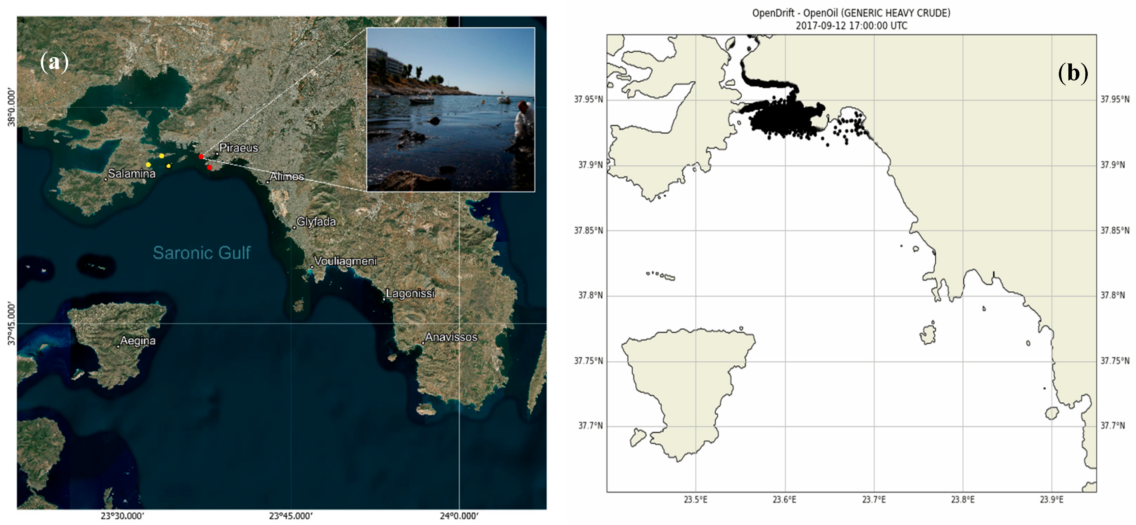
A comparative analysis was conducted between observed oil spill locations and OpenOil model simulations for four key dates following the Agia Zoni II incident. For each date, two visual datasets were examined: (a) in situ observations indicating confirmed surface oiling, marked by red dots based on data from [9], and (b) the corresponding distribution of simulated oil particles produced by the OpenOil model at the same timestamp.

To support a more detailed evaluation of oil particle trajectories, a custom Python-based analysis tool was incorporated into the OpenOil module (see Supplementary Material). This tool enabled the extraction of essential kinematic indicators—including Mean Direction (in degrees), Dominant Compass Direction, Mean Speed (excluding stationary particles), and Mean Travel Distance—providing deeper insight into transport dynamics and spatial dispersion patterns.

Table 3. Summary of simulated oil particle transport characteristics.

Date	Time	Mean Direction (°)	Compass Direction	Mean Speed (m/s)	Mean Distance (m)
10 September 2017	11 UTC	8.998	N	0.092	1666.89
12 September 2017	17 UTC	50.264	NE	0.137	2786.88
14 September 2017	11 UTC	92.276	E	0.130	4787.59
15 September 2017	11 UTC	117.231	SE	0.126	5235.22

summarizes the computed values for each of the four analyzed dates, offering a quantitative perspective on particle transport behavior in relation to the observed oiling patterns.

The 1st key date—10 September 2017 11 UTC: Figure 5 represents the initial stages of the spill, approximately one day after the Agia Zoni II sank. In situ observations show localized surface oiling primarily concentrated near the wreck site, close to Piraeus and the southeastern coast of Salamina. The simulation successfully replicates this early-stage concentration, with particle clustering evident within a 1–3 km radius from the source point. The modeled dispersion appears consistent with the weak current and wind activity observed during this period. No significant offshore transport is detected, suggesting a dominant influence of local eddies and limited wave energy on dispersion. Quantitative analysis of particle trajectories for this date supports these observations. The mean movement direction was calculated as 8.998°, corresponding to a northerly (N) compass heading. The mean transport speed of the particles, excluding stationary ones, was 0.092 m/s, while the average travel distance from the source was 1666.89 m. These values confirm the limited spread and slow transport of the oil in the immediate aftermath of the incident.

The 2nd key date—12 September 2017 17 UTC: By this date, the in situ observations show a broader spread of surface oil extending southwest along the coast of Salamina and towards the western shoreline of the Athens Riviera. The OpenOil model captures this west–southwest drift pattern effectively. Simulated particles show significant stranding along the Salamina coastline and some encroachment towards Paloukia and Perama (Figure 6). This agreement highlights the model’s ability to integrate localized coastal currents and prevailing wind directions, which played a critical role in this phase of transport. The increasing oil–water interaction processes, such as emulsification and initial dispersion, are reflected in the broader simulation footprint. Quantitative outputs for this date further support the observed transport dynamics. The computed mean movement direction was 50.264°, corresponding to a northeast (NE) compass heading, indicative of the complex flow dynamics near the stranding zones. The mean particle speed was 0.137 m/s, and the average distance traveled reached 2786.88 m. These values reflect increased particle mobility and dispersion relative to the initial spill stages, consistent with the expanding spatial impact observed in the field.

The 3rd key date—14 September 2017 11 UTC: By 14 September, in situ data indicate widespread contamination reaching areas further south, including portions of the Athens Riviera, notably near Elliniko, Alimos, and Glyfada. The OpenOil simulation predicts this expanded trajectory, showing a bifurcated plume pattern: one part continues southwestward, while another fragment drifts southeast due to shifting wind directions (Figure 7). Particle density diminishes further from the source, indicating ongoing weathering and partial biodegradation. The model successfully simulates stranded elements along the coastline, consistent with the reported beach pollution and the containment challenges encountered during cleanup efforts. Supporting these observations, the quantitative analysis reveals a mean movement direction of 92.276°, corresponding to an easterly (E) compass heading. The mean particle speed was 0.130 m/s, with an average travel distance of 4787.59 m, reflecting a notable increase in both the dispersion range and transport velocity compared to earlier stages. These metrics corroborate the more extensive spatial distribution and complex plume dynamics observed on this date.

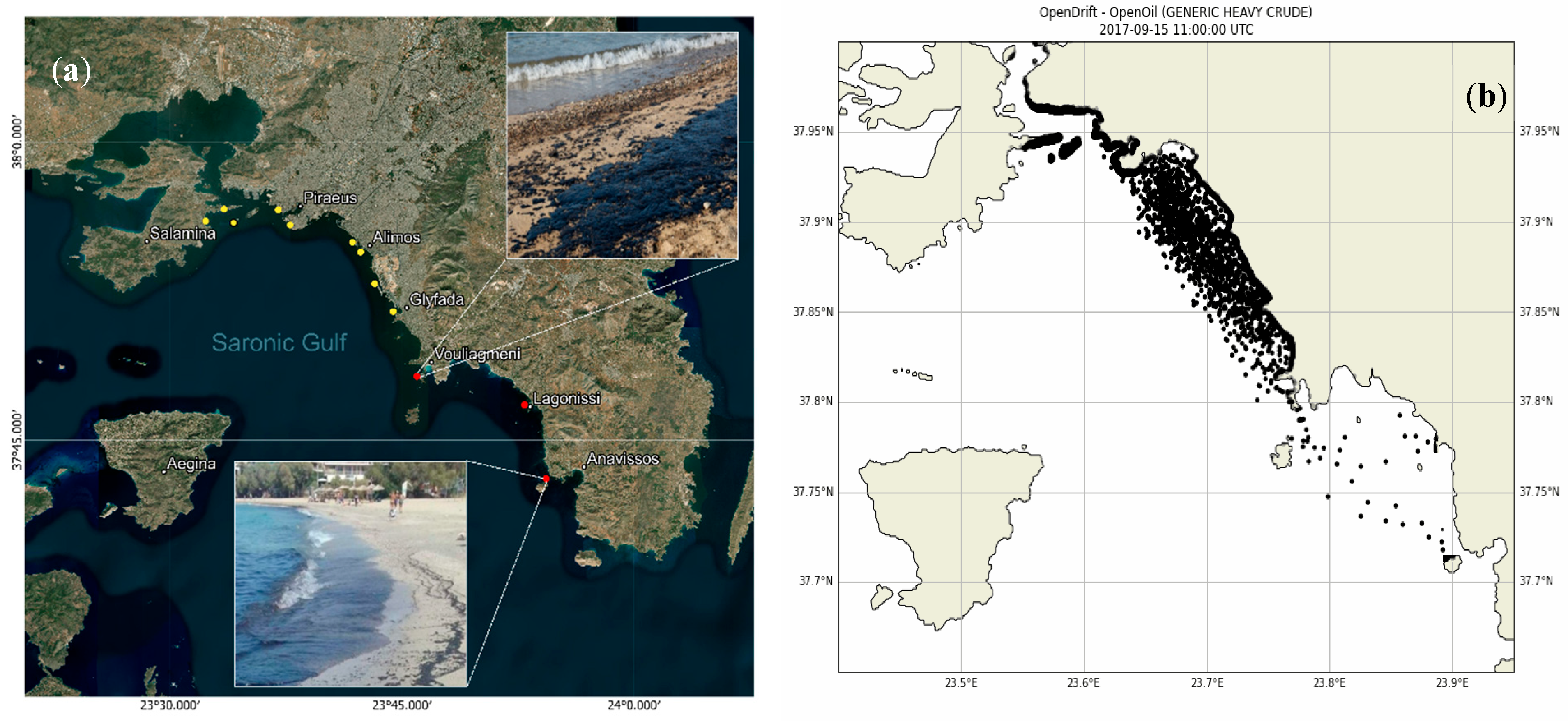
The 4th key date—15 September 2017 11 UTC: On the final analyzed date, in situ observations confirm persistent pollution along the southern Attica coast, particularly around the beaches of Vouliagmeni, Lagonissi, and Anavissos. The OpenOil simulation mirrors this, showing stranded oil particles detected along the entire southeastern coastline. The model suggests that while the active offshore transport of oil diminished, localized recirculation and surf zone entrainment maintained the shoreline contamination (Figure 8). This is corroborated by visual reports and response efforts documented by authorities. The convergence between modeled and observed locations emphasizes the value of OpenOil in reproducing both nearshore and coastal stranding behavior even several days post-incident. Quantitative trajectory analysis supports this interpretation, with a mean particle movement direction of 117.231°, corresponding to a southeast (SE) compass heading. The mean speed was 0.126 m/s, and the average distance traveled increased to 5235.22 m, indicating continued particle mobility primarily confined to nearshore transport mechanisms. These findings reinforce the persistence of shoreline contamination driven by localized hydrodynamic processes during the late phase of the spill.

4. Conclusions

This study presents a detailed simulation of the Agia Zoni II oil spill in the Saronic Gulf using the OpenOil model, emphasizing the dynamic interplay between environmental forcing, oil weathering processes, and physical transport mechanisms. The following key conclusions were drawn:

(1) Simulation accuracy and validation: The OpenOil model successfully reproduced the main dispersion and stranding patterns observed during the Agia Zoni II incident. Comparisons with in situ data for four key dates showed strong spatial correspondence, particularly in predicting shoreline contamination in high-risk zones such as Salamina and the southern Attica coastline.

To enhance this comparison, a Python-based analytical tool was integrated into the OpenOil module (see Supplementary Material), enabling the extraction of key kinematic variables: Mean Direction (in degrees), Dominant Compass Direction, Mean Speed (excluding stationary particles), and Mean Travel Distance. These metrics facilitated a more nuanced evaluation of oil particle behavior and spatial patterns.

(2) Dominance of shoreline stranding: Under the prevailing low-energy environmental conditions—characterized by weak wind and current speeds—the primary fate of spilled oil was stranding along the coastline. This was evident in the early mass accumulation in the “stranded” category and the stagnation of offshore movement beyond 13 September 2017.

(3) Vertical dynamics and delayed surfacing: The simulation captured the initial submersion of oil particles, followed by a gradual ascent toward the surface over time. This behavior, consistent with field observations, suggests that early containment efforts were compromised by vertical mixing processes that moved oil below the draft level of the booms.

(4) Weathering and emulsification trends: Oil weathering metrics indicated rapid emulsification during the later stages of the simulation, with viscosity and water content peaking after 100 h. This transformation rendered the oil more persistent and difficult to disperse, highlighting the importance of timely mechanical recovery efforts before emulsification sets in.

(5) Biodegradation modeling approach: The first-order decay model with phase-specific half-lives (3 days for slicks and 1 day for droplets) provided a simple yet effective method to represent microbial degradation. However, biodegradation contributed modestly to mass reduction within the modeled timeframe, implying a limited short-term role in environmental cleanup.

(6) Sentinel-1 limitations and data integration: Sentinel-1 SAR imagery, though initially considered, proved ineffective due to low wind conditions, reaffirming the importance of integrating multiple observational sources for spill detection. The exclusion of these images from this study was justified, given their prior analysis in the existing literature.

(7) Operational utility of OpenOil: The model proved to be a valuable decision-support tool, capable of capturing the evolution of oil spill events in complex coastal environments. Its predictive capability supports not only retrospective analysis but also real-time forecasting for emergency response.

Beyond its case-specific relevance, this study demonstrates how the OpenOil framework can serve as a transferable tool for simulating oil dispersion in other semi-enclosed or complex marine environments. The insights into oil weathering dynamics, subsurface transport, and shoreline stranding behavior are broadly applicable to similar spill scenarios, especially in regions with limited energy input and sensitive coastal infrastructure. The model’s ability to replicate observed spill trajectories and transformation processes underlines its potential as a decision-support asset for environmental managers, response teams, and policy makers. By integrating environmental data and accounting for multiple oil transformation pathways, the approach adopted here contributes to the development of reliable, generalizable methodologies in environmental modeling and software for marine pollution management.

The results of this study offer practical value for coastal spill response planning and environmental management. By accurately capturing the timing and extent of shoreline stranding, the OpenOil model can support the prioritization of response actions in high-risk areas, especially during the early hours of a spill event. The identification of vertical mixing and delayed surfacing as critical transport mechanisms highlights the need for containment strategies that extend below the surface layer, beyond the draft depth of conventional booms. Additionally, the simulation underscores the importance of timely mechanical recovery before significant emulsification occurs, informing operational windows for effective cleanup. These findings can guide environmental authorities, contingency planners, and port managers in refining preparedness protocols, optimizing resource allocation, and updating local contingency plans for oil spill incidents. More broadly, integrating such modeling tools into decision-support systems enhances the scientific basis for emergency response, strengthens inter-agency coordination, and supports compliance with regional marine protection frameworks

In summary, this work underscores the importance of rapid modeling integration in oil spill scenarios, particularly in semi-enclosed, ecologically sensitive basins like the Saronic Gulf. Future work should explore ensemble modeling approaches, improved remote sensing integration, and longer-term tracking of biodegradation and sedimentation processes to further strengthen the role of environmental modeling in operational spill response and marine system management such as the Barcelona Convention.

References

1. ITOPF. Oil Tanker Spill Statistics 2023; ITOPF: London, UK, 2024; Available online: https://www.itopf.org/knowledge-resources/data-statistics/statistics/ (accessed on 14 January 2025).
2. Carpenter, A.; Kostianoy, A.G. Oil pollution in the Mediterranean Sea: Part I: The international context. In The Handbook of Environmental Chemistry; Barceló, D., Kostianoy, A.G., Eds.; Springer: Berlin/Heidelberg, Germany, 2018; Volume 83. [Google Scholar] [CrossRef]
3. Papaioannou, V.; Anagnostopoulos, C.G.E.; Mantsis, D.F.; Vlachos, K.; Moumtzidou, A.; Gialampoukidis, I.; Vrochidis, S.; Kompatsiaris, I. Assessment of oil spill dispersion and weathering processes in Saronic Gulf. Adv. Hydrol. Meteorol. 2025, 2, 000550. [Google Scholar] [CrossRef]
4. Simecek-Beatty, D.; Lehr, W.J. Extended oil spill spreading with Langmuir circulation. Mar. Pollut. Bull. 2017, 122, 226–235. [Google Scholar] [CrossRef] [PubMed]
5. Kolokoussis, P.; Karathanassi, V. Oil spill detection and mapping using Sentinel 2 imagery. J. Mar. Sci. Eng. 2018, 6, 4. [Google Scholar] [CrossRef]
6. Jewett, S.; Dean, T.A.; Smith, R.O.; Blanchard, A. ‘Exxon Valdez’ oil spill: Impacts and recovery in the soft-bottom benthic community in and adjacent to eelgrass beds. Mar. Ecol. Prog. Ser. 1999, 185, 59–83. [Google Scholar] [CrossRef]
7. Albaigés, J.; Bernabeu, A.; Castanedo, S.; Jiménez, N.; Morales-Caselles, C.; Puente, A.; Viñas, L. The Prestige oil spill. In The Handbook of Environmental Chemistry; Wiley Online Library: New York, NY, USA, 2014; pp. 513–545. [Google Scholar] [CrossRef]
8. Cooper, T.; Green, A. The Torrey Canyon disaster, everyday life, and the ‘greening’ of Britain. Environ. Hist. 2017, 22, 26–47. [Google Scholar] [CrossRef]
9. Gogou, M.; Antoniades, C.; Andreadakis, E.; Chalvantzi, E.; Lekkas, E.; Perrou, D.; Parcharidis, I. Agia Zoni II shipwreck, Saronic Gulf, 10 September 2017. Newslett. Environ. Disaster Crises Manag. Strateg. 2017, 4, 1–26. [Google Scholar]
10. Dagestad, K.-F.; Röhrs, J.; Breivik, Ø.; Ådlandsvik, B. OpenDrift v1.0: A generic framework for trajectory modelling. Geosci. Model. Dev. 2018, 11, 1405–1420. [Google Scholar] [CrossRef]
11. Hole, L.R.; Dagestad, K.-F.; Röhrs, J.; Wettre, C.; Kourafalou, V.H.; Androulidakis, Y.; Kang, H.; Le Hénaff, M.; Garcia-Pineda, O. The DeepWater Horizon oil slick: Simulations of river front effects and oil droplet size distribution. J. Mar. Sci. Eng. 2019, 7, 329. [Google Scholar] [CrossRef]
12. Androulidakis, Y.; Kourafalou, V.; Hole, L.R.; Le Hénaff, M.; Kang, H. Pathways of Oil Spills from Potential Cuban Offshore Exploration: Influence of Ocean Circulation. J. Mar. Sci. Eng. 2020, 8, 535. [Google Scholar] [CrossRef]
13. Montaño, M.M.; Suanda, S.H.; Correia de Souza, J.M.A. Modelled coastal circulation and Lagrangian statistics from a large coastal embayment: The case of Bay of Plenty, Aotearoa New Zealand. Estuar. Coast. Shelf Sci. 2023, 281, 108212. [Google Scholar] [CrossRef]
14. Li, Z.; Spaulding, M.L.; French-McCay, D. An algorithm for modeling entrainment and naturally and chemically dispersed oil droplet size distribution under surface breaking wave conditions. Mar. Pollut. Bull. 2017, 119, 145–152. [Google Scholar] [CrossRef]
15. Serra, T.; Granata, T.; Colomer, J.; Stips, A.; Møhlenberg, F.; Casamitjana, X. The role of advection and turbulent mixing in the vertical distribution of phytoplankton. Estuar. Coast. Shelf Sci. 2003, 56, 53–62. [Google Scholar] [CrossRef]
16. Tkalich, P.; Chan, E.S. Vertical mixing of oil droplets by breaking waves. Mar. Pollut. Bull. 2002, 44, 1219–1229. [Google Scholar] [CrossRef] [PubMed]
17. Azevedo, A.; Oliveira, A.; Fortunato, A.B.; Zhang, J.; Baptista, A.M. A cross-scale numerical modeling system for management support of oil spill accidents. Mar. Pollut. Bull. 2014, 80, 132–147. [Google Scholar] [CrossRef]
18. Lehr, W.; Jones, R.; Evans, M.; Simecek-Beatty, D.; Overstreet, R. Revisions of the ADIOS oil spill model. Environ. Model. Softw. 2002, 17, 189–197. [Google Scholar] [CrossRef]
19. Escudier, R.; Clementi, E.; Omar, M.; Cipollone, A.; Pistoia, J.; Aydogdu, A.; Drudi, M.; Grandi, A.; Lyubartsev, V.; Lecci, R.; et al. Mediterranean Sea Physical Reanalysis (CMEMS MED-Currents) (Version 1) [Data set]. CMEMS. 2020. [Google Scholar] [CrossRef]
20. Korres, G.; Ravdas, M.; Denaxa, D.; Sotiropoulou, M. Mediterranean Sea Waves Reanalysis INTERIM (CMEMS Med-Waves, MedWAM3I System) (Version 1) [Data Set]. CMEMS. 2021. [Google Scholar] [CrossRef]
21. Copernicus Climate Change Service. ERA5 Post-Processed Daily-Statistics on Single Levels from 1940 to Present. C3S Climate Data Store (CDS). 2024. Available online: https://cds.climate.copernicus.eu/datasets/derived-era5-single-levels-daily-statistics?tab=overview (accessed on 14 January 2025).
22. Röhrs, J.; Dagestad, K.-F.; Asbjørnsen, H.; Nordam, T.; Skancke, J.; Jones, C.E.; Brekke, C. The effect of vertical mixing on the horizontal drift of oil spills. Ocean. Sci. 2018, 14, 1581–1601. [Google Scholar] [CrossRef]
23. Breivik, Ø.; Bidlot, J.-R.; Janssen, P.A.E.M. A Stokes drift approximation based on the Phillips spectrum. Ocean. Model. 2016, 100, 49–56. [Google Scholar] [CrossRef]
24. Lamarre, E.; Melville, W. Air entrainment and dissipation in breaking waves. Nature 1991, 351, 469–472. [Google Scholar] [CrossRef]
25. Keramea, P.; Kokkos, N.; Gikas, G.D.; Sylaios, G. Operational modeling of North Aegean oil spills forced by real-time met-ocean forecasts. J. Mar. Sci. Eng. 2022, 10, 411. [Google Scholar] [CrossRef]
26. Johansen, Ø. Development and verification of deep-water blowout models. Mar. Pollut. Bull. 2003, 46, 1073–1081. [Google Scholar] [CrossRef] [PubMed]
27. Visser, A.W. Using random walk models to simulate the vertical distribution of particles in a turbulent water column. Mar. Ecol. Prog. Ser. 1997, 158, 275–281. [Google Scholar] [CrossRef]
28. Delvigne, G.A.L.; Sweeney, C.E. Natural dispersion of oil. Oil Chem. Pollut. 1988, 4, 281–310. [Google Scholar] [CrossRef]
29. Stiver, W.; Mackay, D. Evaporation rate of spills of hydrocarbons and petroleum mixtures. Environ. Sci. Technol. 1984, 18, 834–840. [Google Scholar] [CrossRef]
30. Ashraf, F.; Babar, Z.B.; Park, J.-H.; Dao, P.D.Q.; Cho, C.S.; Lim, H.-J. Determination of Volatility Parameters of Secondary Organic Aerosol Components via Thermal Analysis. Atmosphere 2022, 13, 709. [Google Scholar] [CrossRef]
31. Wilms, W.; Homa, J.; Woźniak-Karczewska, M.; Owsianiak, M.; Chrzanowski, Ł. Biodegradation half-lives of biodiesel fuels in aquatic and terrestrial systems: A review. Chemosphere 2023, 313, 137236. [Google Scholar] [CrossRef]
32. North, E.; Adams, E.; Thessen, A.; Schlag, Z.; He, R.; Socolofsky, S.; Masutani, S.; Peckham, S. The influence of droplet size and biodegradation on the transport of subsurface oil droplets during the Deepwater Horizon spill: A model sensitivity study. Environ. Res. Lett. 2015, 10, 024016. [Google Scholar] [CrossRef]
33. Makatounis, P.E.Z.; Stamou, A.I.; Ventikos, N.P. Modeling the Agia Zoni II tanker oil spill in Saronic Gulf, Greece. Mar. Pollut. Bull. 2023, 194 Pt B, 115275. [Google Scholar] [CrossRef]
34. Li, C.; Miller, J.; Wang, J.; Koley, S.S.; Katz, J. Size distribution and dispersion of droplets generated by impingement of breaking waves on oil slicks. J. Geophys. Res. Ocean. 2017, 122, 7938–7957. [Google Scholar] [CrossRef]
35. Alimos Online. Analytical Situation of Coastal Oil-Spill. 2025. Available online: https://www.alimosonline.gr/ (accessed on 14 January 2025).
Figure 1. Geographic visualization of areas of interest related to the Agia Zoni II shipwreck. The red marker indicates the initial point of the shipwreck.
Water 17 02126 g001
Figure 2. Droplet size distribution analysis of oil droplets simulated by OpenOil, compared with empirical data from Li et al. [34]: (a) volume spectrum of oil droplets; (b) cumulative volume spectrum; (c) number spectrum of droplets; (d) cumulative number spectrum; (e) number spectrum on a logarithmic scale; and (f) cumulative number spectrum on a logarithmic scale. Blue lines represent OpenOil results; orange lines represent [34] distribution.
Water 17 02126 g002
Figure 3. Evolution of the oil budget and environmental conditions over time for a simulated release of generic light crude oil. (a) Time evolution of oil mass distribution among dispersed, submerged, surface, stranded, evaporated, and biodegraded compartments; (b) evolution of emulsion viscosity (green) and water content (blue); and (c) wind speed (blue) and current speed (red) over the simulation period of 132 h.
Water 17 02126 g003
Figure 4. (a) Initial release of oil particles at the time of the Agia Zoni II shipwreck, simulated using the OpenOil model and (b) temporal evolution of particle mean depth (z) from 10 September to 15 September 2017.
Water 17 02126 g004
Figure 5. (a) In situ observations vs. (b) simulated oil distribution on 10 September 2017 at 11:00 UTC.
Water 17 02126 g005
Figure 6. (a) In situ observations vs. (b) simulated oil distribution on 12 September 2017 at 17:00 UTC.
Water 17 02126 g006
Figure 7. (a1,a2) In situ observations vs. (b) simulated oil distribution on 14 September 2017 at 11:00 UTC. The field photographs were obtained from local news portal alimosonline.gr [35].
Water 17 02126 g007
Figure 8. (a) In situ observations vs. (b) simulated oil distribution on 15 September 2017 at 11:00 UTC.
Water 17 02126 g008