An Advanced Ensemble Machine Learning Framework for Estimating Long-Term Average Discharge at Hydrological Stations Using Global Metadata

Abstract

Accurate estimation of long-term average (LTA) discharge is fundamental for water resource assessment, infrastructure planning, and hydrological modeling, yet it remains a significant challenge, particularly in data-scarce or ungauged basins. This study introduces an advanced machine learning framework to estimate long-term average discharge using globally available hydrological station metadata from the Global Runoff Data Centre (GRDC). The methodology involved comprehensive data preprocessing, extensive feature engineering, log-transformation of the target variable, and the development of multiple predictive models, including a custom deep neural network with specialized pathways and gradient boosting machines (XGBoost, LightGBM, CatBoost). Hyperparameters were optimized using Bayesian techniques, and a weighted Meta Ensemble model, which combines predictions from the best individual models, was implemented. Performance was rigorously evaluated using R², RMSE, and MAE on an independent test set. The Meta Ensemble model demonstrated superior performance, achieving a Coefficient of Determination (R²) of 0.954 on the test data, significantly surpassing baseline and individual advanced models. Model interpretability analysis using SHAP (Shapley Additive explanations) confirmed that catchment area and geographical attributes are the most dominant predictors. The resulting model provides a robust, accurate, and scalable data-driven solution for estimating long-term average discharge, enhancing water resource assessment capabilities and offering a powerful tool for large-scale hydrological analysis.

1. Introduction

Hydraulic structures such as dams, levees, weirs, and irrigation systems represent critical infrastructure for water resource management, flood control, energy generation, and agricultural sustainability [1,2,3,4]. The effective assessment and management of these structures and the water resources they control is paramount for ensuring their operational integrity, predicting potential failures, and optimizing resource allocation across interconnected water systems [5,6]. With increasing climate variability and extreme weather events, which can outweigh the influence of climate mean changes for extreme precipitation [7], hydraulic structures face unprecedented stresses that traditional approaches struggle to address adequately [8,9,10]. The convergence of Internet of Things (IoT) technologies, wireless sensor networks (WSNs), and advanced machine learning (ML) algorithms presents transformative opportunities for revolutionizing how we assess and manage these critical assets [11,12].

Traditional approaches to water resource assessment have historically relied on periodic manual inspections, isolated sensor deployments, and fragmented data collection systems that limit comprehensive situational awareness [13,14]. As hydraulic infrastructure continues to age worldwide, the need for more integrated and intelligent assessment methods becomes increasingly urgent [15,16,17]. Key challenges in modern water management include the fragmentation of monitoring data, inefficient processing capabilities, and limited predictive analytics for long-term resource planning [18]. For instance, fragmented data collection represents a significant obstacle to effective water resource management, as many existing monitoring systems operate in isolation and generate data in incompatible formats [19]. This fragmentation impedes the development of holistic analytical approaches capable of leveraging diverse data streams for comprehensive situational awareness [20].

The volume and velocity of data generated by modern sensor networks and global datasets often overwhelm traditional processing architectures, leading to delays in data analysis and decision support [21]. The computational resources required for processing large, multi-source hydrological data often exceed the capabilities of conventional systems [22,23]. Furthermore, a critical gap exists in the predictive capabilities of traditional hydrological models. While physics-based models provide valuable insights, their application can be limited by high computational costs and the need for extensive, often unavailable, calibration data [24]. Consequently, the ability to accurately estimate key hydrological parameters, such as long-term average (LTA) discharge, in data-scarce regions or at a global scale remains a significant challenge [25,26]. The absence of standardized, data-driven frameworks further complicates efforts to develop scalable and widely applicable solutions for water resource assessment [27,28].

To address these challenges, machine learning (ML) and Internet of Things (IoT) technologies offer promising avenues for enhancing water resource assessment. IoT-based systems have been successfully deployed for real-time monitoring of water quality and water levels, utilizing a range of sensors and communication protocols like LoRaWAN to transmit data from remote locations [29,30,31,32,33,34,35,36,37,38,39]. These systems often face resource constraints, necessitating edge computing and optimized resource allocation to ensure efficiency and real-time responsiveness [14,40,41,42,43].

In parallel, advanced ML models have been pivotal in analyzing the collected data. For instance, deep learning models like Convolutional Neural Networks (CNN) and Long Short-Term Memory (LSTM) networks have shown significant promise in forecasting dynamic streamflow from time-series data [8,44,45,46] and for modeling rainfall–runoff processes [9,47,48]. Other studies have successfully used ML to derive hydrological information from remote sensing data, such as satellite imagery [49,50], or to integrate multi-source data for comprehensive analysis [12,24,38]. Ensemble methods, which combine multiple algorithms, have also demonstrated enhanced predictive accuracy in various hydrological applications [51,52].

Despite these significant advancements, a review of the current literature [53,54,55,56,57] reveals that the primary focus has been on dynamic, short-term forecasting using high-frequency time-series data or real-time sensor streams. There remains a distinct and less-explored research gap: the estimation of long-term, static hydrological characteristics using readily available station metadata. Such an approach is particularly valuable for large-scale water resource assessment, regionalization studies, and providing baseline estimates for ungauged basins where detailed time-series data are absent [58,59].

This study aims to fill this gap by developing and validating a novel integrated framework for estimating LTA discharge on a global scale, relying solely on station metadata. This approach leverages the power of ensemble machine learning to create a robust and accurate predictive tool. The primary objectives of this research are as follows:

(1)

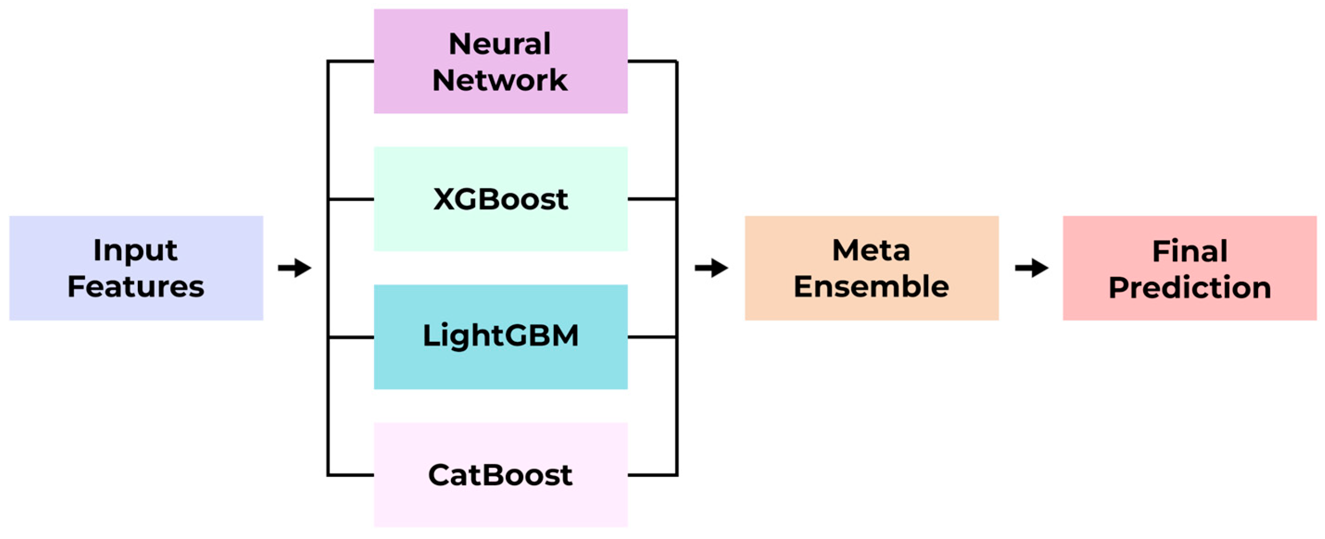
To develop a high-performance Meta Ensemble machine learning model capable of accurately estimating LTA discharge using a diverse set of globally distributed hydrological station metadata.

(2)

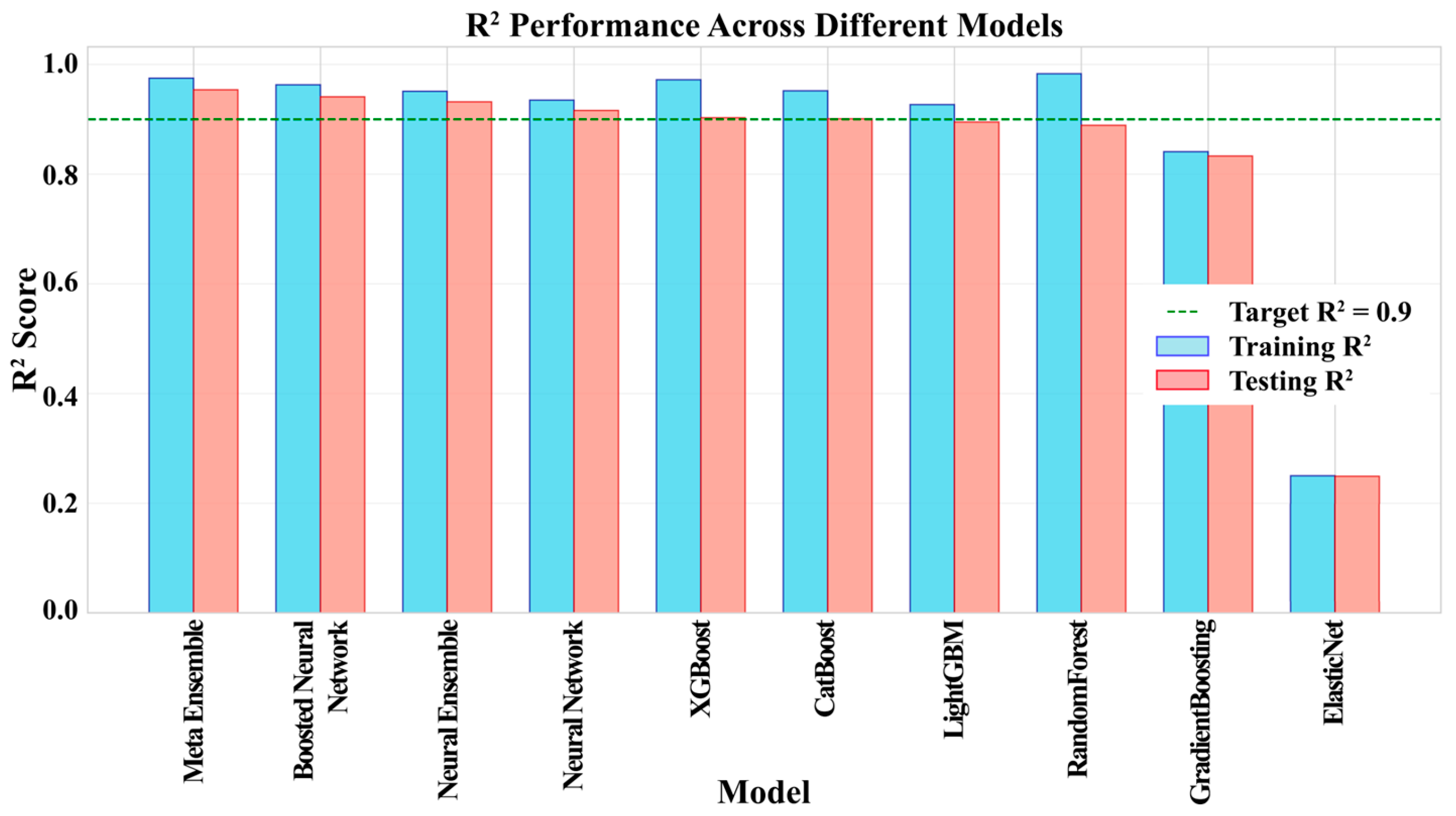
To systematically compare the performance of the proposed ensemble against various individual models, including a custom-designed neural network and several state-of-the-art gradient boosting machines.

(3)

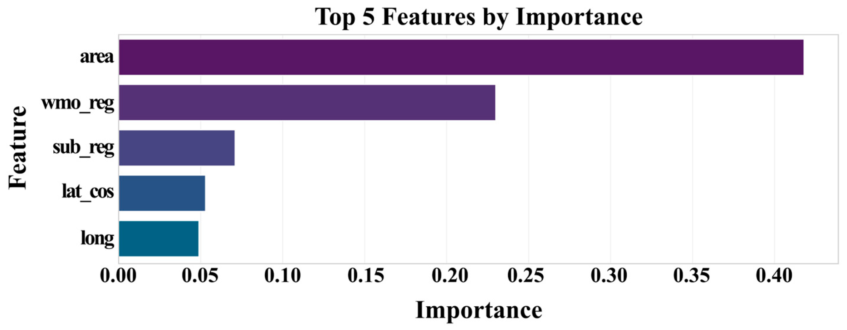
To identify and interpret the key geographical and physical catchment attributes that most significantly influence LTA discharge, using model-agnostic explanation techniques (SHAP).

(4)

To demonstrate the potential of this data-driven methodology as a scalable and cost-effective tool for large-scale water resource assessment, especially in ungauged or data-limited regions.

The remainder of this paper is structured as follows: Section 2 presents the materials and methods, detailing the data source, study area, data preprocessing, feature engineering, feature selection, and the development and evaluation framework for the predictive models. Section 3 discusses the results, providing an in-depth comparative analysis of the model performances, validation of the final model, and an interpretation of its predictions through SHAP analysis. Section 4 provides a discussion of the findings in the context of the existing literature and outlines the study’s limitations and future research directions. Finally, Section 5 concludes the study by summarizing the key findings and their implications.

2. Materials and Methods

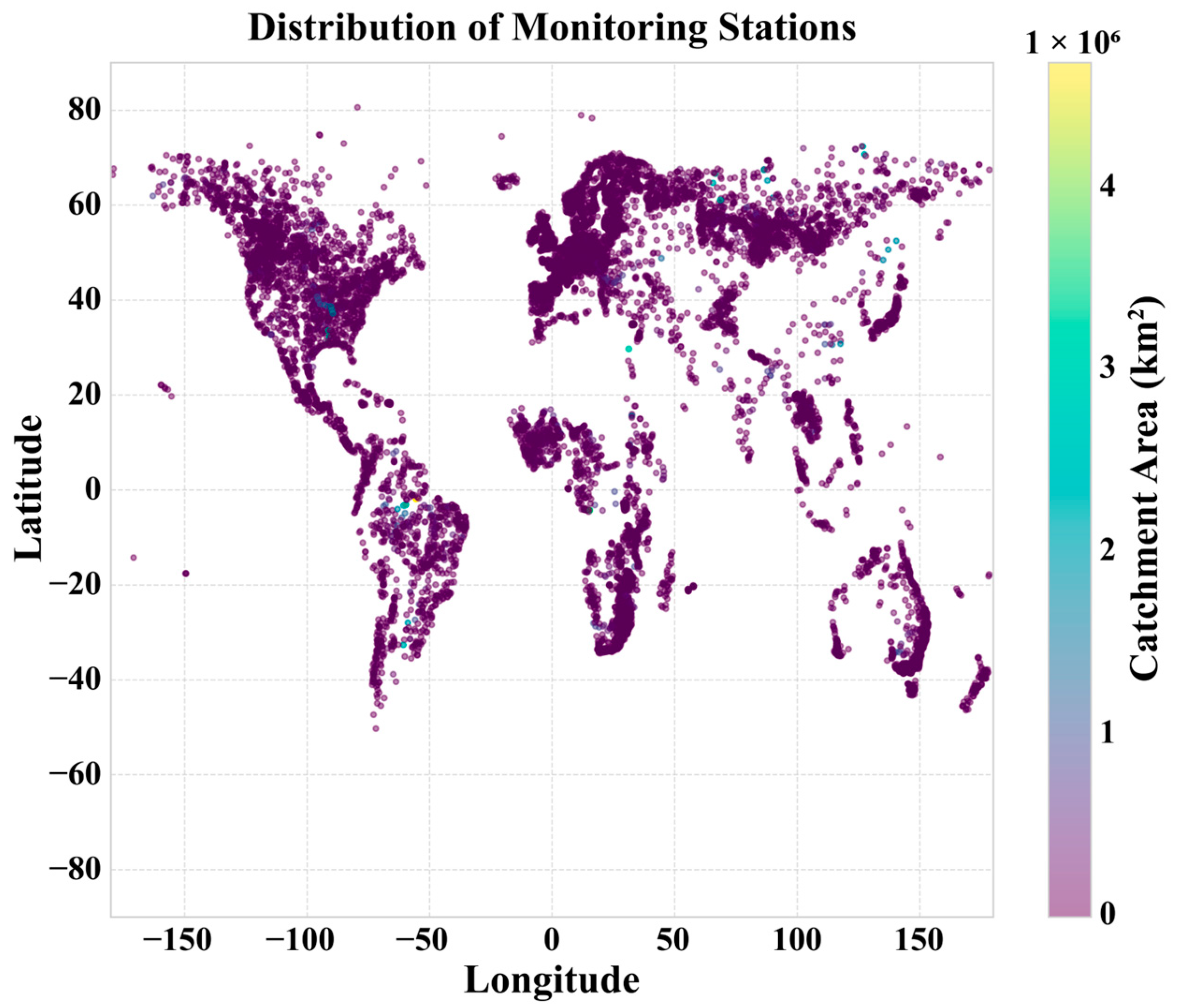
2.1. Data Source and Study Area

The analysis in this study is based on a global dataset of hydrological monitoring station metadata provided by the Global Runoff Data Centre (GRDC). The GRDC, operating under the auspices of the World Meteorological Organization (WMO), curates and disseminates data from river discharge stations worldwide, making its Station Catalogue an invaluable resource for large-scale hydrological research [60,61]. This comprehensive dataset allows for an analysis with a broad geographical scope, encompassing diverse climatic and hydrological regimes. The initial dataset contains 10,978 station records, each characterized by attributes such as geographical coordinates, catchment area, and key hydrological metrics.

The global distribution of these monitoring stations is visualized in Figure 1. A visual inspection reveals a significant concentration of stations in the Northern Hemisphere, particularly across North America and Europe, while coverage is sparser in regions such as Africa, South America, and Central Asia. This geographical bias is a known characteristic of global hydrological networks and presents a key challenge for global-scale modeling.

Further insight into spatial characteristics is provided by the station distributions along latitude and longitude (Figure 2). The latitudinal distribution histogram quantitatively confirms the bias towards the Northern Hemisphere, showing prominent peaks in the 40–60° N range (Figure 2a). The longitudinal distribution indicates major station clusters in the Americas (approximately −100° W to −70° W) and Europe (around 0° E to 30° E), with other notable concentrations in East Asia and Oceania (Figure 2b).

The distribution across the six World Meteorological Organization (WMO) regions is quantified in Figure 3. This chart clearly shows that Region 6 (Europe) and Region 4 (North America, Central America, and the Caribbean) host the largest numbers of stations. This is followed by Region 2 (Asia), while Regions 1 (Africa), 3 (South America), and 5 (South-West Pacific) have comparatively fewer stations, underscoring the regional disparities in monitoring network density.

The dataset’s utility extends to focused regional studies, even in areas often considered data-scarce. Figure 4 illustrates the geographical arrangement of monitoring stations across Eurasia, with particular attention to Central Asia, including Kazakhstan. In this visualization, station markers are scaled and colored according to their long-term average discharge, providing immediate insights into the hydrological variability of monitored rivers. This example highlights the dataset’s capacity for studying diverse hydrological regimes, including those in transboundary river basins like the Irtysh, which serves as a key area for hydrological research and water resource management [62].

2.2. Data Preprocessing and Feature Engineering

To prepare the raw GRDC metadata for machine learning modeling, a multi-step data preprocessing and feature engineering pipeline was implemented. The process began with data cleaning and type conversion. Key variables such as lta_discharge, r_volume_yr, and r_height_yr were initially stored as object types due to non-numeric entries like “-“. These were converted to a numeric format, and any records that could not be converted were treated as missing values (NaN). This initial step also addressed missing values present in other attributes, such as those related to monthly records.

A critical subsequent step was the transformation of the target variable. The primary target for this study is the Long-Term Average (LTA) discharge, defined as the arithmetic mean of daily discharge values over a multi-year observation period. As is common for hydrological data, the distribution of LTA values was highly right-skewed. To normalize this distribution, stabilize variance, and reduce the disproportionate influence of extreme outliers, a logarithmic transformation was applied using np.log1p(). All subsequent modeling was performed on this log-transformed target variable.

Following these initial steps, a comprehensive feature engineering process was undertaken to generate new, more informative predictors. This was crucial for enabling the models to capture complex non-linear relationships and interactions. Various transformations of the catchment area, including logarithmic, square root, and polynomial, were created to better represent its scaling effects. To handle the cyclical nature of geographical coordinates, sine and cosine transformations of latitude and longitude were computed, complemented by the calculation of the Haversine distance from the equator. To model combined effects, interaction terms between key predictors (e.g., area_wmo_interaction) and ratio features (e.g., area_to_altitude_ratio) were generated. Furthermore, temporal attributes such as station lifetime and operational age were calculated, alongside contextual features like the ratio of a station’s discharge to its regional average. Finally, to explicitly capture high-order interactions, second-degree polynomial features were generated for the top five most influential raw predictors.

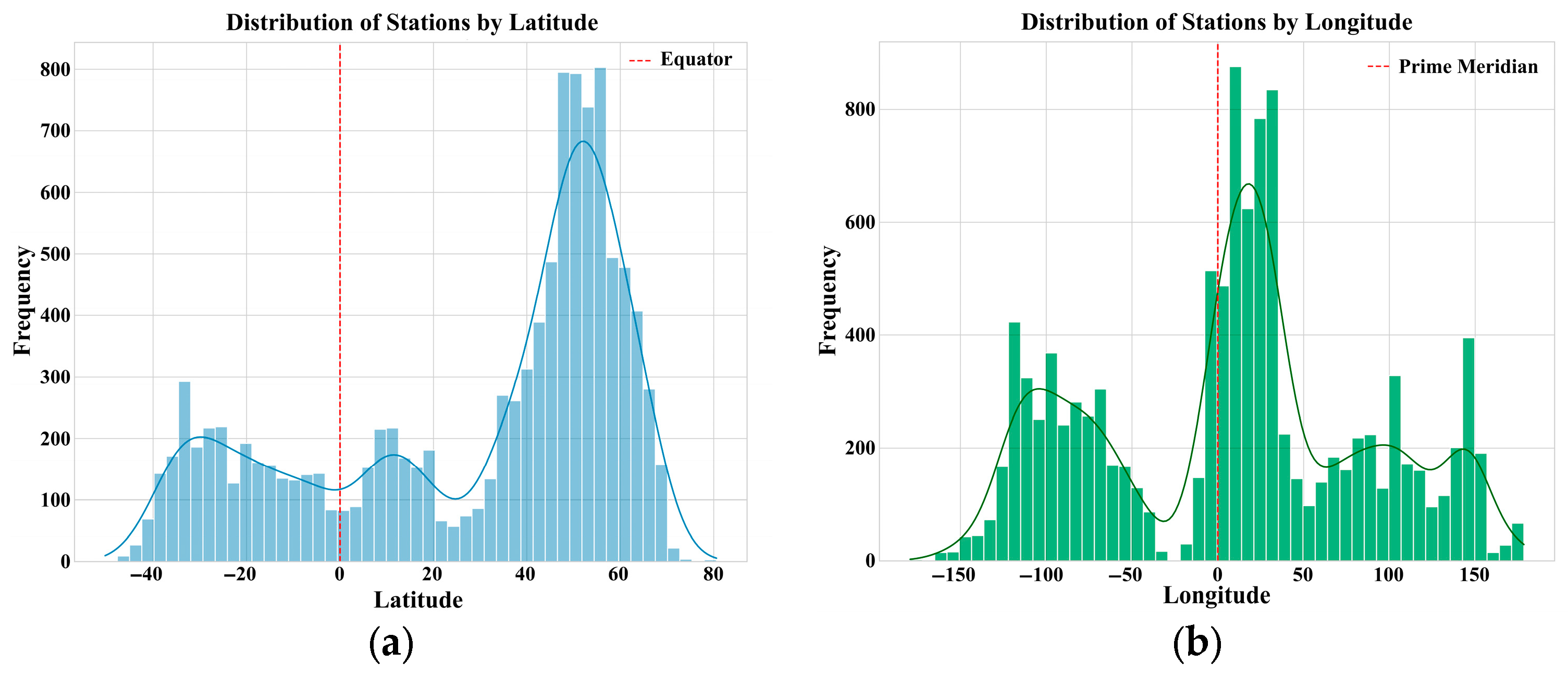
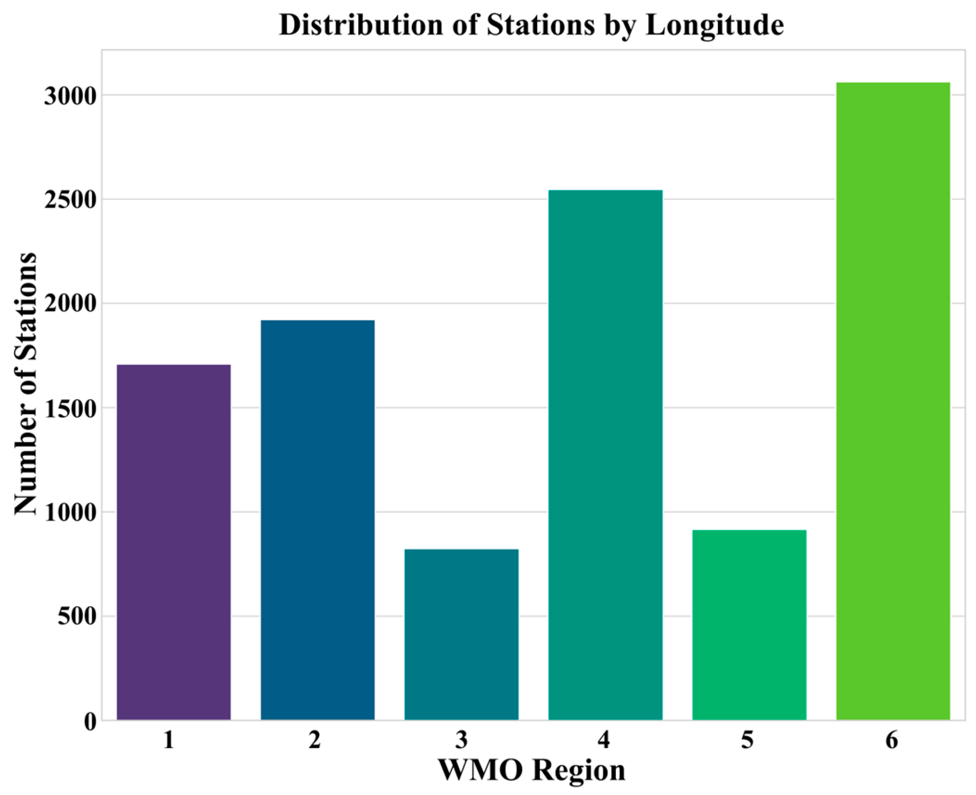
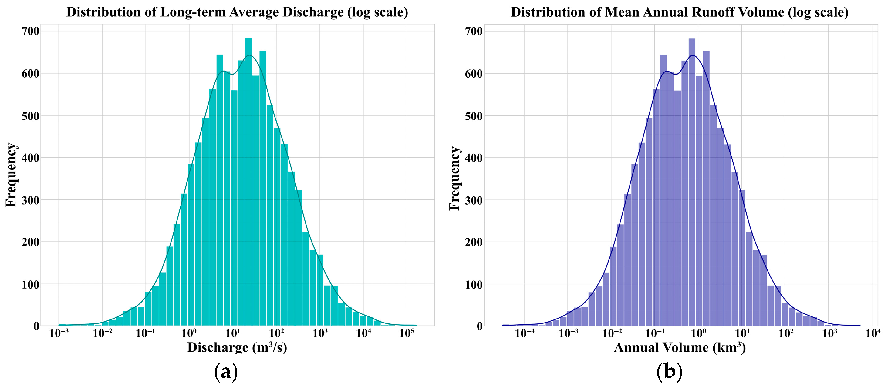
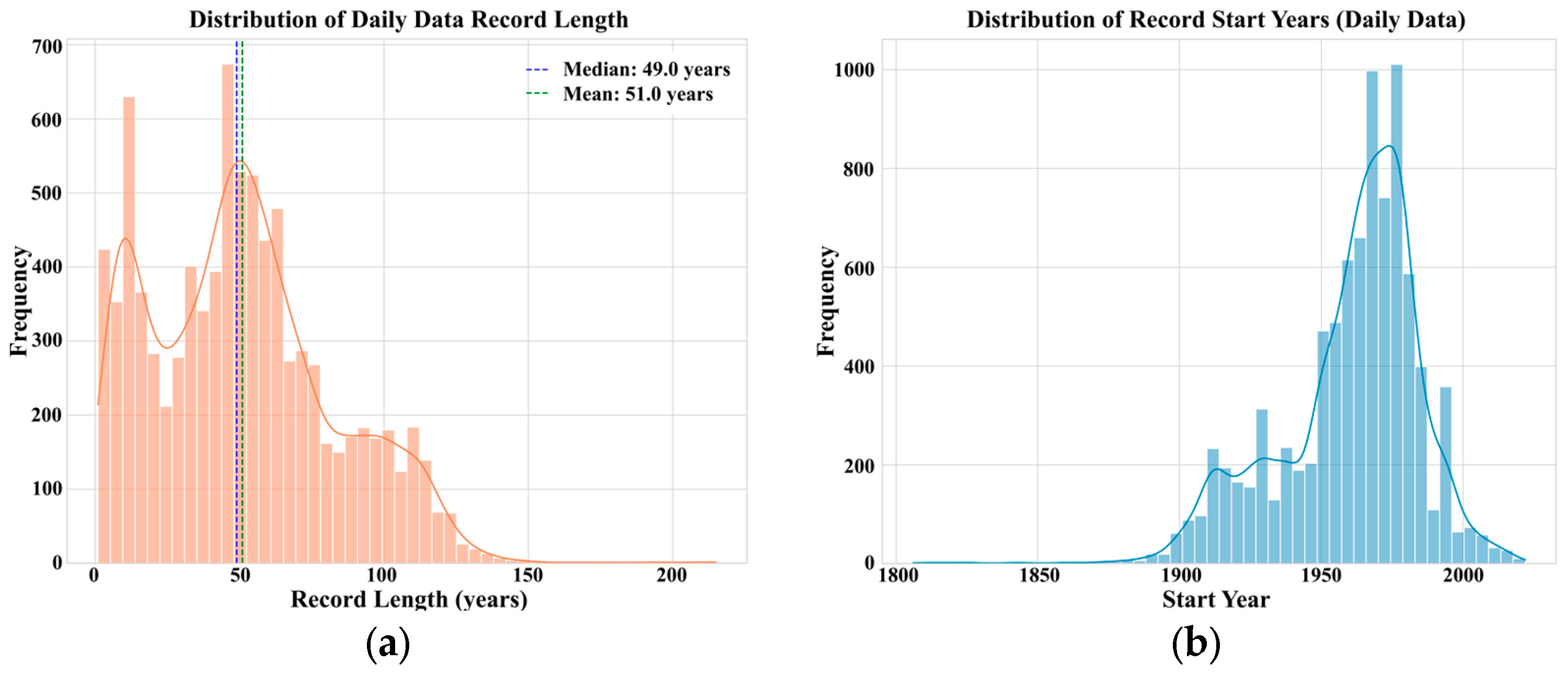
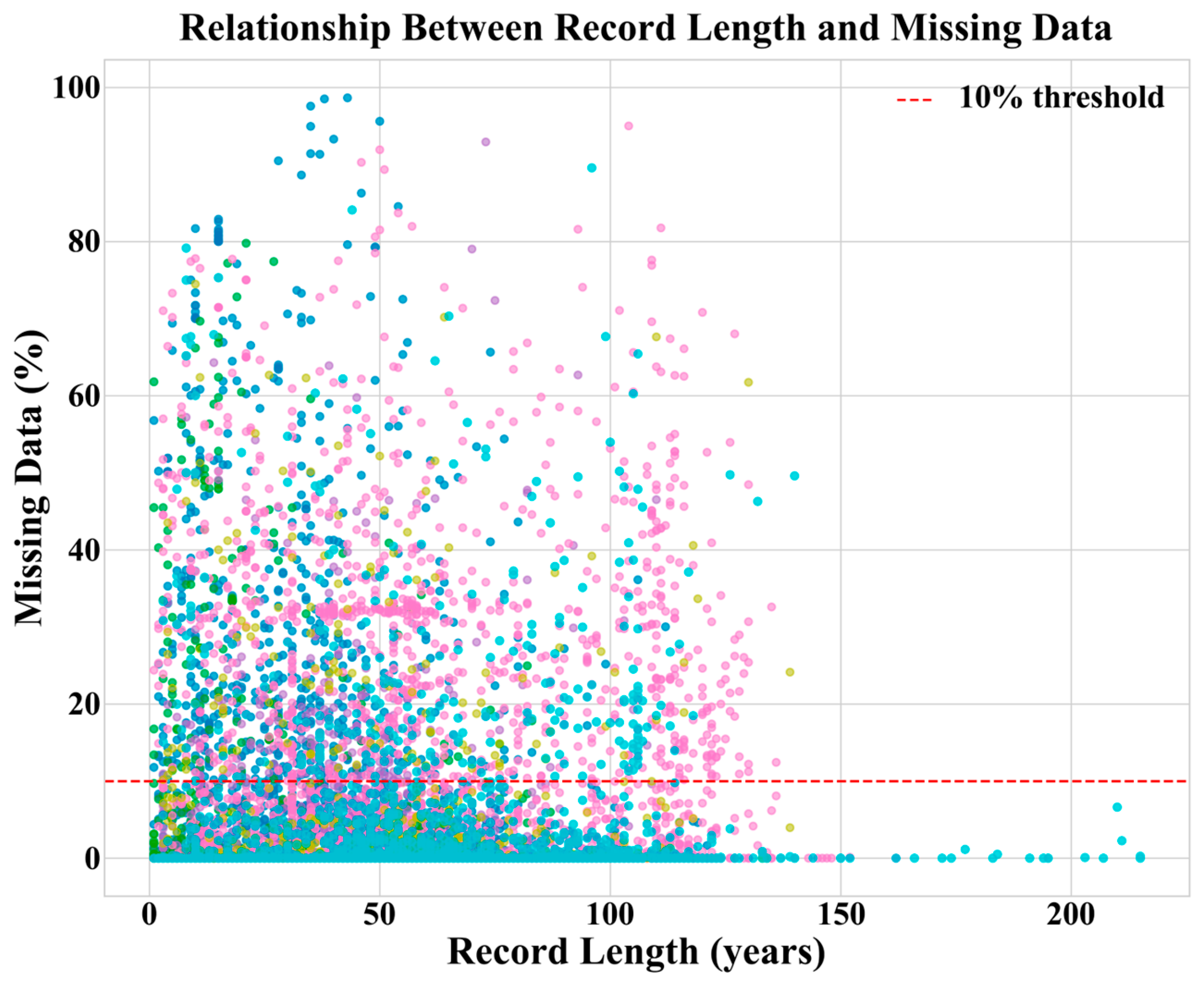
2.3. Exploratory Data Analysis and Data Quality

An exploratory data analysis (EDA) was conducted to understand the characteristics and quality of the GRDC dataset, which is crucial for informing model development.

The distributions of key hydrological variables were examined (Figure 5). As previously noted, the LTA discharge exhibits a strong positive skew, a typical feature in hydrology where a few large rivers dominate the dataset (Figure 5a). Similar right-skewed distributions were observed for mean annual runoff volume (Figure 5b).

An assessment of the daily data records provides insights into data quality (Figure 6). The distribution of record lengths shows a mean of approximately 51 years and a median of 49 years, indicating a substantial number of long-term observation series (Figure 6a). The distribution of record start years (Figure 6b) confirms that most monitoring began between 1950 and the late 1980s.

Further analysis of data quality reveals a complex interplay between the length of observation records and data completeness. As shown in Figure 7, while there is considerable scatter, many long-term records successfully maintain a low percentage of missing data, which is crucial for building robust models. A deeper, non-visualized analysis of the data further indicated that both the distribution of station quality and the median record lengths vary significantly across different WMO regions, with Europe (Region 6), for instance, demonstrating a higher concentration of long and complete observation series. This highlights the regional heterogeneity in data quality that the predictive models must account for.

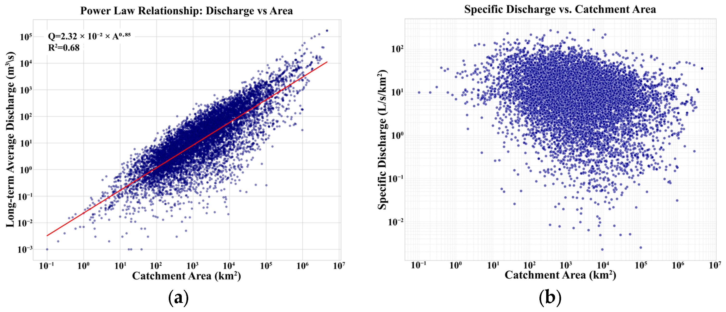
2.4. Feature Selection and Relationship Analysis

Following the EDA, a systematic analysis of variable relationships was performed, leading to a feature selection process designed to identify the most pertinent predictors for estimating LTA discharge. The primary goals were to enhance model performance, reduce multicollinearity, and improve interpretability.

The analysis began by examining the fundamental scaling relationships in the dataset (Figure 8). The relationship between catchment area and long-term average discharge, visualized on a log-log scale (Figure 8a), reveals a clear and strong power-law relationship approximated by Q ∝ A^0.85 (R² = 0.68). This confirms that the catchment area is a dominant physical driver of discharge and underscores the importance of using non-linear transformations of area (such as area_log) as a primary predictive feature.

To further investigate these scale effects, the relationship between specific discharge (discharge per unit area) and catchment area was also analyzed (Figure 8b). Unlike the strong trend in the first plot, this visualization shows considerable scatter without a universal pattern. This suggests that while catchment size is a primary driver, the efficiency of runoff generation is highly variable and influenced by a complex interplay of other regional factors, such as climate and topography, which the model must learn from other features.

To identify geographical groupings of stations with potentially similar hydrological characteristics, K-Means clustering was applied to the station metadata. The Elbow method [63,64] was used to determine an appropriate number of clusters, suggesting an optimum (k) around 4 or 5, where the rate of decrease in the sum of squared distances diminishes (Figure 9).

The resulting spatial distribution for k = 5 is visualized in Figure 10. The map reveals distinct geographical clusters that largely correspond to continental regions (e.g., North America, Europe, South America). This indicates the presence of strong spatial patterns in the dataset, which can be effectively leveraged by the models, particularly through features like geographical coordinates and regional identifiers (e.g., wmo_reg).

The final feature selection process was guided by two primary methods: correlation analysis and model-based feature importance. A Pearson correlation analysis identified features with the strongest linear relationship to the log-transformed target variable. As expected, engineered features derived from area and runoff volume (area_log, r_volume_yr_log) showed the highest correlations. A heatmap of the top 15 correlated features is presented in Figure 11, which also helps to identify potential multicollinearity among some of the top predictors. To further explore these interdependencies, hierarchical clustering was applied to the variables, confirming that area, lta_discharge, and r_volume_yr are closely related (Figure 12).

To complement this analysis, feature importance was assessed using a preliminary XGBoost model. This model-based approach ranks features based on their contribution to reducing prediction error. The results, shown in Figure 13, unequivocally identified area as the most important feature, followed by regional identifiers (wmo_reg, sub_reg) and geographical coordinates (lat_cos, long). Based on a synthesis of these analyses—prioritizing features with high correlation to the target, high model-based importance, and including key engineered features to capture non-linearities—a final set of 33 features was selected for the predictive modeling phase. The final feature set is detailed in

Table 1. Final set of 33 selected features for predictive modeling, categorized by type.

Category	Feature Name	Description	Data Type
Raw Identifiers & Regional	grdc_no	Unique GRDC station identifier	int64
	wmo_reg	WMO region code	int64
	sub_reg	WMO subregion code	int64
Raw Geographic & Topographic	lat	Latitude	float64
	lon	Longitude	float64
	altitude	Altitude of gauge zero	float64
Raw Catchment	area	Catchment area	float64
Engineered Catchment	area_log	Log-transformed catchment area (log1p)	float64
	area_sqrt	Square root of catchment area	float64
Engineered Geographic	lat_sin	Sine of latitude (radians)	float64
	lat_cos	Cosine of latitude (radians)	float64
	long_sin	Sine of longitude (radians)	float64
	long_cos	Cosine of longitude (radians)	float64
	distance_from_equator	Haversine distance from the equator (km)	float64
Engineered Ratio	area_to_altitude_ratio	Ratio of area to (altitude + 1)	float64
Engineered Interaction	lat_long_interaction	Product of latitude and longitude	float64
	area_wmo_interaction	Product of area and WMO region code	float64
Engineered Temporal	station_lifetime	Duration of station operation (t_end–t_start)	int64
Engineered Regional Context	discharge_to_region_mean	Station LTA discharge relative to WMO region mean discharge	object
	discharge_to_region_median	Station LTA discharge relative to WMO region median discharge	object
Engineered Polynomial (Degree 2)	poly_0, …, poly_14	Interaction term from top 5 raw features (e.g., area × wmo_reg)	float64

.

2.5. Predictive Model Development

The core of this study is a hybrid modeling strategy that leverages the strengths of multiple machine learning paradigms to maximize predictive accuracy. This involved developing several diverse individual models, which were then combined within a final meta-ensemble framework.

A variety of model architectures were developed to capture different types of patterns within the data. A custom Advanced Neural Network (NN) was designed using the TensorFlow/Keras framework. Recognizing the paramount importance of the catchment area, the NN architecture features a specialized, separate processing path for the area feature, allowing the model to learn its influence directly. This path is then concatenated with the main network path, which consists of multiple hidden layers with residual connections, inspired by ResNet architectures [65], to facilitate the training of a deep network. The complete architecture is visualized in Figure 14. In addition to the neural network, a suite of Gradient Boosting Machines (GBMs) was trained, including XGBoost [66], LightGBM [67], and CatBoost [68]. These tree-based ensemble algorithms were selected for their state-of-the-art performance on tabular data and their ability to capture complex non-linear interactions, providing a robust alternative modeling approach to the NN.

To ensure each model reached its full potential, hyperparameters were systematically tuned using the Optuna framework, which employs Bayesian optimization techniques. This approach efficiently explores the complex hyperparameter space to find optimal configurations for learning rates, network depth, and regularization terms, among others. This rigorous optimization was crucial for maximizing the performance of each base learner before ensembling.

The cornerstone of the predictive strategy is a Meta-Ensemble Model, conceptually illustrated in Figure 15. This final model aggregates the predictions from the best-performing individual models (the optimized NN, XGBoost, LightGBM, and CatBoost). Instead of a simple average, it uses a weighted combination where the weights are themselves optimized on a validation set to maximize the final R² score. This strategy allows the final model to capitalize on the unique strengths and perspectives of each base model, often leading to performance superior to any single constituent.

2.6. Data Preparation for Modeling and Validation Strategy

The final step in the data preparation pipeline involved cleaning, partitioning, and scaling the data. First, a final cleaning was performed by applying a listwise deletion to the dataset, removing any rows that contained missing values in either the 33 selected features or the target variable. This process yielded a final, clean dataset of 10,586 samples, retaining 96.43% of the original station records.

This clean dataset was then partitioned into training (80%) and testing (20%) subsets. This split resulted in 8468 samples for training the models and 2118 samples reserved for the final, independent evaluation. A fixed random state (SEED = 42) was used during partitioning to ensure the reproducibility of the results.

Finally, feature scaling was applied to standardize the numerical features. The RobustScaler method from Scikit-learn was chosen for this task. This scaler is particularly effective for datasets containing outliers, as it scales data based on the interquartile range, making it robust to extreme values. Crucially, the scaler was fitted only on the training data and then used to transform both the training and testing sets. This strict separation prevents any data leakage from the test set into the training process, ensuring an unbiased and valid evaluation of the models’ generalization performance.

2.7. Evaluation and Interpretation Methods

The performance of all predictive models was rigorously evaluated using a set of standard statistical metrics. The Coefficient of Determination (R²) was used to measure the proportion of variance in the target variable explained by the model. The Root Mean Squared Error (RMSE) was calculated to assess the magnitude of prediction errors on the log-transformed scale. Additionally, the Mean Absolute Error (MAE) was computed on both the log-transformed scale and, crucially, on the original discharge units (m³/s) by back-transforming the predictions. This provides a direct, physically interpretable measure of the model’s average error. The mathematical formulas for these metrics are provided in Equations (1)–(3).

The Coefficient of Determination (R²) was used to quantify the proportion of variance in the log-transformed discharge that the model could explain. This metric is mathematically expressed as follows:

$$R^2=1-{\displaystyle \frac{\sum _{i=1}^n{(y_i-{\widehat{y}}_i)}^2}{\sum _{i=1}^n{(y_i-\overline{y})}^2}}$$

(1)

where $y_i$ represents the observed log-transformed discharge value for the i-th sample, ${\widehat{y}}_i$ represents the predicted log-transformed discharge value for the i-th sample, $\overline{y}$ represents the mean of all observed log-transformed discharge values, and n represents the total number of samples in the dataset.

Root Mean Squared Error (RMSE) provided a measure of the typical magnitude of the prediction errors on the log scale. RMSE is calculated as follows:

$$RMSE=\sqrt{{\displaystyle \frac{1}{n}}{\sum }_{i=1}^n{(y_i-{\widehat{y}}_i)}^2},$$

(2)

where $y_i$ represents the observed log-transformed discharge value for the i-th sample, ${\widehat{y}}_i$ represents the predicted log-transformed discharge value for the i-th sample, and n represents the total number of samples in the dataset.

Mean Absolute Error (MAE) offered an alternative measure of average error magnitude, less sensitive to outliers than RMSE. MAE is calculated as follows:

$$MAE={\displaystyle \frac{1}{n}}{\sum }_{i=1}^n\left|y_i-{\widehat{y}}_i\right|,$$

(3)

where $y_i$ represents the observed log-transformed discharge value for the i-th sample, ${\widehat{y}}_i$ represents the predicted log-transformed discharge value for the i-th sample, n represents the total number of samples in the dataset, and ∣⋅∣ denotes the absolute value function.

To address the inherent “black-box” nature of complex ensemble models and to understand why the model makes certain predictions, we employed SHAP [51,52]. SHAP is a game-theoretic approach to explain the output of any machine learning model. It connects optimal credit allocation with local explanations using the classic Shapley values from game theory. For each prediction, SHAP assigns each feature an importance value—the SHAP value—representing the magnitude and direction of its contribution to moving the prediction away from the baseline (average) prediction. This allows for a detailed analysis of feature influence on both an individual and global level. In this study, SHAP was used to do the following: (1) Generate global feature importance plots. These plots rank features based on the mean absolute SHAP value across all samples, providing a clear overview of which factors have the most significant overall impact on LTA discharge estimation; (2) Create feature dependence plots. These plots visualize how the value of a single feature affects its SHAP value (i.e., its impact on the prediction), often revealing complex non-linear relationships and interaction effects with other features. The visual results of this analysis, including SHAP summary and dependence plots, are presented in Section 3.

3. Results

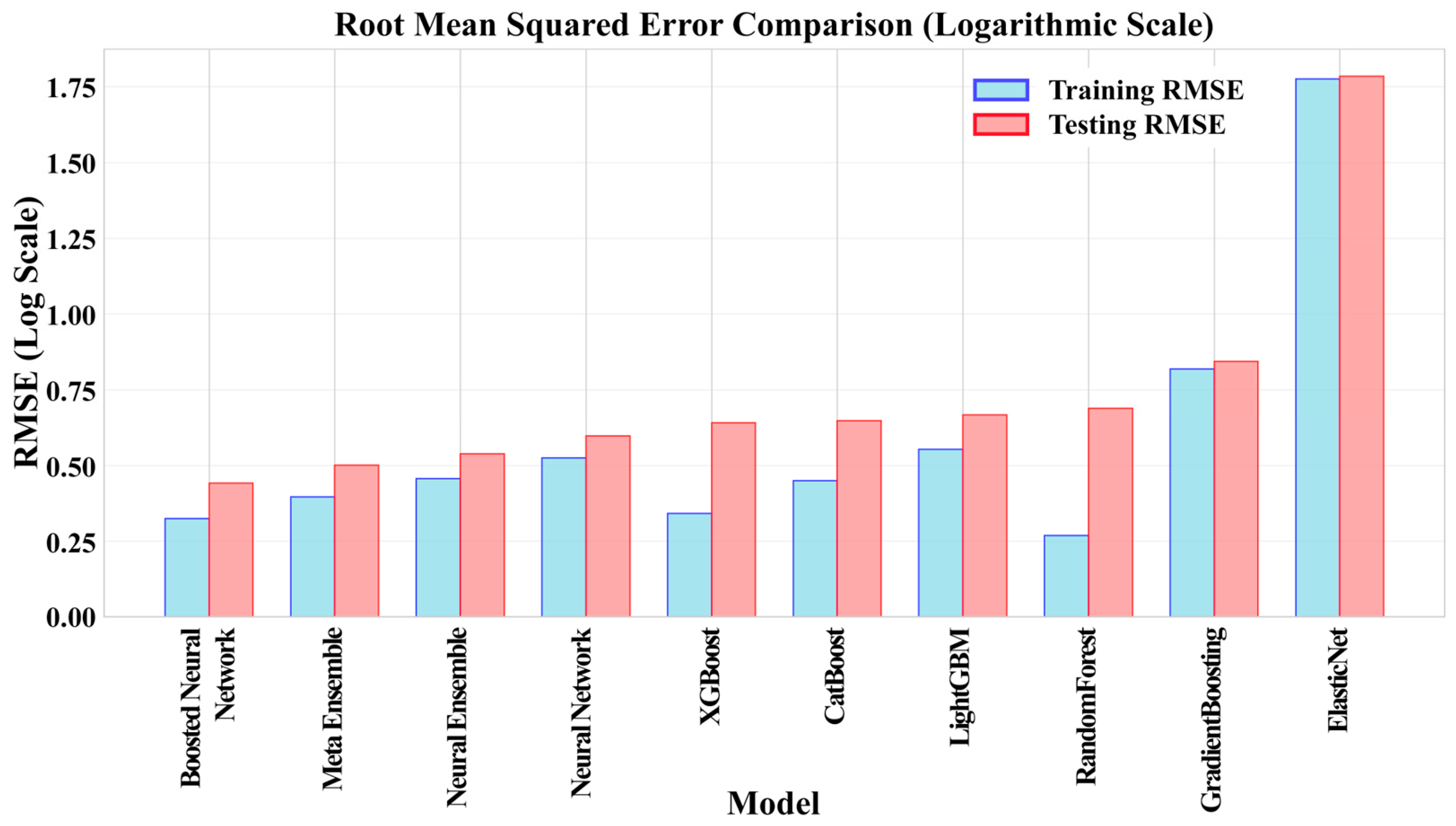
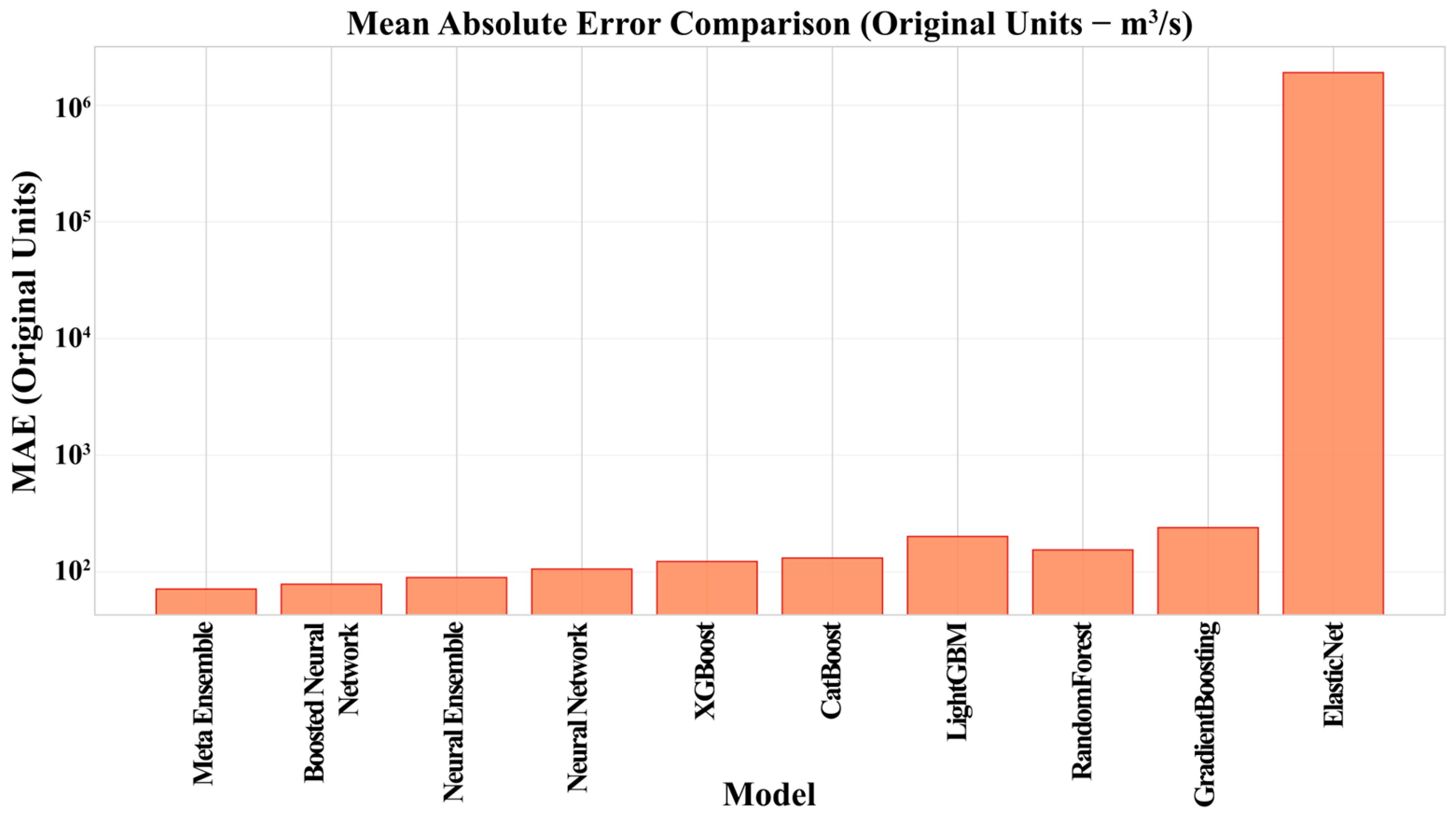
3.1. Comparative Model Performance

A comprehensive evaluation was conducted to compare the predictive performance of all developed models, from simple baselines to advanced ensembles. The key performance metrics—Coefficient of Determination (R²), Root Mean Squared Error (RMSE) on the logarithmic scale, and Mean Absolute Error (MAE) on the original discharge scale (m³/s)—were calculated for both the training and testing datasets to assess accuracy and generalization capability.

The performance metrics for all evaluated models are summarized in

Table 2. Performance metrics of all evaluated models on the training and testing sets.

Model	Train_R2	Test_R2	Train_RMSE	Test_RMSE	Train_MAE	Test_MAE
ElasticNet	0.25	0.249	1.776	1.785	449,598.39	1,904,236.58
RandomForest	0.983	0.889	0.268	0.688	75.35	154.61
GradientBoosting	0.841	0.833	0.818	0.843	173.55	239.62
XGBoost	0.972	0.903	0.341	0.641	70.25	122.9
LightGBM	0.72	0.895	0.553	0.667	129.61	201.36
CatBoost	0.952	0.901	0.449	0.648	95.67	131.45
Neural Network	0.935	0.916	0.524	0.597	83.21	105.82
Neural Ensemble	0.951	0.932	0.456	0.538	70.46	89.73
Boosted Neural Network	0.963	0.941	0.396	0.501	65.78	78.41
Meta Ensemble	0.975	0.954	0.324	0.442	62.13	71.28

. A clear performance hierarchy emerged. The baseline linear model (ElasticNet) demonstrated poor performance (Test R² ≈ 0.25), indicating its inability to capture the complex non-linear relationships in the data. Traditional ensemble methods like RandomForest and GradientBoosting showed considerable improvement but were ultimately surpassed by the more advanced algorithms.

The individual advanced models, including the custom Neural Network (Test R² = 0.916) and the GBMs (XGBoost, CatBoost, LightGBM, Test R² ≈ 0.90), performed strongly. However, the highest performance was consistently achieved by the ensemble strategies. The Neural Ensemble and the Boosted Neural Network reached Test R² values of 0.932 and 0.941, respectively. Ultimately, the Meta Ensemble model, which combines predictions from the top-performing models with optimized weights, yielded the best results, achieving a Test R² of 0.954 on the independent test set.

The comparative R² scores are visually summarized in Figure 16. This chart clearly illustrates that all advanced models, and particularly the ensemble methods, successfully met and exceeded the predefined performance target of R² = 0.9. The small gap between training (blue) and testing (light red) scores for the top models, especially the Meta Ensemble, indicates good generalization and a low risk of overfitting.

The error metrics provide further evidence of the Meta Ensemble’s superiority. Figure 17 shows the RMSE on the logarithmic scale, where the Meta Ensemble achieved the lowest test error (0.442), indicating the highest accuracy on the transformed scale.

More importantly, when evaluating the error in the original physical units, the practical advantage of the advanced models becomes evident. Figure 18 plots the Mean Absolute Error (MAE) in m³/s on a logarithmic axis to accommodate the vast range of error magnitudes. The Meta Ensemble model achieved the lowest practical error with a Test MAE of 71.3 m³/s, a significant improvement over other models and a highly accurate result in the context of large-scale hydrological estimation.

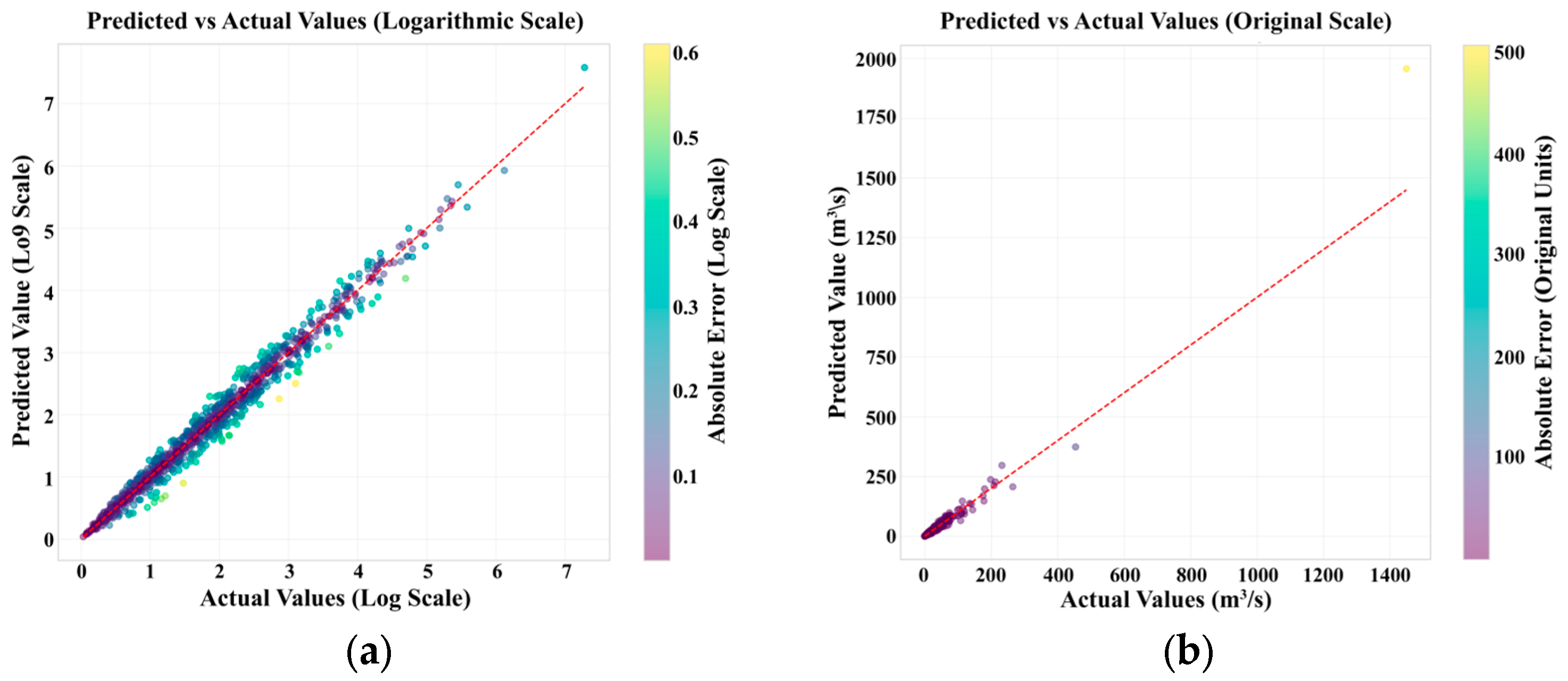
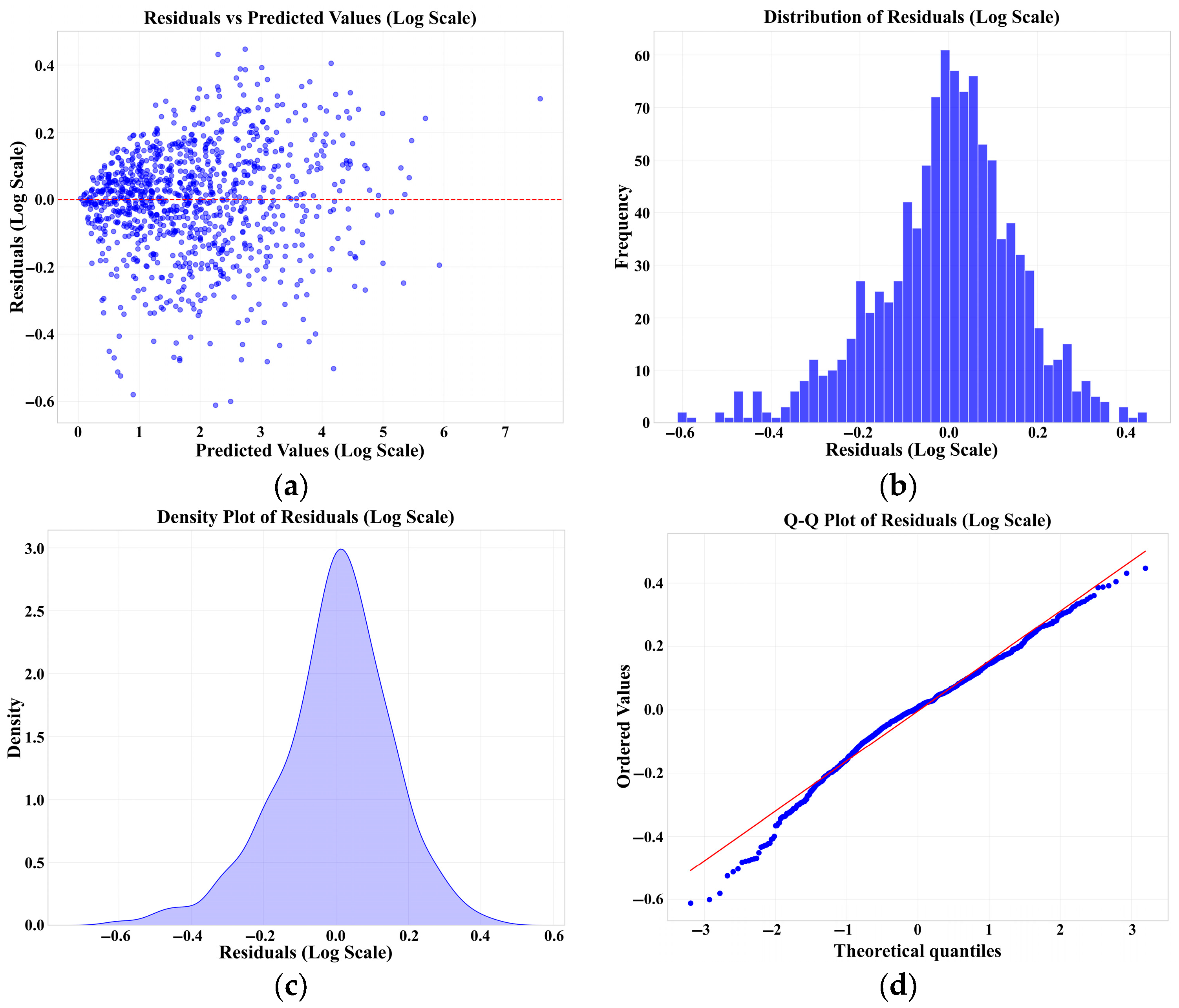
3.2. Final Model Performance and Validation

A detailed validation of the final Meta Ensemble model was performed to assess its accuracy and identify any potential systematic biases. This involved analyzing the relationship between predicted and actual values on both logarithmic and original scales, and conducting a thorough residual analysis.

Figure 19 presents scatter plots of the model’s predicted versus actual discharge values for the independent test set. On the logarithmic scale (Figure 19a), the data points cluster tightly around the 1:1 line (dashed red line), indicating a very strong correlation and high agreement across several orders of magnitude. The high R² value of 0.954 quantitatively confirms this excellent fit.

To provide a more intuitive understanding of the model’s performance in physically meaningful units, the same comparison is shown on the original discharge scale (m³/s) in Figure 19b. This plot again confirms the model’s high accuracy, with most points closely following the 1-to-1 line. While some larger errors are visible for very high discharge values, which is a common challenge in hydrological modeling, the model maintains a strong predictive capability across the full range of observed flows. The color of each point in both plots represents the absolute prediction error, visually confirming that the vast majority of predictions have a low error (darker points).

A comprehensive residual analysis was conducted to ensure the model’s predictions are unbiased (Figure 20). The plot of residuals vs. predicted values (Figure 20a) shows that the residuals are randomly scattered around the horizontal zero line, with no obvious non-linear patterns. This suggests that the model has successfully captured the underlying relationships in the data. The distribution of residuals (Figure 20b), visualized as a histogram, and the corresponding density plot (Figure 20c) demonstrate that the errors are approximately normally distributed and centered close to zero, which is a desirable characteristic of a well-calibrated model. Finally, the Quantile-Quantile (Q-Q) plot of residuals (Figure 20d) compares the quantiles of the residuals against the theoretical quantiles of a standard normal distribution. The points fall closely along the diagonal line, further confirming the normality of the errors, with only minor deviations at the tails, which correspond to the occasional larger errors seen in the scatter plots.

Collectively, these diagnostic plots validate the Meta Ensemble model, demonstrating that it provides accurate and largely unbiased predictions. The errors are randomly distributed and approximately normal, confirming the model’s robustness and suitability for its intended application.

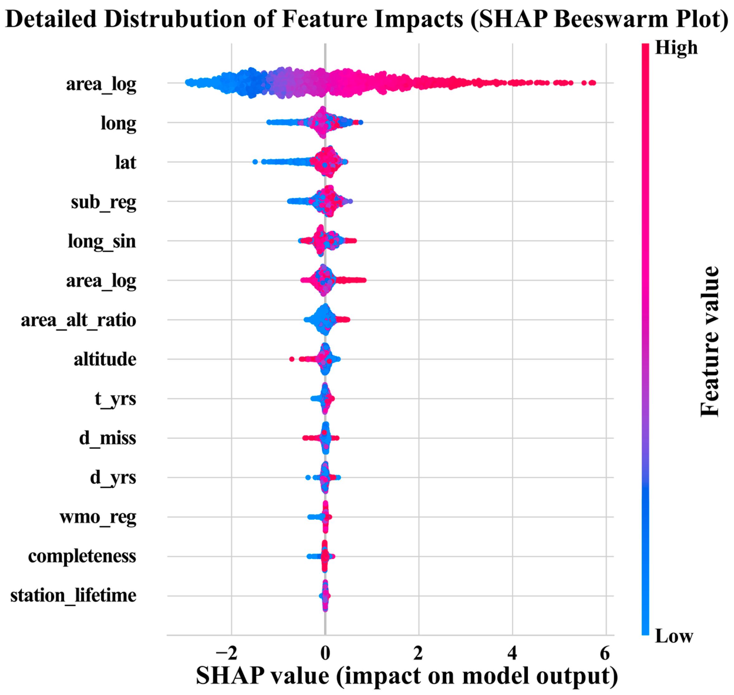
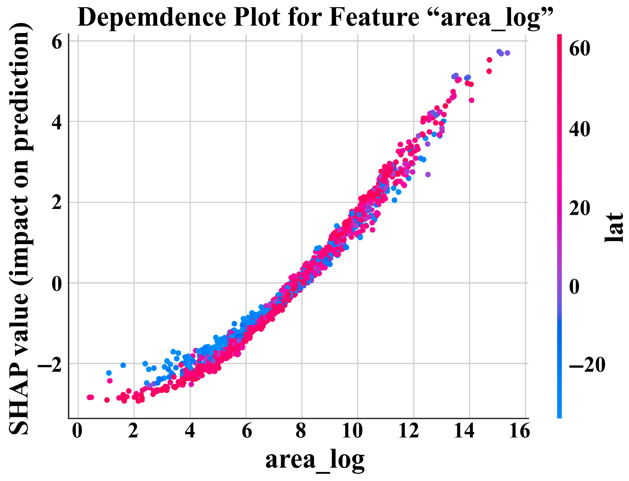
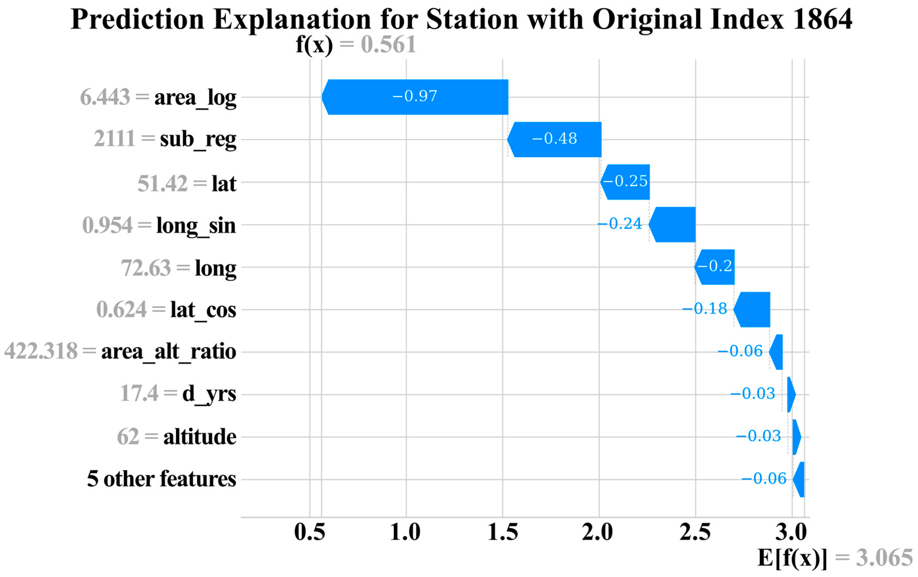
3.3. Model Interpretation and Feature Importance Using SHAP

To move beyond performance metrics and understand why the Meta Ensemble model is successful, we employed the SHAP framework for model interpretation. This analysis provides crucial insights into the model’s inner workings, revealing the most influential features and the nature of their impact on LTA discharge predictions.

The global importance of each feature is summarized in the SHAP summary plot (Figure 21), which ranks features by their mean absolute SHAP value across all test samples. The results unequivocally confirm that log-transformed catchment area (area_log) is the single most dominant predictor of LTA discharge, having a significantly larger impact than any other feature. This aligns with fundamental hydrological principles. Following area_log, geographical location features—long (longitude) and lat (latitude)—and regional identifiers (sub_reg) are the next most important predictors. This highlights the model’s ability to learn complex spatial patterns of water availability. Other engineered features like area_alt_ratio and temporal characteristics (t_yrs) also make meaningful contributions, justifying the feature engineering efforts.

While the summary plot shows global importance, SHAP dependence plots reveal how a feature’s value affects the prediction. The dependence plot for area_log (Figure 22) shows a strong, near-linear positive relationship: as the log of the catchment area increases, so does its positive impact on the predicted LTA discharge. This is physically intuitive, as larger catchments are expected to generate more runoff. The color interaction with lat (latitude) suggests a secondary effect, where for a given catchment size, stations at higher latitudes (red points) tend to have a slightly different response, which the model has successfully captured.

The SHAP analysis provides strong evidence that the Meta Ensemble model’s success is not arbitrary but is based on learning hydrologically meaningful relationships from the data. The model correctly identifies the primary physical driver (catchment area) and effectively uses geographical and regional context to refine its predictions. This interpretability builds confidence in the model’s reliability and its potential for practical application in hydrological assessment. We can also analyze the prediction for a single station. For example, a waterfall plot (Figure 23) for a specific station shows how each feature contributes to pushing the prediction from the base value (the average prediction over the dataset) to the final output. This local-level explanation is invaluable for diagnosing model behavior on individual cases.

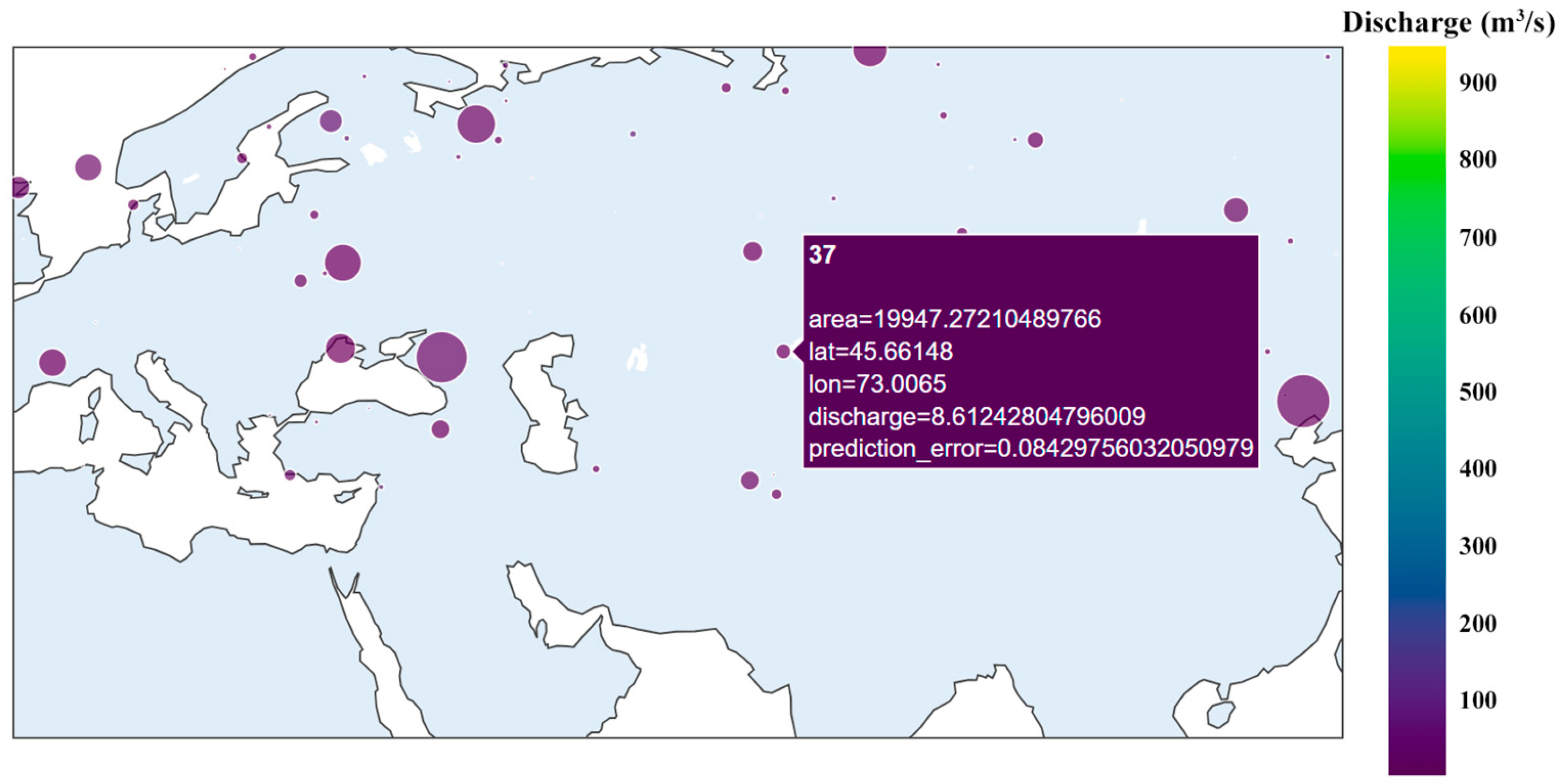
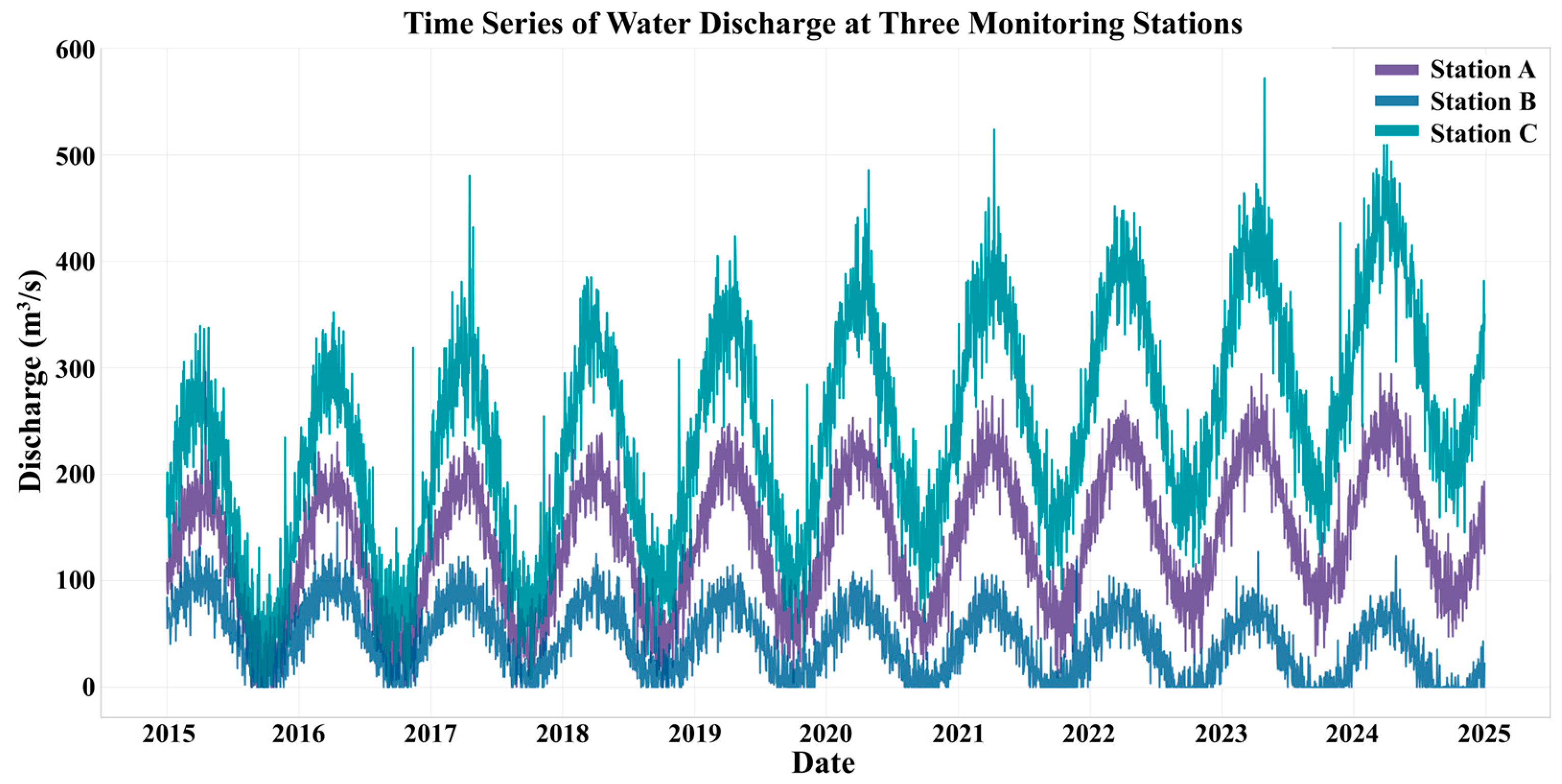
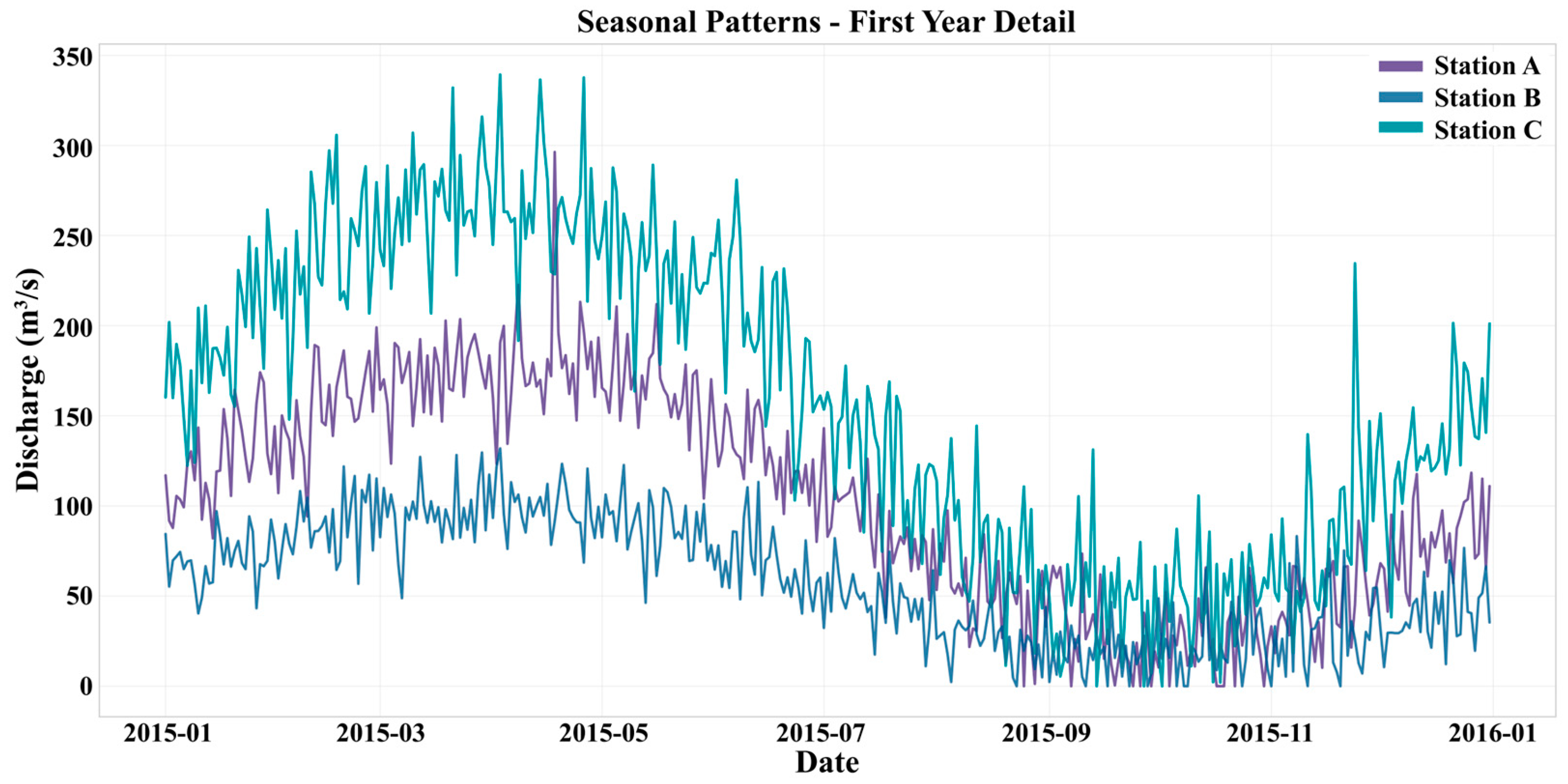
3.4. Example of Time Series Visualization

To illustrate how the outputs of hydrological analysis can be presented for practical interpretation, this section provides an example of time series visualization. Effective communication of results is crucial for supporting decision-making in water resource management.

Figure 24 presents a plot of synthetically generated daily discharge data for three hypothetical monitoring stations (A, B, and C) over a ten-year period. It is important to clarify that these are not direct outputs of the LTA prediction model but rather illustrative examples of the type of time-series data that our framework is designed to analyze and that can be visualized in a potential monitoring dashboard. This multi-year overview clearly displays distinct seasonal patterns, which are characteristic of many river systems, as well as significant differences in flow magnitude between the stations. For instance, Station C consistently exhibits higher peak flows compared to Stations A and B. Such a visualization effectively captures inter-annual variability, allowing for the identification of particularly wet or dry years and providing a long-term context for detecting anomalies.

Figure 25 provides a more detailed view of the first year (2015) of the same record. This zoomed-in perspective allows for closer inspection of the seasonal hydrograph shape and short-term variability. It reveals important characteristics such as the timing of high-flow events, the shape of recession curves, and baseflow conditions during dry periods. Such views are essential for operational analysis, enabling stakeholders to assess specific hydrological processes and rainfall–runoff dynamics.

The dual-scale visualization approach demonstrates how hydrological data can be effectively presented to support both long-term strategic planning and short-term operational analysis, bridging the gap between raw data and actionable insights for water resource management.

4. Discussion

4.1. Interpretation of Model Performance and Feature Importance

This study introduced and validated an advanced ensemble machine learning framework for estimating long-term average (LTA) discharge from global hydrological station metadata. The high predictive accuracy achieved by the Meta Ensemble model (Test R² = 0.954) demonstrates the significant potential of data-driven approaches for large-scale water resource assessment.

The superior performance of the Meta Ensemble model over individual learners, including a sophisticated custom Neural Network and state-of-the-art GBMs, aligns with a well-established consensus in machine learning: ensemble methods tend to be more robust and accurate by averaging out the biases of individual models [51,62,69]. The diversity of the base learners (neural network and tree-based models) likely allowed the ensemble to capture different facets of the complex, non-linear relationships between station metadata and LTA discharge.

The model interpretability analysis using SHAP provides crucial validation of the model’s logic. The overwhelming importance of catchment area (area and its transformations) as the primary predictor is consistent with fundamental hydrological principles, confirming that the model has learned a physically plausible relationship. The significant contribution of geographical coordinates (lat, long) and regional identifiers (wmo_reg, sub_reg) highlights the model’s ability to effectively learn and apply spatial context, essentially performing a form of implicit regionalization to account for climatic and geological variability not explicitly included as features. This capacity to learn from spatial context is a key strength of applying ML to large, geographically diverse datasets.

4.2. Comparison with Existing Research

While a vast body of literature exists on applying machine learning to hydrology, most studies focus on dynamic streamflow forecasting using time-series data as inputs [36,46,62,69]. Our work addresses a different but equally important problem: estimating a static, long-term characteristic (LTA) from metadata. This task is more aligned with regionalization studies and methods for prediction in ungauged basins (PUB), where the goal is to transfer information from gauged to ungauged locations based on their physical characteristics [12,37]. Compared to traditional regression-based regionalization methods, our ensemble ML approach offers a more flexible and powerful framework for capturing complex, non-linear relationships on a global scale. Unlike systems focused purely on real-time data from IoT sensors [8,29,32], our approach leverages historical, aggregated information embedded in the GRDC catalogue, making it suitable for strategic planning and large-scale assessment rather than operational forecasting.

4.3. Practical Implications and Potential for Operationalization

The developed model has significant practical implications. It provides a robust, cost-effective tool for estimating baseline water availability in regions with sparse or non-existent gauging networks. This can be invaluable for preliminary water resource planning, climate change impact assessment, and the initial design of hydraulic structures. For example, for a proposed dam or irrigation project in a data-scarce region like Central Asia, the model can provide a rapid first-order estimate of LTA discharge, requiring only basic geographical and catchment information.

While this study focused on developing the predictive model, its outputs could be integrated into a broader, operational monitoring system. A conceptual architecture for such a system is presented in Figure 26. In such a system, our LTA estimation model could serve two roles: (1) providing baseline “normal” discharge values against which real-time data from IoT sensors can be compared for anomaly detection, and (2) generating virtual time series or filling gaps in records for other hydrological models. This illustrates a potential pathway from the strategic estimation tool developed here to a comprehensive, operational monitoring platform.

The operational workflow within such a system could follow the logic depicted in Figure 27. This flowchart illustrates a continuous cycle of data ingestion, processing, prediction using the developed ensemble model, and deployment. A crucial element is the feedback loop, where the model’s performance is periodically evaluated, and retraining is triggered if its accuracy degrades, ensuring the system remains adaptive over time. This conceptual algorithm demonstrates how the static estimation model developed in this study can become a core component of a dynamic, intelligent monitoring framework.

4.4. Limitations and Future Research Directions

Despite the promising results, this study has several limitations. First, the model’s performance is inherently dependent on the quality and geographical representativeness of the GRDC dataset. Gaps in station coverage in Africa, South America, and parts of Asia may limit the model’s accuracy in these regions. The dataset’s heterogeneity, stemming from different measurement standards and data quality across countries, introduces unquantified uncertainty into the predictions.

Second, the model estimates a static, long-term average and does not provide dynamic, time-varying forecasts. It is therefore not suitable for short-term operational flood management. Third, the model relies on historical relationships and may struggle to adapt to non-stationary conditions driven by rapid climate change or large-scale land-use changes not captured by the input features.

Future research should address these limitations: (1) integrating additional data sources, such as climate reanalysis data (e.g., precipitation, temperature) and land-cover classifications, could help the model better account for climatic variability and reduce regional biases; (2) applying advanced explainable AI (XAI) techniques beyond SHAP could provide even deeper insights into feature interactions; (3) developing robust methods for quantifying prediction uncertainty (e.g., using quantile regression or Bayesian neural networks) is crucial for providing risk-based information to decision-makers; (4) exploring transfer learning could leverage the globally trained model to improve performance in specific data-scarce regions with limited local data.

5. Conclusions

This research successfully developed and validated an advanced ensemble machine learning framework for estimating long-term average (LTA) discharge using globally available hydrological station metadata. The research successfully demonstrated that a data-driven approach can accurately estimate this key hydrological characteristic without relying on complex, time-varying simulations. The main conclusions of this work are as follows:

(1)

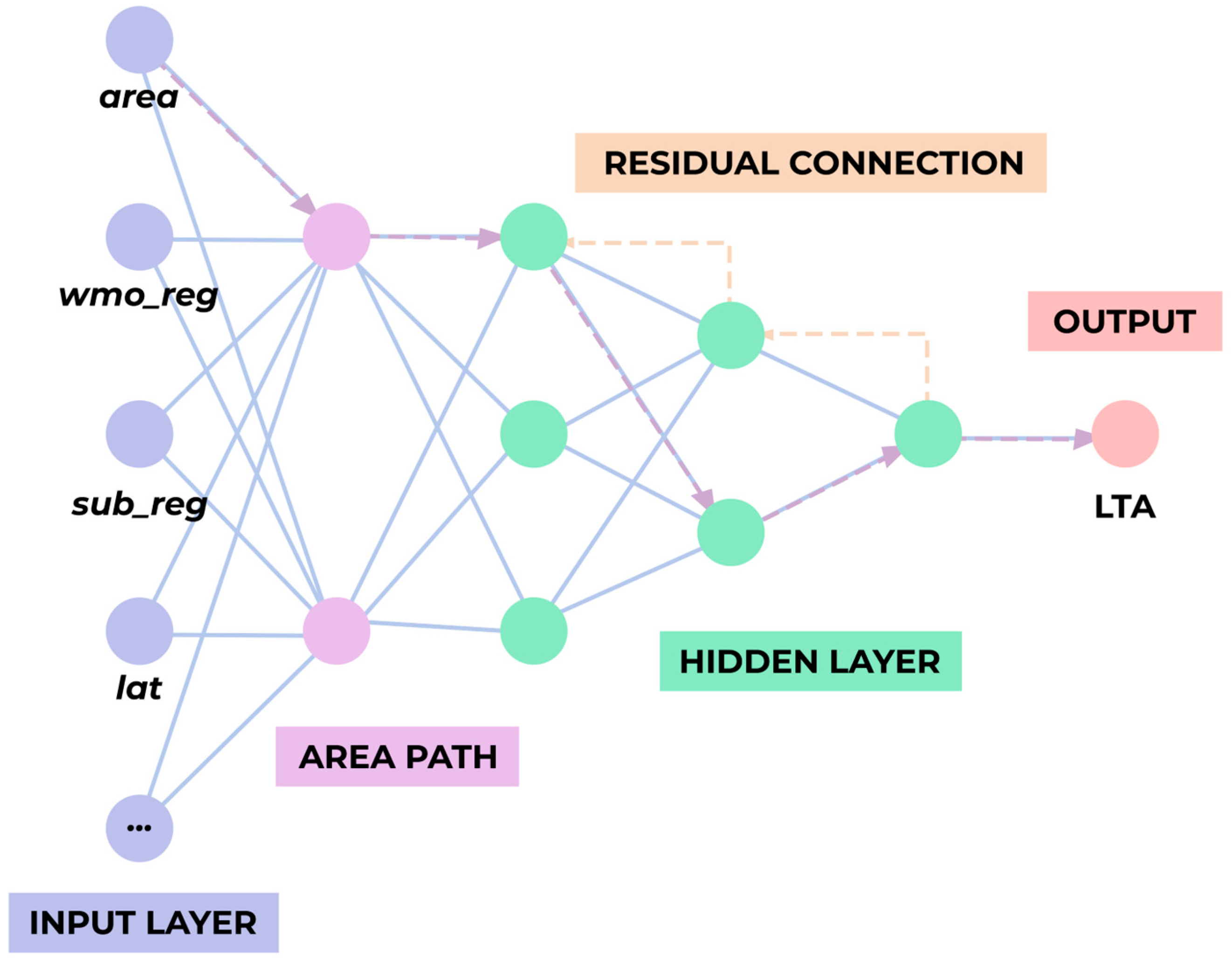
The developed Meta Ensemble model, which integrates predictions from an optimized Neural Network and several Gradient Boosting Machines, achieved excellent predictive performance on an independent test set (R² = 0.954, MAE = 71.3 m³/s). This significantly surpasses the accuracy of both baseline methods and individual advanced models, highlighting the power of hybrid ensembling for this hydrological task.

(2)

Model interpretability analysis using SHAP confirmed that the model learned physically plausible relationships. It identified catchment area as the most dominant predictor, with geographical location and regional identifiers playing a crucial secondary role in capturing spatial variability. This provides confidence that the model’s high accuracy is not a “black box” artifact but is grounded in hydrologically meaningful principles.

(3)

Rigorous data preprocessing and feature engineering were critical to the model’s success. The logarithmic transformation of the skewed target variable and the creation of interaction, ratio, and transformed geographical features were essential for achieving high performance.

(4)

The study demonstrates that it is feasible to build a robust and scalable tool for large-scale water resource assessment using readily available global metadata. This approach offers a valuable, cost-effective alternative to traditional methods, especially for preliminary assessments in ungauged or data-scarce basins.

In summary, this work contributes a robust methodology and a high-accuracy predictive model, advancing the application of machine learning in large-scale hydrology. It provides a validated framework for estimating a fundamental hydrological characteristic, offering a powerful tool to support global and regional water resource management and planning.

References

1. Zainuddin, A.A.; Hussin, A.A.A.; Annas, A.H.; Bharudin, M.S.; Razak, A.F.; Mahazir, M.N.B.; Puzi, A.A.; Handayan, D.; Raziff, A.R. Selective of IoT Applications for Water Quality Monitoring in Malaysia. Int. J. Percept. Cogn. Comput. 2024, 10, 8–16. [Google Scholar] [CrossRef]
2. González, L.; Gonzales, A.; González, S.; Cartuche, A. A Low-Cost IoT Architecture Based on LPWAN and MQTT for Monitoring Water Resources in Andean Wetlands. SN Comput. Sci. 2024, 5, 144. [Google Scholar] [CrossRef]
3. Raman, R.; Martin, N. IoT-Enabled Water Pollution Detection for Real-Time Monitoring and Pollution Source Identification with MQTT Protocol. In Proceedings of the 2024 International Conference on Advances in Data Engineering and Intelligent Computing 901 Systems (ADICS), Chennai, India, 18–19 April 2024; IEEE: Piscataway, NJ, USA, 2024; pp. 1–6. [Google Scholar] [CrossRef]
4. Galletti, A.; Avesani, D.; Bellin, A.; Majone, B. Detailed simulation of storage hydropower systems in large Alpine watersheds. J. Hydrol. 2019, 603, 127125. [Google Scholar] [CrossRef]
5. Farabi, M.R.; Sintawati, A. Flood Early Warning System at Jakarta Dam Using Internet of Things (IoT)-Based Real-Time Fishbone Method to Support Industry 4.0. J. Soft Comput. Explor. 2024, 5, 99–106. [Google Scholar] [CrossRef]
6. Dahane, A.; Benameur, R.; Naloufi, M.; Souihi, S.; Abreu, T.; Lucas, F.S.; Mellouk, A. IoT Urban River Water Quality System Using Federated Learning via Knowledge Distillation. In Proceedings of the 2024 IEEE International Conference on Communications (ICC 2024), Denver, CO, USA, 9–13 June 2024; IEEE: Piscataway, NJ, USA, 2024; pp. 1515–1520. [Google Scholar] [CrossRef]
7. Nordling, K.; Fahrenbach, N.L.; Samset, B.H. Climate variability can outweigh the influence of climate mean changes for extreme precipitation under global warming. Atmos. Chem. Phys. 2025, 25, 1659–1684. [Google Scholar] [CrossRef]
8. More, K.; Morey, U.; Motade, P.; Muchandi, A.; Motewar, S.; Mukkawar, K. GREEN GUARDIAN: IoT Driven Water Management for Sustainable Agriculture. In Proceedings of the 2024 2nd International Conference on Advances in Computation, Communication and Information Technology (ICAICCIT), Faridabad, India, 28–29 November 2024; IEEE: Piscataway, NY, USA, 2024; Volume 1, pp. 1354–1359. [Google Scholar] [CrossRef]
9. Promput, S.; Maithomklang, S.; Panya-isara, C. Design and Analysis Performance of IoT-Based Water Quality Monitoring System using LoRa Technology. TEM J. 2023, 12, 49–54. [Google Scholar] [CrossRef]
10. Majone, B.; Avesani, D.; Zulian, P.; Fiori, A.; Bellin, A. Analysis of high streamflow extremes in climate change studies: How do we calibrate hydrological models? Hydrol. Earth Syst. Sci. 2021, 26, 3863–3883. [Google Scholar] [CrossRef]
11. Kumar, M.; Singh, T.; Maurya, M.K.; Shivhare, A.; Raut, A.; Singh, P.K. Quality Assessment and Monitoring of River Water Using IoT Infrastructure. IEEE Internet Things J. 2023, 10, 10280–10290. [Google Scholar] [CrossRef]
12. Singh, J.; Srivastava, A.; Dalal, V. Designing of Real-time Communication Method to Monitor Water Quality using WSN Based on IoT. Int. J. Recent Innov. Trends Comput. Commun. 2023, 11, 437–446. [Google Scholar] [CrossRef]
13. Olatinwo, S.O.; Joubert, T.H. Resource Allocation Optimization in IoT-Enabled Water Quality Monitoring Systems. Sensors 2023, 23, 8963. [Google Scholar] [CrossRef]
14. Pires, L.M.; Gomes, J. River Water Quality Monitoring Using LoRa-Based IoT. Designs 2024, 8, 127. [Google Scholar] [CrossRef]
15. Nasution, S.F.; Harmadi, H.; Suryadi, S.; Widiyatmoko, B. Development of River Flow and Water Quality Using IoT-based Smart Buoys Environment Monitoring System. J. Ilmu Fisika Univ. Andalas 2023, 16, 1–12. [Google Scholar] [CrossRef]
16. Vaidya, R.; Bardekar, A.A. Analysis of Water Quality using IoT. J. Inf. Syst. Eng. Manag. 2025, 10, 1–7. [Google Scholar] [CrossRef]
17. Wang, L.; Cuia, S.; Lid, Y.; Huang, H.; Manandhar, B.; Nitivattananon, V.; Fang, X.; Huang, W. A review of the flood management: From flood control to flood resilience. Heliyon 2022, 8, e11763. [Google Scholar] [CrossRef]
18. Handini, W.; Widanti, N.; Lestari, S.W.; Haqq, A.R.; Hafizh, A.; Mulyadi, B. Design of Microhydro Power Plant Prototype by Utilizing Irrigation Water in Rice Fields Based on IoT. J. Penelit. Pendidik. IPA 2024, 10, 7144–7150. [Google Scholar] [CrossRef]
19. Ashley, M.; David, M.; Iriana, R. Pembuatan Prototype Alat Monitoring Kualitas Air Berbasis Internet of Things (IoT). J. Ilm. Tek. 2024, 3, 92–102. [Google Scholar] [CrossRef]
20. Akash, S.; Sahoo, S.; Vijayalakshmi, M. Enhancing High-Density Fish Farming in a Biofloc System Through IoT Driven Monitoring System. In Proceedings of the 2024 8th International Conference on Electronics, Communication and Aerospace Technology (ICECA), Coimbatore, India, 6–8 November 2024; IEEE: Piscataway, NY, USA, 2024; pp. 472–477. [Google Scholar] [CrossRef]
21. Nishan, R.K.; Akter, S.; Sony, R.I.; Hoque, M.M.; Anee, M.J.; Hossain, A. Development of an IoT-based multi-level system for real-time water quality monitoring in industrial wastewater. Discov. Water 2024, 4, 43. [Google Scholar] [CrossRef]
22. Ghorpade, A.M.; Nanaware, J.D. IoT Based Real Time Dam Water Level Monitoring System. J. Emerg. Technol. Innov. Res. 2020, 7, 266–269. [Google Scholar]
23. Souilmi, F.Z.; Ghedda, K.; Fahde, A.; Fihri, F.Z.; Tahraoui, S.; Elasri, F.; Malki, M. Taxonomic diversity of benthic macroinvertebrates along the Oum Er Rbia River (Morocco): Implications for water quality bio-monitoring using indicator species. Biodivers. Conserv. 2019, 27, 137–149. [Google Scholar]
24. Ahmed, M.A.; Li, S.S. Machine Learning Model for River Discharge Forecast: A Case Study of the Ottawa River in Canada. Hydrology 2024, 11, 151. [Google Scholar] [CrossRef]
25. Adeniyi, O.D.; Odigure, J.O. Water quality monitoring: A case study of water pollution in Minna and its environs in Nigeria. Botswana J. Technol. 2006, 14, 31–35. [Google Scholar] [CrossRef]
26. Lee, B.W.; Yoon, J.; Ko, D.; Song, H. Optimization of Structural Scales for Ripraps and Gabions at Seadike Closure. J. Coast. Res. 2024, 116, 6–10. [Google Scholar] [CrossRef]
27. Hebbache, M.; Zenati, N.; Belahcene, N.; Messadi, D.; Noureddine, Z. Impact of Hydraulic Developments on the Quality of Surface Water in the Mafragh Watershed, El Tarf, Algeria. Nat. Environ. Pollut. Technol. 2024, 23, 775–783. [Google Scholar] [CrossRef]
28. Asadollahi, A.; Magar, B.A.; Poudel, B.; Sohrabifar, A.; Kalra, A. Application of Machine Learning Models for Improving Discharge Prediction in Ungauged Watershed: A Case Study in East DuPage, Illinois. Geographies 2024, 4, 363–377. [Google Scholar] [CrossRef]
29. Fuentes-Peñailillo, F.; Ortega-Farías, S.; Acevedo-Opazo, C.; Rivera, M.; Araya-Alman, M. A Smart Crop Water Stress Index-Based IoT Solution for Precision Irrigation of Wine Grape. Sensors 2023, 24, 25. [Google Scholar] [CrossRef]
30. Georgantas, I.; Mitropoulos, S.; Katsoulis, S.; Chronis, I.; Christakis, I. Integrated Low-Cost Water Quality Monitoring System Based on LoRa Network. Electronics 2025, 14, 857. [Google Scholar] [CrossRef]
31. Wegehenkel, M.; Beyrich, F. Modelling hourly evapotranspiration and soil water content at the grass-covered boundary-layer field site Falkenberg, Germany. Hydrol. Sci. J. 2014, 59, 376–394. [Google Scholar] [CrossRef]
32. Majoro, F.; Wali, U.G.; Munyaneza, O.; Naramabuye, F.X.; Mukamwambali, C. On-site and Off-site Effects of Soil Erosion: Causal Analysis and Remedial Measures in Agricultural Land—A Review. RJESTE 2020, 3, 1–19. [Google Scholar] [CrossRef]
33. Behney, A.C. The Influence of Water Depth on Energy Availability for Ducks. J. Wildl. Manag. 2020, 84, 436–447. [Google Scholar] [CrossRef]
34. Huang, C.; Chang, C.; Chang, C.; Tsai, M. Development of a lightweight convolutional neural network-based visual model for sediment concentration prediction by incorporating the IoT concept. J. Hydroinform. 2023, 25, 2660–2674. [Google Scholar] [CrossRef]
35. Dimitriou, E.; Poulis, G.; Papadopoulos, A. Development of a water monitoring network based on open architecture and Internet-of-Things technologies. In Proceedings of the EGU General Assembly 2021, Online, 19–30 April 2021; p. EGU21-13460. [Google Scholar] [CrossRef]
36. Hahn, Y.; Kienitz, P.; Wönkhaus, M.; Meyes, R.; Meisen, T. Towards Accurate Flood Predictions: A Deep Learning Approach Using Wupper River Data. Water 2024, 16, 3368. [Google Scholar] [CrossRef]
37. Boonrat, P.; Boonrat, P.; Aharari, A. Precision Rehabilitation: IoT-Based Monitoring in Mangrove Ecosystems. In Proceedings of the 2024 IEEE 4th International Conference on Electronic Communications, Internet of Things and Big Data (ICEIB), Taipei, Taiwan, 19–21 April 2024; IEEE: Piscataway, NY, USA, 2024; pp. 145–149. [Google Scholar] [CrossRef]
38. Sudibyo, H.; Yuniko, F.T.; Fadel, A.; Lesmana, L.S.; Efendi, R. Sistem Monitoring Budidaya Perikanan Berbasis IoT Fish Feeder Sebagai Implementasi Smart Farming. JOISIE 2024, 8, 236–247. [Google Scholar] [CrossRef]
39. Boudville, R.; Tapah, J.B.; Yuzi, A.A.; Johan, N.A.; Daing, M.I.; Aliastar, N.A. Development of IoT-based Headwater Phenomenon Monitoring and Warning System. In Proceedings of the 2024 IEEE 14th International Conference on Control System, Computing and Engineering (ICCSCE), Penang, Malaysia, 23–24 August 2024; IEEE: Piscataway, NY, USA, 2024; pp. 232–236. [Google Scholar] [CrossRef]
40. Anda, M.; Fornarelli, R.; Dallas, S.; Schmack, M.; Byrne, J.; Morrison, G.M.; Fox-Reynolds, K. Ultrasonic Smart Metering: Realising the Benefits of Residential Hybrid Water Systems. In WEC2019: World Engineers Convention; Engineers Australia: Melbourne, Australia, 2019; pp. 927–938. [Google Scholar]
41. Don, A.A.; Felimar, T.L. Comparative Study of Intrusion Detection Systems against Mainstream Network Sniffing Tools. Int. J. Eng. Technol. 2018, 7, 188–191. [Google Scholar] [CrossRef]
42. Mahaasin, H.I.; Kusuma, P.D.; Hasibuan, F.C. Back-end website development for IoT-based automated water dissolved oxygen control. J. Comput. Eng. Progr. Appl. Technol. 2023, 2, 36–43. [Google Scholar] [CrossRef]
43. Rajashree, N.; Nithisha, Y.S.; Shaheen, S.; Govardhan, P. An IoT Approach for Monitoring Aqua Culture Using GSM Module. IRE Journals. 2020, 3, 284–288. [Google Scholar]
44. Miskon, M.T.; Makmud, M.Z.H.; Zacharee, M.; Abd Rahman, A.B. Real-Time Hardware-In-The-Loop Simulation of IoT-Enabled Mini Water Treatment Plant. In Proceedings of the 2024 IEEE International Conference on Automatic Control and Intelligent Systems (I2CACIS), Shah Alam, Malaysia, 29 June 2024; IEEE: Piscataway, NY, USA, 2024; pp. 319–324. [Google Scholar] [CrossRef]
45. Bărbulescu, A.; Zhen, L. Forecasting the River Water Discharge by Artificial Intelligence Methods. Water 2024, 16, 1248. [Google Scholar] [CrossRef]
46. Huang, J.; Chen, J.; Huang, H.; Cai, X. Deep Learning-Based Daily Streamflow Prediction Model for the Hanjiang River Basin. Hydrology 2025, 12, 168. [Google Scholar] [CrossRef]
47. Abdurrafi, A.; Maulana, D.; Kurniadi, N.T. Optimization Water Conservation Through IoT Sensor Implementation At Smartneasy Nusantara. J. Appl. Intell. Syst. 2023, 8, 432–441. [Google Scholar] [CrossRef]
48. Workneh, H.A.; Jha, M.K. Utilizing Deep Learning Models to Predict Streamflow. Water 2025, 17, 756. [Google Scholar] [CrossRef]
49. Ziadi, S.; Chokmani, K.; Chaabani, C.; El Alem, A. Deep Learning-Based Automatic River Flow Estimation Using RADARSAT Imagery. Remote Sens. 2024, 16, 1808. [Google Scholar] [CrossRef]
50. Liu, W.; Zou, P.; Jiang, D.; Quan, X.; Dai, H. Computing River Discharge Using Water Surface Elevation Based on Deep Learning Networks. Water 2023, 15, 3759. [Google Scholar] [CrossRef]
51. Francisco, R.; Matos, J.P. Deep Learning Prediction of Streamflow in Portugal. Hydrology 2024, 11, 217. [Google Scholar] [CrossRef]
52. Zhen, L.; Bărbulescu, A. Quantum Neural Networks Approach for Water Discharge Forecast. Appl. Sci. 2025, 15, 4119. [Google Scholar] [CrossRef]
53. Almaaitah, T.; Joksimovic, D.; Sajin, T. Real-Time IoT-Enabled Water Management for Rooftop Urban Agriculture Using Commercial Off-the-Shelf Products. Chem. Proc. 2022, 10, 34. [Google Scholar] [CrossRef]
54. Rosa, S.L.; Kadir, E.A.; Siswanto, A.; Othmand, M.; Daud, H. Identifying Water Pollution Sources Using Real-Time Monitoring and IoT. Int. J. Adv. Sci. Eng. Inf. Technol. 2022, 12, 2122–2131. [Google Scholar] [CrossRef]
55. Chowdurya, M.S.; Emran, T.B.; Ghosh, S.; Pathak, A.; Alam, M.M.; Absar, N.; Andersson, K.; Shahadat, M.; Hossain, S.; Subhasish, H. IoT-Based Real-Time River Water Quality Monitoring System. Procedia Comput. Sci. 2019, 155, 161–168. [Google Scholar] [CrossRef]
56. Chaarmart, K.; Jeebkaew, K.; Sripa, S.; Burtyothee, W. Solar Cells Powered Boat for Water Quality Monitoring of Nonghan River Using Wireless Sensor. J. Ind. Technol. Innov. 2024, 3, 254028. [Google Scholar] [CrossRef]
57. Youssef, S.B.; Rekhis, S.; Boudriga, N. A Blockchain-Based Secure IoT Solution for Dam Surveillance. In Proceedings of the 2019 IEEE Wireless Communications and Networking Conference (WCNC), Marrakesh, Morocco, 15–18 April 2019; IEEE: Piscataway, NY, USA, 2019; pp. 1–6. [Google Scholar] [CrossRef]
58. Dhandre, N.M.; Kamalasekaran, P.D.; Pandey, P. Dam Parameters Monitoring System. In Proceedings of the 2016 7th India International Conference on Power Electronics (IICPE), Patiala, India, 17–19 November 2016; IEEE: Piscataway, NY, USA, 2016; pp. 1–5. [Google Scholar] [CrossRef]
59. Sharifi, L.; Kamel, S.; Feizizadeh, B. Monitoring Bioenvironmental Impacts of Dam Construction on Land Use/Cover Changes in Sattarkhan Basin Using Multi-Temporal Satellite Imagery. Iran. J. Energy Environ. 2015, 6, 39–46. [Google Scholar] [CrossRef]
60. Chen, S.; Yang, H.; Zheng, H. Intercomparison of Runoff and River Discharge Reanalysis Datasets at the Upper Jinsha River, an Alpine River on the Eastern Edge of the Tibetan Plateau. Water 2025, 17, 871. [Google Scholar] [CrossRef]
61. BfG-GRDC Data Download. Available online: https://portal.grdc.bafg.de/applications/public.html?publicuser=PublicUser#dataDownload/StationCatalogue (accessed on 4 May 2025).
62. Yong, K.; Li, M.; Xiao, P.; Gao, B.; Zheng, C. Monthly Streamflow Forecasting for the Irtysh River Based on a Deep Learning Model Combined with Runoff Decomposition. Water 2025, 17, 1375. [Google Scholar] [CrossRef]
63. Irawan, B.; Fahmi, F.; Zamzami, E.M. Optimizing K-Nearest Neighbor Values Using The Elbow Method. In Proceedings of the 2024 Ninth International Conference on Informatics and Computing (ICIC), Medan, Indonesia, 24–25 October 2024; IEEE: Piscataway, NY, USA, 2024; pp. 1–4. [Google Scholar] [CrossRef]
64. Guo, H.; Liu, X.; Zhang, Q. Identifying Daily Water Consumption Patterns Based on K-Means Clustering, Agglomerative Hierarchical Clustering, and Spectral Clustering Algorithms. AQUA 2024, 73, 870–887. [Google Scholar] [CrossRef]
65. Szegedy, C.; Ioffe, S.; Vanhoucke, V.; Alemi, A.A. Inception-v4, Inception-ResNet and the Impact of Residual Connections on Learning. In Proceedings of the AAAI Conference on Artificial Intelligence, San Francisco, CA, USA, 4–9 February 2017; Volume 31, pp. 4278–4284. [Google Scholar] [CrossRef]
66. Chen, T.; Guestrin, C. XGBoost: A Scalable Tree Boosting System. In Proceedings of the 22nd ACM SIGKDD International Conference on Knowledge Discovery and Data Mining, San Francisco, CA, USA, 13–17 August 2016; ACM: Piscataway, NY, USA, 2016; pp. 785–794. [Google Scholar] [CrossRef]
67. Dolhopolov, S.; Honcharenko, T.; Terentyev, O.; Savenko, V.; Rosynskyi, A.; Bodnar, N.; Alzidi, E. Multi-Stage Classification of Construction Site Modeling Objects Using Artificial Intelligence Based on BIM Technology. In Proceedings of the 35th Conference of Open Innovations Association (FRUCT), Tampere, Finland, 24–26 April 2024; FRUCT: Helsinki, Finland, 2024; pp. 179–185. [Google Scholar] [CrossRef]
68. Zhang, L.; Jánošík, D. Enhanced Short-Term Load Forecasting with Hybrid Machine Learning Models: CatBoost and XGBoost Approaches. Expert Syst. Appl. 2024, 241, 122686. [Google Scholar] [CrossRef]
69. Zhou, Y.; Pan, J.; Shao, G. A Comparative Study of a Two-Dimensional Slope Hydrodynamic Model (TDSHM), Long Short-Term Memory (LSTM), and Convolutional Neural Network (CNN) Models for Runoff Prediction. Water 2025, 17, 1380. [Google Scholar] [CrossRef]
Figure 1. Global distribution of monitoring stations included in the GRDC dataset, illustrating geographical coverage and density variations across continents.
Water 17 02097 g001
Figure 2. Distribution histograms of monitoring stations highlighting the geographical spread and concentration areas: (a) latitude; (b) longitude.
Water 17 02097 g002
Figure 3. Bar chart showing the number of monitoring stations categorized by World Meteorological Organization (WMO) region, indicating regional monitoring density.
Water 17 02097 g003
Figure 4. Geographical distribution of monitoring stations in Eurasia, highlighting Kazakhstan and surrounding regions. Point size and color indicate long-term average discharge, illustrating hydrological variability.
Water 17 02097 g004
Figure 5. Distributions of key hydrological variables: (a) Long-term Average Discharge; (b) Mean Annual Runoff Volume.
Water 17 02097 g005
Figure 6. Distributions related to daily data records: (a) Record Length; (b) Start Year.
Water 17 02097 g006
Figure 7. Relationship between Daily Data Record Length and Missing Data Percentage. The scatter plot illustrates that many stations with long records maintain high data completeness.
Water 17 02097 g007
Figure 8. Analysis of scale-dependent hydrological relationship: (a) power-law relationship between Catchment Area and Long-term Average Discharge on a log-log scale; (b) relationship between Specific Discharge and Catchment Area.
Water 17 02097 g008
Figure 9. Elbow method plot showing the sum of squared distances versus the number of clusters (k), used to determine an optimal k for clustering.
Water 17 02097 g009
Figure 10. Spatial distribution of monitoring stations colored by cluster assignment (k = 5), illustrating geographical groupings.
Water 17 02097 g010
Figure 11. Correlation matrix heatmap for the top 15 features most correlated with the target variable.
Water 17 02097 g011
Figure 12. Hierarchical clustering of hydrological variables based on their correlation matrix.
Water 17 02097 g012
Figure 13. Bar chart showing feature importance scores derived from an initial XGBoost model.
Water 17 02097 g013
Figure 14. Architecture of the Advanced Neural Network, detailing the input layer, specialized path for the “Area” feature, hidden layers with neuron counts, residual connections, and the final output layer predicting LTA Discharge.
Water 17 02097 g014
Figure 15. Architecture of the Meta Ensemble model, showing inputs feeding into individual models (Neural Network, Neural Ensemble, XGBoost, LightGBM, CatBoost), the predictions of which are weighted and combined in the Meta Ensemble layer to produce the final prediction.
Water 17 02097 g015
Figure 16. Bar chart comparing Training R2 and Testing R2 scores across different models. The dashed green line indicates the target R2 performance of 0.9.
Water 17 02097 g016
Figure 17. Comparison of Root Mean Squared Error (RMSE) on the logarithmic scale across all evaluated models. Lower values indicate better performance.
Water 17 02097 g017
Figure 18. Mean Absolute Error (MAE) on the original discharge scale (m3/s) across all evaluated models, plotted with a logarithmic y-axis. Lower values indicate better performance.
Water 17 02097 g018
Figure 19. Predicted vs. actual values for the final Meta Ensemble model on the test set: (a) comparison on a logarithmic scale; (b) comparison on the original discharge scale (m3/s). Points are colored by absolute error.
Water 17 02097 g019
Figure 20. Residual analysis plots for the Meta Ensemble model on the test set (logarithmic scale): (a) residuals vs. predicted values; (b) histogram of residuals; (c) density plot of residuals; (d) Q-Q plot of residuals.
Water 17 02097 g020
Figure 21. SHAP summary plot (beeswarm plot) illustrating global feature importance. Each point represents a Shapley value for a feature and an instance. The position on the y-axis is determined by the feature, and on the x-axis by the Shapley value.
Water 17 02097 g021
Figure 22. SHAP dependence plot for the most important feature, area_log. It shows the feature’s value on the x-axis and its corresponding SHAP value (impact on model output) on the y-axis. The color corresponds to the value of a second, interacting feature (lat).
Water 17 02097 g022
Figure 23. SHAP waterfall plot for a single prediction, showing how the positive and negative contributions of each feature sum up to produce the final prediction from the base value.
Water 17 02097 g023
Figure 24. Example time series visualization showing a multi-year overview (2015–2025) of water discharge at three hypothetical monitoring stations. The plot illustrates long-term patterns, seasonal cycles, and relative differences in flow magnitude.
Water 17 02097 g024
Figure 25. Detailed time series visualization focusing on the first year (2015) of water discharge data from the three stations, highlighting seasonal patterns and short-term variability.
Water 17 02097 g025
Figure 26. Conceptual architecture of a potential integrated water resources monitoring system where the developed LTA estimation model could be deployed.
Water 17 02097 g026
Figure 27. Conceptual flowchart of an integrated operational monitoring algorithm, illustrating the potential deployment workflow for the LTA estimation model.
Water 17 02097 g027