Numerical Simulation of Hydrodynamic Characteristics for Monopile Foundations of Wind Turbines Under Wave Action

Abstract

The calculation and evaluation of wave loads represent a critical component in the design process of offshore wind turbines, which is of significant value for ensuring the safety and stability of offshore wind turbines during operation. In recent years, as the offshore wind power industry has extended into deep-sea areas, wind turbines and their foundation structures have gradually increased in scale. Due to the continuously growing diameter of fixed foundation structures, the wave loads they endure can no longer be evaluated solely by traditional methods. This study simplifies the monopile foundation structure of wind turbines into an upright circular cylinder. The open-source CFD platform OpenFOAM is employed to establish a numerical wave tank, and large eddy simulation (LES) models are used to conduct numerical simulations of its force-bearing process in wave fields. Through this approach, the hydrodynamic loads experienced by the single-cylinder structure in wave fields and the surrounding wave field data are obtained, with further investigation into its hydrodynamic characteristics under different wave environments. By analyzing the wave run-up distribution around cylinders of varying diameters and their effects on incident waves, a more suitable value range for traditional theories in engineering design applications is determined. Additionally, the variation laws of horizontal wave loads on single-cylinder structures under different parameter conditions (such as cylinder diameter, wave steepness, water depth, etc.) are thoroughly studied. Corresponding hydrodynamic load coefficients are derived, and appropriate wave force calculation methods are established to address the impact of value errors in hydrodynamic load coefficients within the transition range from large-diameter to small-diameter cylinders in traditional theories on wave force evaluation. This contributes to enhancing the accuracy and practicality of engineering designs.

1. Introduction

In the recent three decades, the international energy supply has become increasingly strained, and environmental pollution issues have grown more severe. In response to this worsening energy crisis, countries have recognized the importance of developing renewable clean energy. Wind power generation, an important means of accessing clean energy, can be divided into onshore and offshore development models. In recent years, offshore wind power has gradually elevated its status in the global energy landscape [1]. Currently, the offshore wind power industry is continuously developing toward large-scale, deep-water, and intelligent directions [2]. The development of deep-water wind farms with large-capacity wind turbines and floating foundations has become a research hotspot in both engineering and academic circles [3,4,5], and how to balance structural costs with safety and stability is also one of the key issues of common concern. To address this problem, accurately evaluating the hydrodynamic loads on support structures is a critical aspect that cannot be overlooked. Therefore, when engaging in work related to the development and utilization of offshore wind farms, studying the hydrodynamic load characteristics of support structures holds significant importance.

In marine environments, loads generated by waves and currents have a significant impact on the stability of wind turbine foundations [6,7,8]. These loads exert forces such as drag force, inertial force, and diffraction force on the foundation through mechanisms like wave impact, vortex shedding induced by turbulence, and water flow motion [9]. The substructure of offshore wind turbine foundations typically adopts a single cylindrical column or a combined form of multiple cylindrical columns. For such structures, there are two classic theoretical models for calculating wave forces: Morison’s equation and diffraction theory. These two calculation methods have different application conditions in practical engineering, with their applicable ranges depending on the size characteristics of the cylindrical structure, specifically expressed as the ratio $D/L$ of the pile diameter D to the corresponding wave wavelength L. In international general design codes, the definition of small-diameter cylinders is specified: when $D/L<0.2$, the horizontal component force expression of the cylinder is completely consistent with Morison’s equation; when $D/L>0.2$, the cylinder is considered a large-diameter cylinder, and the diffraction effect occurring in the wave field must be considered during calculations [10].

For small-diameter piles, Keulegan and Carpenter discovered a close correlation between the drag coefficient $C_D$, inertia coefficient $C_M$, and the Keulegan–Carpenter (KC) number. To gain a deeper understanding of this phenomenon, Fourier analysis was employed to conduct a detailed exploration of experimental data, yielding average values for $C_D$ and $C_M$. Further analysis revealed that these two coefficients are actually functions of the Reynolds number Re, KC number, relative roughness $k^{*}/D$, and time t. Coakrabarti proposed a general form of the wave force equation for submerged or semi-submerged small-diameter cylinders, which serves as an extension of Morison’s equation. Through least squares analysis of experimentally measured force data, hydrodynamic coefficients in the form of $C_D$ and $C_M$ were obtained for the generalized Morison equation. Multiple tests were conducted, and experimental data were normalized to provide hydrodynamic coefficient values. Yun [11] simplified the traditional Morison equation and derived a simplified second-order nonlinear Morison equation based on second-order Stokes waves. Meanwhile, the accuracy of the simplified Morison equation was validated, and a stable point method was proposed to solve second-order nonlinear wave forces. Iwagaki [12] conducted experimental studies under wave–current coexisting conditions, expressing coefficients $C_D$ and $C_M$ as functions of the KC number. Kato [13] investigated the wave force characteristics on vertical cylinders through oscillating cylinder experiments in a wave tank, indicating that the oscillation frequency has a significant impact on the inertia coefficient $C_M$. Zan [14] found that inertia and drag coefficients affect the characteristics of the velocity field. The results show that in the upper and lower layers, stratification-related empirical coefficients can improve the performance of Morison’s equation, but there is no obvious advantage in layers close to the density interface.

Unlike small-diameter cylinders, large-diameter cylinders significantly affect the surrounding wave field, with fluid motion being strongly disturbed, leading to wave reflection and diffraction phenomena. Diffraction theory is based on potential flow theory and linear wave theory. Although it has a theoretically rigorous foundation, its limitations are particularly evident in practice. First, diffraction theory has limited applicability. In practical applications, analytical solutions can only be obtained for simple structural geometries. Second, its calculation accuracy is insufficient for nonlinear wave conditions, as second-order diffraction forces and other nonlinear effects introduce significant errors. While higher-order methods can improve accuracy, their complex computational processes and practical application challenges have limited the development of diffraction theory in engineering. To address the difficulties in solving second-order wave diffraction problems for large vertical cylinders, researchers have provided second-order potential theory solutions for the free surface in first- and second-order diffraction problems, and derived second-order radiation potentials under far-field radiation conditions. Teng [15] proposed a forward prediction method for calculating free surface integrals for second-order potentials, using different techniques to handle singularities in the surface and volume integrals of the ring Green’s function. This was validated by comparing second-order forces, moments, and diffraction effects on cylindrical structures. Molin [16] studied third-order wave forces on vertical cylinders under finite water depth conditions, finding that long-wave theory is inapplicable for third-order force calculations when compared with experimental results. Hiao [17] used the boundary element method to compute unsteady wave surface potentials for large structures in combined wave–current fields, employed the surface vorticity method to analyze flow velocity changes around structures, and obtained first-order wave forces on large structures under current action.

This thesis simplifies the wind turbine foundation structure as a vertical cylindrical structure to study the hydrodynamic characteristics of vertical cylinders in wave fields. Computational fluid dynamics (CFD) methods are employed to simulate the interaction between waves and cylindrical structures, acquiring flow field information and horizontal force data under wave action [18,19,20]. By comparing with experimental data from laboratory physical model tests, the simulation results of wave–structure interaction under different grid conditions are evaluated, and the optimal grid ratio for model calculation is determined to validate the reliability and accuracy of the numerical model. The influence of diffraction effects on cylindrical structures with different diameters in regular wave fields is analyzed. The impacts of cylinders on wave fields under pure wave conditions and combined wave–current conditions are simulated, and the variation laws of wave run-up on the cylindrical wall, as well as the reflection and transmission effects of cylinders on surrounding wave fields, are studied. Additionally, the changes in the vorticity field around the cylinder are analyzed to obtain the vorticity variation laws for cylinders of different diameters, and the wave field changes in the transition interval between large- and small-diameter cylinders are explored to provide a basis for better distinguishing between large- and small-diameter cylinders. Subsequently, the results are compared with empirical outcomes from Morison’s equation and diffraction theory in engineering practice to determine the error patterns. Through least squares fitting of wave force data, the hydrodynamic load coefficients of wave forces on cylinders in numerical simulations are calculated, and engineering application formulas are modified using hydrodynamic load coefficients fitted from extensive results. The influence range of the diffraction effect on the wave field was determined by considering the effects of different diameters, wave heights, and flow velocities. Based on this, cylindrical structures with various diameters were defined, and the problems of boundary distinction between large and small diameters of cylinders and the applicability of nonlinear wave loads in traditional theories were corrected.

2. Methods

This study employs the open-source CFD software OpenFOAM v2206, based on the finite volume method, for hydrodynamic analysis of offshore wind turbine facilities. OpenFOAM is a C++-based CFD package with multiple solvers for various fluid mechanics problems, or custom solvers/tools can be developed. It includes pre- and post-processing interfaces, ensuring consistent data transfer across different computing environments.

2.1. Turbulence Model

This study addresses the wave motion of a constant-temperature, unsteady, incompressible viscous fluid. The motion of the fluid medium satisfies the continuity equation and the momentum conservation equation, whose tensor forms in the Cartesian coordinate system are as follows [21]:

$${\displaystyle \frac{\partial u_i}{\partial x_i}}=0$$

(1)

$${\displaystyle \frac{\partial u_i}{\partial t}}+{\displaystyle \frac{\partial }{\partial x_j}}(u_i{u}_j)=-{\displaystyle \frac{1}{\rho }}{\displaystyle \frac{\partial p}{\partial x_i}}+{\displaystyle \frac{1}{\rho }}{\displaystyle \frac{\partial }{\partial x_j}}(\mu {\displaystyle \frac{\partial u_i}{\partial x_j}})$$

(2)

where $\rho$ denotes the fluid density; $i,j=\mathrm{1,2},3$ represent the three directions $x$, $y$, $z$ of the three-dimensional flow field, respectively; and $u_i$, $u_j$ are the components of the fluid velocity in the $x_i$ and $x_j$ directions, respectively.

This study employs the large eddy simulation (LES) model provided by OpenFOAM to simulate turbulent flows. Large eddy simulation reduces computational complexity by resolving large-scale turbulent structures in fluid flow through the model, offering high accuracy and computational efficiency, which has made it widely used in turbulence simulations. In the LES turbulence model, turbulent motions larger than the grid scale are directly calculated using the Navier–Stokes (N-S) equations, while the influence of small-scale vortices on large-scale motions is accounted for through approximate modeling. To distinguish between large-scale and small-scale motions, a mathematical filter function is established, which decomposes each variable into two parts. For any instantaneous fluid variable $\varphi$, it can be expressed as

$$\varphi =\overline{\varphi }+\varphi \prime$$

(3)

where $\overline{\varphi }$ is the large-scale averaged component, called the filtered variable, which is directly calculated by LES. $\varphi \prime$ is the small-scale component, reflecting the influence of small-scale motions on $\varphi$, also known as the subgrid-scale component of $\varphi$. The filtered large-scale component can be expressed as

$$\overline{\varphi }(x,t)={\int }_{D}G(x,x\prime )\varphi (x\prime ,t)dx\prime$$

(4)

where D is the control domain of the flow, $x\prime$ is the spatial coordinate in the actual flow region, $x$ is the spatial coordinate in the filtered large-scale space, and $G(x,x\prime )$ is the Gaussian filter function, which determines the scale for resolving vortices, thereby separating large eddies from small eddies. Vortices smaller than the filter function’s scale are filtered out, so the filtered Navier–Stokes (N-S) equations describing the incompressible large eddy flow field can be expressed as

$${\displaystyle \frac{\partial \overline{u_i}}{\partial x_i}}=0$$

(5)

$${\displaystyle \frac{\partial {\overline{u}}_i}{\partial t}}+{\overline{u}}_j{\displaystyle \frac{\partial {\overline{u}}_i}{\partial x_j}}=-{\displaystyle \frac{1}{\rho }}{\displaystyle \frac{\partial \overline{p}}{\partial x_i}}+{\displaystyle \frac{\partial }{\partial x_j}}\left(\upsilon {\displaystyle \frac{\partial {\overline{u}}_i}{\partial x_j}}\right)+{\displaystyle \frac{1}{\rho }}{\displaystyle \frac{\partial {\tau }_{ij}}{\partial x_j}}$$

(6)

$${\tau }_{ij}={\overline{u}}_i{\overline{u}}_j-\overline{u_i{u}_j}$$

(7)

where $\overline{u_i}$, $\overline{u_j}$ are the filtered velocity components, $\overline{p}$ is the filtered pressure, $x$ is the spatial position coordinate, t is time, $\nu$ is the kinematic viscosity, $\rho$ is the fluid density, and ${\tau }_{ij}$ is the subgrid-scale (SGS) stress, which captures the effect of the filtered small eddies on large eddy motions through the introduction of an additional stress term in the equation.

There are three commonly used turbulent subgrid-scale models for large eddy simulation: the Smagorinsky model, the dynamic model, and the WALE model. One shortcoming of the Smagorinsky Subgrid Scale model is that it contains a model coefficient, Cs, that is not universal and depends on the local flow conditions. Therefore, this model should be avoided for complex flows near walls and other intricate flow scenarios. Although the dynamic model adjusts Cs dynamically, it may still overestimate the turbulent viscosity in extremely near-wall regions (such as the viscous sublayer), requiring further correction by combining with wall models. Additionally, the extra implementation of test filtering and solving the Cs equations increases computational load and storage requirements. In the Wall-adapting Local Eddy–Viscosity (WALE) model, the eddy viscosity naturally drops to zero, eliminating the need for dynamic constant adjustment or damping functions to calculate wall-bounded flows, and it can detect all turbulent structures related to kinetic energy dissipation. Since the WALE model produces zero viscosity and can reproduce the laminar-to-turbulent transition, the WALE model is adopted as the turbulent subgrid-scale model in this study.

Subgrid-scale turbulence models typically employ the Boussinesq hypothesis and use the following approach to compute the SGS stress [22,23]:

$${\tau }_{ij}-{\displaystyle \frac{1}{3}}{\tau }_{kk}{\delta }_{ij}=-2{\mu }_t{\overline{S}}_{ij}$$

(8)

where the second term on the left-hand side, $-{\displaystyle \frac{1}{3}}{\tau }_{kk}{\delta }_{ij}$, is introduced to ensure the natural satisfaction of the incompressible fluid continuity equation. ${\mu }_t$ represents the subgrid-scale eddy viscosity. In the WALE model, the eddy viscosity model is given by

$${\mu }_t=\rho {\Delta }_s^2{\displaystyle \frac{(S_{ij}^d{S}_{ij}^d{)}^{3/2}}{({\overline{S}}_{ij}{\overline{S}}_{ij}{)}^{5/2}+(S_{ij}^d{S}_{ij}^d{)}^{5/4}}}$$

(9)

$$\begin{array}{c}{S}_{ij}^d={\displaystyle \frac{1}{2}}\left({\overline{g}}_{ij}^2+{\overline{g}}_{ji}^2\right)-{\displaystyle \frac{1}{3}}{\delta }_{ij}{\overline{g}}_{kk}^2\end{array}$$

(10)

$${\overline{S}}_{ij}={\displaystyle \frac{1}{2}}\left({\displaystyle \frac{\partial {\overline{u}}_i}{\partial x_j}}+{\displaystyle \frac{\partial {\overline{u}}_j}{\partial x_i}}\right)$$

(11)

$${\Delta }_s=C_w{V}^{1/3}$$

(12)

where ${\overline{S}}_{ij}$ is the strain rate tensor of the resolved scale, and ${\Delta }_s=C_w{V}^{1/3}$ is the characteristic filter length, defined as the cube root of the grid cell volume (related to the grid size), with the constant $C_w=0.325$, ${\overline{g}}_{ij}={\displaystyle \frac{\partial \overline{u_i}}{\partial x_j}}$ and ${\overline{g}}_{ij}^2={\overline{g}}_{ik}{\overline{g}}_{kj}$.

2.2. Numerical Processing Methods

This study employs the finite volume method (FVM) for discretization. This method performs discretization by subdividing the computational domain into numerous grids, ensuring each grid node is surrounded by an independent, non-overlapping control volume. Differential equations (i.e., governing equations) are then solved for each control volume, and a series of discretized equations are constructed through integration. In these discrete equations, unknowns are primarily concentrated at grid nodes as dependent variables. During the solution process, reasonable assumptions about the variation of dependent variables between grid nodes are required. From the perspective of selecting integration regions, the finite volume method can be regarded as an application of the subdomain method within the method of weighted residuals. The core idea of the subdomain method is to integrate the governing equations over small-scale subdomains and obtain solutions for the entire domain through interpolation, which aligns with the finite volume method. In terms of unknown solution approximation, it belongs to methods that use local approximation for discretization. By observing physical phenomena within control volumes, this method approximates unknown solutions locally to reduce computational complexity. In summary, the basic approach of the finite volume method combines the domain partitioning concept of the subdomain method with the approximate solution strategy of discretization, enabling effective numerical solutions for complex fluid dynamics problems.

The pressure–velocity coupling uses the PISO (Pressure Implicit with Splitting of Operators) algorithm, which calculates pressure by splitting implicit operators into multiple steps. The PISO algorithm is based on the fundamental principles of the SIMPLE algorithm but derives an accurate pressure equation—rather than an approximate pressure correction equation—through discretization of the continuity and momentum equations. Additionally, the PISO algorithm employs a predictor–corrector–recorrector iterative strategy, achieving second-order accuracy in time and suitability for unsteady flow calculations. By adopting three steps within a single iteration, the PISO algorithm accelerates convergence and demonstrates significant advantages in transient problem analysis.

For the discretization scheme of the momentum equation, the second-order upwind differencing scheme is used, which can accurately simulate fluid motion and effectively reduce numerical errors. When the grid structure of the flow domain aligns with the flow direction (e.g., simulating laminar flow in hexahedral grids), first-order accuracy discretization is acceptable. In such cases, numerical errors introduced by first-order methods are small and do not significantly affect simulation results. However, in practical simulations, it is difficult to perfectly align the grid structure with the flow direction. When fluid flows obliquely across grid lines, first-order methods lead to large discretization errors and manifest as numerical diffusion. Such errors cause simulation results to deviate from real-world behavior. Therefore, using a second-order accuracy method for momentum equation discretization significantly reduces discretization errors in scenarios with oblique grid-line crossing, enhancing simulation capability and accuracy.

2.3. Data Analysis Methods

This study uses the least squares method in time-domain analysis for hydrodynamic coefficient analysis, determining the values of hydrodynamic coefficients by minimizing the sum of squared deviations between the measured wave force $F_X\left(t\right)$ on the cylinder and the calculated wave force $F\left(t\right)$. In the study of small-diameter cylinders, the horizontal component force along the wave propagation direction is integrated along the water depth according to Morison’s equation to obtain the calculated total force on the cylinder in the flow direction:

$$F_c(t)=\int f(z,t)dz$$

(13)

By selecting appropriate inertial force coefficient $C_D$ and velocity force coefficient ${ C}_D$, the above equation can be written in the following form:

$$F_c\left(t\right)=C_{D}X\left(t\right)+C_{M}Y\left(t\right)$$

(14)

where

$$X(t)={\displaystyle \frac{1}{2}}\rho D\int U(z,t)|U(z,t)|dz$$

(15)

$$Y(t)=\rho {\displaystyle \frac{\pi D^2}{4}}\int {\displaystyle \frac{\partial U(z,t)}{\partial t}}dz$$

(16)

Let the total force obtained from the numerical simulation be $F_m\left(t\right)$, then the sum of squared errors between the two is

$$Q=\sum _{i=1}^N[(F_c(t)-F_m(t){]}^2=\sum _{i=1}^N[(C_{D}X(i)+C_{M}Y(i)-F_m(i){]}^2$$

(17)

In the formula, N denotes the number of measured data points, and i represents the value at the i-th moment. The values of ${ C}_D$ and $C_M$ are chosen to minimize Q. At this minimum, $\partial Q/C_D=\partial Q/C_M=0$, leading to

$$A_1{C}_D+A_2{C}_M=A_4$$

(18)

$$A_2{C}_D+A_3{C}_M=A_5$$

(19)

where $A_1=\Sigma X^2\left(i\right)$, $A_2=\Sigma X\left(i\right)Y\left(i\right)$, $A_3=\Sigma Y\left(i\right)$, $A_4=\Sigma F_m\left(i\right)X\left(i\right)$, and $A_5=\Sigma F_m\left(i\right)Y\left(i\right)$.

From this, we can derive

$$C_D=\left|\begin{array}{cc}{A}_4& A_2\\ A_5& A_3\end{array}\right|/\left|\begin{array}{cc}{A}_1& A_2\\ A_2& A_3\end{array}\right|$$

(20)

$$C_M=\left|\begin{array}{cc}{A}_1& A_4\\ A_2& A_5\end{array}\right|/\left|\begin{array}{cc}{A}_1& A_2\\ A_2& A_3\end{array}\right|$$

(21)

In the study of wave forces on large-diameter cylinders, the diffraction theory can be expressed as Morison’s equation, containing only the inertial force term. As shown in Equation (22), the horizontal wave force obtained by the linear diffraction theory can derive the inertial force coefficient in the diffraction flow regime shown in Equation (23). The inertial force coefficients corresponding to wave forces on cylinders of different diameters can be obtained through Equation (23). The application principle of the least squares method is similar to this, so there is no need to elaborate further.

$$F_x=\int d{F}_x=\rho C_{M}A{\int }_{-h}^{\eta }{\displaystyle \frac{\partial u_x}{\partial t}}dz$$

(22)

$$C_M={\displaystyle \frac{F_x}{\rho }}A{\int }_{-h}^{\eta }{\displaystyle \frac{\partial u_x}{\partial t}}dz$$

(23)

To calculate wave forces using Morison’s equation, it is necessary to obtain the velocities and accelerations of water particles in the theoretical flow field. This study introduces the wave surface equation $\eta$ and the horizontal velocity component $u$ of water particles given by the second-order Stokes wave theory.

$$\eta =A\left[-{\displaystyle \frac{Ak}{2sinh2kh}}+cos\theta +{\displaystyle \frac{Ak}{4}}{\displaystyle \frac{coshkh\left(2cos{h}^{2}kh+1\right)}{sin{h}^{3}kh}}cos2\theta \right]$$

(24)

$$u=A\omega \left[{\displaystyle \frac{coshk(z+h)}{sinhkh}}\mathit{cos}\theta +{\displaystyle \frac{3}{4}}Ak{\displaystyle \frac{cosh2k(z+h)}{sin{h}^{4}kh}}\mathit{cos}2\theta \right]$$

(25)

where $\theta =kx-\omega t$, $x$ and $z$ are the horizontal and vertical coordinates, respectively, and the still water level is at $z=0$.

Before calculating ${ C}_D$ and ${ C}_M$, the streamwise wave forces obtained from numerical simulations are first subjected to phase-averaging over 10 cycles. Subsequently, through analytical calculations, the relationships between the hydrodynamic coefficients ${ C}_D$, $C_M$ of the cylinder’s streamwise wave force, the KC number (where the KC number is defined by the water particle velocity at $z=0$, and $D/L$ are obtained. The fitting effect using the least squares method is shown in Figure 1. It can be seen from Figure 1 that the curve fitted by OLS highly coincides with the numerical simulation result, which verifies the effectiveness of OLS in solving hydrodynamic coefficients.

Fast Fourier Transform (FFT) is a widely used spectrum analysis technique applicable to both continuous and discrete signals. This study employs the FFT algorithm to carry out spectrum analysis on the data, where the specific algorithm of $Y=fft\left(X,n\right)$ is as follows:

$$X(k)=\sum _{j=1}^{N}x(j){\omega }_n^{(j-1)(k-1)}$$

(26)

where in the equation, ${\omega }_N={\omega }^{(-2\pi i)/N}$ represents the N-th harmonic frequency.

By invoking the function $Y=fft\left(X,n\right)$ to perform Fast Fourier Transform (FFT) on the discrete signal sequence X, n points represented in complex form can be obtained. It should be noted that if the number of points in the original signal sequence X is less than n, the function will automatically pad zeros at the end of the sequence until the requirement of n points is met; conversely, if the number of points in the original signal sequence X exceeds n, the $Y=fft\left(X,n\right)$ function will automatically truncate the excess points to ensure computational efficiency and meet specific requirements.

In order to save computational resources, the range of wave forces on the cylinder calculated in this thesis is approximately within 10 to 15 periods after the stable section. This length is relatively short for spectral analysis. Spectral analysis is a crucial step in signal processing, and the accuracy of its results directly affects the reliability of subsequent applications. Therefore, when performing spectral analysis, it is necessary to ensure that the length of the original data time series is at least 100 times the period of the signal to be analyzed. To meet this requirement, 12 periods were selected after the stable section for repeated concatenation until the time series length exceeded 100 times the period. Through comparison, it was found that when the length of the data time series was approximately 120 periods, the results obtained by Fast Fourier Transform (FFT) were the most accurate. Therefore, a time series consisting of 120 periods was used as the input data in the FFT analysis. Figure 2 shows the intuitive results of FFT applied to the wave forces on a large-diameter cylinder with $D/L=0.5$, revealing the magnitude and distribution of wave forces at different frequencies. Through in-depth analysis of these results, the intrinsic laws and characteristics of the wave forces on the cylinder can be further revealed, providing a strong foundation for subsequent data processing and applications.

3. Establishment and Validation of Numerical Model

To investigate the hydrodynamic characteristics around the wind turbine foundation under finite water depth conditions with varying solidity Sn and wave heights, two sets of working conditions are established.

As shown in Figure 3, a numerical wave tank is established, with a wave generation zone and a wave absorption zone set at the front and rear ends, respectively. The wave generation zone is used to produce waves and maintain their stability, while the wave absorption zone dissipates wave energy and reduces the impact of wave reflection on the computational domain. The middle part of the tank is the experimental zone, where waves freely propagate, evolve, and interact with structures. The X-axis is set to coincide with the wave propagation direction, the Y-axis is perpendicular to the still water surface and aligned with the cylinder direction, and the Z-axis is perpendicular to the side walls of the water tank.

This paper uses the waves2Foam tool in OpenFOAM software v2206 for wave generation and absorption [24]. As a plug-in for OpenFOAM, it exhibits excellent compatibility and a wide range of applications. In this study, wave generation and absorption are achieved using a relaxation zone model combined with a velocity inlet wave generation method and a sponge layer damping wave absorption method. When specifically applied to calculations, appropriate wave theories need to be selected according to different working conditions and wave parameters such as water depth, wave height, and period.

3.1. Grid Division and Boundary Setting

To ensure the accuracy and reliability of calculation results, hexahedral meshes are selected as the basic units of the flow field mesh. To balance computational accuracy and speed, mesh refinement is required around the cylinder and in the splash zone near the free water surface, enabling more precise capture of fluid motion details in this region and yielding more accurate calculation results.

The mesh division of the entire numerical wave tank is shown in Figure 4. O-type meshing is adopted for the area around the wind turbine foundation, with radial mesh refinement based on a dimensionless wall distance ${ y}^{+}\approx 1$. Regions farther from the cylinder are arranged with conventional mesh refinement levels. Within the entire numerical tank, the mesh is uniformly distributed along the X direction, while the mesh in the Y-axis direction is also uniformly distributed within the splash zone. For submerged parts and gas phase parts far from the splash zone, the mesh height gradually increases with a growth rate of 1.1, balancing computational accuracy and efficiency while ensuring continuity and transition of the overall mesh. The number of mesh elements in the fluid region of the entire water tank varies in the range of $2.0\times 10^6~7.6\times 10^6$ across different working conditions.

For the numerical wave tank, the inlet boundary obtains the initial wave velocity based on wave theory, while the outlet boundary is set as a velocity–pressure outlet boundary with a zero gradient for velocity and pressure, where the pressure equals atmospheric pressure. Since the inlet and outlet boundary meshes lack geometric topological information, they are designated as patches. The upper and lower interfaces of the numerical tank are set to adopt no-slip, no-penetration solid wall boundary conditions (wall). The side boundary conditions use slip boundaries, and the surface of the wind turbine foundation is also set to solid wall boundary conditions.

The numerical wave generation and absorption adopt the method improved by Jacobsen [25] and Paulsen [26], which combines the velocity boundary wave generation method with the sponge layer damping wave absorption method to establish a relaxation zone model. This relaxation zone is distributed at the front and rear ends of the numerical wave tank, serving both functions, of wave generation and wave absorption. Through this improved method, a flow field fully consistent with the target wave theory is generated at the inlet boundary of the numerical tank. During propagation through the relaxation zone, it gradually transitions to being governed by the Navier–Stokes equations. The calculation results of the Navier–Stokes equations are then progressively corrected based on the target wave field to achieve the goal of wave generation. The implementation method is shown in the following equation:

$$U=\epsilon U_{target}+(1-\epsilon )U_{computed}$$

(27)

$$\alpha =\epsilon {\alpha }_{target}+(1-\epsilon ){\alpha }_{computed}$$

(28)

$$\epsilon =1-{\displaystyle \frac{exp\left({\sigma }^{3.5}\right)-1}{exp\left(1\right)-1}}\in [0, 1]$$

(29)

In the equation, the subscripts “$target$” and “$computed$” represent the target value and the computed value, respectively. $\epsilon$ is the weight function, and $\sigma$ is the local coordinate of the spatial position within the relaxation zone, where $\sigma \in [0, 1]$. The position adjacent to the tank boundary corresponds to $\sigma =0$, and the position adjacent to the middle working area of the tank corresponds to $\sigma =1$. Compared with directly using the velocity boundary wave generation method, the relaxation zone method yields a more stable and accurate wave field, enabling the wave profile to more realistically reflect the theoretical scenario. Additionally, after the wave surface enters the wave absorption section of the relaxation zone, it is gradually smoothed and eliminated during the progressive correction process, thus achieving the purpose of wave absorption. This effectively reduces the instability problems caused by reflected waves.

The capture of the free liquid surface employs the Volume of Fluid (VOF) method [27], which can effectively simulate complex free surface changes and is currently a widely applicable free surface treatment method. The VOF method introduces a volume fraction ${ a}_q(q=\mathrm{1,2})$, achieving free surface capture by calculating the proportion of fluid occupied within grid cells. In a grid cell fully occupied by air, the value of $a_q$ is 0; in a grid cell fully occupied by liquid, the value of $a_q$ is 1; near the free surface, where both air and liquid coexist in the grid cell, the value of $a_q$ represents the percentage of liquid volume. The continuity equation to be satisfied is as follows:

$${\displaystyle \frac{\partial a_q}{\partial t}}+{\displaystyle \frac{\partial \left(u_i{a}_q\right)}{\partial x_i}}=0$$

(30)

$$\sum _{q=1}^2{a}_q=1$$

(31)

where $q=1$ represents the air phase; $q=2$ represents the liquid phase.

By accurately calculating the above equation, the volume fractions ${ a}_q$ of water and gas are obtained. Subsequently, the current position of the free surface is accurately determined based on the volume fractions. Thereafter, through numerical solution of the transport equation, the change in the volume fraction $a_q$ at the next time step is predicted. Based on the updated volume fractions, the configuration of the free surface is reconstructed, thus achieving precise determination of the new free surface position.

3.2. Verification of Grid Independence for Numerical Wave Generation

During numerical calculations, better grid quality enables better capture of model details and variations, while increasing the number of grids can improve the model’s representativeness and accuracy. However, as grid quality and quantity increase, computational time correspondingly grows. This is because the computational time required for each grid increases exponentially with the number of grids, and higher grid quality demands more complex calculation processes. Therefore, a balance must be struck between computational accuracy and time. To determine the appropriate number of grids, convergence validation experiments are necessary. Multiple calculations are performed under different grid conditions, and the optimal number of grids is determined by comparing result accuracy and computational time.

A three-dimensional numerical wave tank with a length of 20 m and a width of 2 m is established. The second-order Stokes wave is selected as the target wave field, and the wave conditions are set as follows: water depth $h$ = 0.6 m, wave height $H$ = 0.055 m, and wavelength $L$ = 2 m. The length of the wave generation zone at the front end of the tank is set to 2 L, the wave absorption zone at the rear end is set to 2 L, and the middle computational region is 8 L.

Assume that $Nx$ is the number of grids divided within a single wavelength in the wave propagation direction (X direction), and $Ny$ is the number of grids divided within a single wave height in the splash zone along the wave height direction (Y direction). Among them, four cases are set for $Nx$: 40, 60, 80, and 100, and four cases for $Ny$: 5, 10, 15, and 20. Grids in other regions remain constant, where boundary layer grids are used on both the upper and lower sides of the splash zone to gradually increase the grid spacing away from the splash zone and save computational resources. First, with $Nx$ kept consistent, four grid division methods for $Ny$ (5, 10, 15, 20) are adopted. After the calculation, the data is processed to obtain the wave height by comparing theoretical and calculated values. The variation of wave height with time at $x=5L$ is shown in Figure 5.

A comparative error analysis was conducted between the wave heights of the four division methods and the theoretical values, yielding the summary table shown in

Table 1. Condition 1: identical wave parameters but different solidity.

Case	Wave Height (m)	Error Compared with the Theoretical Value
Theoretical value	0.055
Ny = 5	0.0518	4.07%
Ny = 10	0.0528	2.22%
Ny = 15	0.0529	2.03%
Ny = 20	0.0530	1.85%

. As can be seen from the table, the errors between the simulation results of the four grids and the theoretical values are all within 5%, demonstrating good precision control. When $Ny$ is 10 or larger, the attenuation of wave height within the time range is no longer significant. Considering that a larger number of grids leads to longer computation time and higher computational costs, the grid setting in the Y direction was finally determined as $Ny$ = 10 after comprehensively weighing cost and accuracy.

With the grid in the wave height direction $Ny$, kept at 10, unchanged, grid independence verification for grid division in the wavelength direction was conducted. The wavelength direction grids were divided into four cases, with $Nx$ set as 40, 60, 80, and 100, respectively. The comparison between the numerical simulation results of the four grids and the theoretical wave height values is shown in

Table 2. X-directional grid error summary table.

Case	Wave Height (m)	Error Compared with the Theoretical Value
Theoretical value	0.055
Nx = 40	0.0471	12.78%
Nx = 60	0.0489	9.44%
Nx = 80	0.0526	2.59%
Nx = 100	0.0526	1.59%

. As can be seen from the table, when $Nx$ = 80, the error compared with the theoretical value is within 5%, and further increasing $Nx$ does not continue to improve wave surface accuracy, as shown in Figure 6. Considering both computational cost and wave attenuation, $Nx$ = 80 was finally selected.

In conclusion, when the grid in the wave height direction $Ny$ is set to 10 and the number of grid divisions in the wavelength direction $Nx$ is 80, the computational requirements are met. Therefore, from the perspective of saving computational resources, the following grid division method is recommended: set the height of grid cells as 1/10 of the wave height and the length of grid cells as 1/80 of the wavelength. Additionally, after propagating a distance of 5 wavelengths, the wave amplitude attenuation is less than 5% and remains within an acceptable range. Therefore, in subsequent simulations, the grid density must be ensured to be no lower than this standard to effectively simulate wave propagation.

To ensure the accuracy of wave force calculations, it is necessary to consider vortex shedding and flow separation. Therefore, before calculating the wave forces on the cylinder, an appropriate turbulence model must be selected. In this study, large eddy simulation (LES) is adopted for numerical calculations. To ensure correct transmission of vortex structures to the grid, the time step must be restricted, with the Courant number set to less than 0.5. Meanwhile, the dimensionless wall distance $y^{+}$ should be close to 1, whose magnitude depends on factors such as the near-wall friction velocity, the distance from the first grid node to the wall, and the kinematic viscosity of the fluid. Therefore, trial calculations are required to determine the appropriate thickness of the innermost grid layer around the cylinder.

Consistent with the three-dimensional numerical wave tank established for grid independence verification of numerical wave generation, the tank has a length of 20 m and a width of 2 m. The wave conditions are set as second-order Stokes waves, with a wave height $H$ = 0.055 m, wavelength $L$ = 2 m, and water depth $h$ = 0.6 m. An upright cylinder with a diameter $D$ = 0.01 m is placed at the center of the tank. The thicknesses of the innermost grid layers are selected as 0.2 mm, 0.3 mm, 0.4 mm, and 0.5 mm, respectively, for calculations, and the calculation results are shown in Figure 7.

As can be seen from Figure 7, when $\Delta y=0.3 \mathrm{m}\mathrm{m}$ is selected, the calculation results of wave forces show little dependence on the thickness of the innermost grid layer, and the calculation results are favorable. At this time, $\Delta y/D=0.003$, the minimum value is 0.1467, the maximum value of $y^{+}$ is 5.0645, and the average value of $y^{+}$ is 1.4956. In subsequent simulation calculations, $\Delta y$ will be selected based on this standard.

3.3. Verification of Wave Force on Cylinder

To study the characteristics of horizontal wave force loads in the wave direction acting on a vertical cylinder, it is necessary to compare the horizontal wave forces on the entire cylinder obtained from numerical simulations with those from actual physical model experiments to judge whether the results are accurate. A numerical wave tank with a length of 2.7 m and a width of 1.2 m was selected to simulate the experiment [28] by Grue and Huseby on the interaction between regular waves and a vertical cylinder. The cylinder has a diameter $D$ = 0.06 m and is positioned at the center of the numerical wave tank. The boundary grid thickness around the cylinder is 0.001 m with an expansion ratio of 1.10, applied to 20 layers of grids in the near-cylinder region. The wave conditions are set as second-order Stokes waves with a wave height $H$ = 0.12 m, period $T$ = 0.86 s, and water depth $h$ = 0.6 m.

The measured point wave height time history curves and horizontal wave force time history curves obtained from numerical simulations are compared with experimental data in Figure 8 and Figure 9, respectively. In Figure 8, the wave surface displacements from numerical simulations and experiments show good consistency. In Figure 9, the numerical calculations well simulate the horizontal wave forces, with the same additional load as the experiment appearing near the negative peak. This indicates that the selected numerical model has good applicability in calculating horizontal wave forces. Therefore, the numerical model and method adopted in this paper are accurate and effective for calculating wave surface displacements and horizontal wave forces on vertical cylinders.

4. Results and Discussion

4.1. Influence of Cylinders with Different Diameters on Wave Field

Table 3. Condition design.

Case	Water Depth $\left(\mathit{h}\right)$	Wave Height $\left(\mathit{H}\right)$	Period $\left(\mathit{T}\right)$	$\mathit{D}/\mathit{L}$	$\mathit{R}\mathit{e}$	$\mathit{K}\mathit{C}$
1	0.6	0.06	1.16	0.005	1725	20.01
2	0.6	0.06	1.16	0.01	3450	10.005
3	0.6	0.06	1.16	0.02	6900	5.0025
4	0.6	0.06	1.16	0.05	17,250	2.001
5	0.6	0.06	1.16	0.1	34,500	1.0005
6	0.6	0.06	1.16	0.15	51,750	0.667
7	0.6	0.06	1.16	0.2	69,000	0.50025
8	0.6	0.06	1.16	0.3	103,500	0.3335
9	0.6	0.06	1.16	0.4	138,000	0.250125
10	0.6	0.06	1.16	0.5	172,500	0.2001

presents the calculation cases for this study. By changing the cylinder diameter to adjust the cylinder scale ratio, wave forces on smooth cylinders and wave field data around them are obtained, thereby enabling the investigation of how wave forces on vertical cylinders change with scale parameters. Here, the water depth is under finite water depth conditions, and the wave parameters satisfy the linear problem condition $Hk/\left(2\mathrm{t}\mathrm{a}\mathrm{n}\mathrm{h}kh\right)\ll 1$. The Reynolds number is defined as $\mathrm{R}\mathrm{e}=\left({U_{x\mathrm{m}\mathrm{a}\mathrm{x}}\mid }_{t=0}D\right)/\nu$, and the Keulegan–Carpenter number is defined as $KC=\left({\left.U_{x\max }\right|}_{z=0}T\right)/D$, where $U_{x\max }$ is the maximum horizontal velocity of water particles at the still water surface.

To obtain wave field data around the cylinder, measurement points need to be set up in its vicinity. The distance from a measurement point to the cylinder’s center is defined as $X$. Circular measurement points are arranged at $X/a$ (the ratio of the distance from the measurement point to the center to the cylinder radius $a$) equal to 1, 1.5, 2, 2.5, 3, 3.5, 4, 4.5, and 5 around the cylinder, with 64 × 9 annular measurement points monitoring the circumferential wave height. Linear measurement points are set where $2X/D$ ranges from 1 to 10 on both the wave-facing side and leeward side of the cylinder to monitor wave field changes in front of and behind the cylinder.

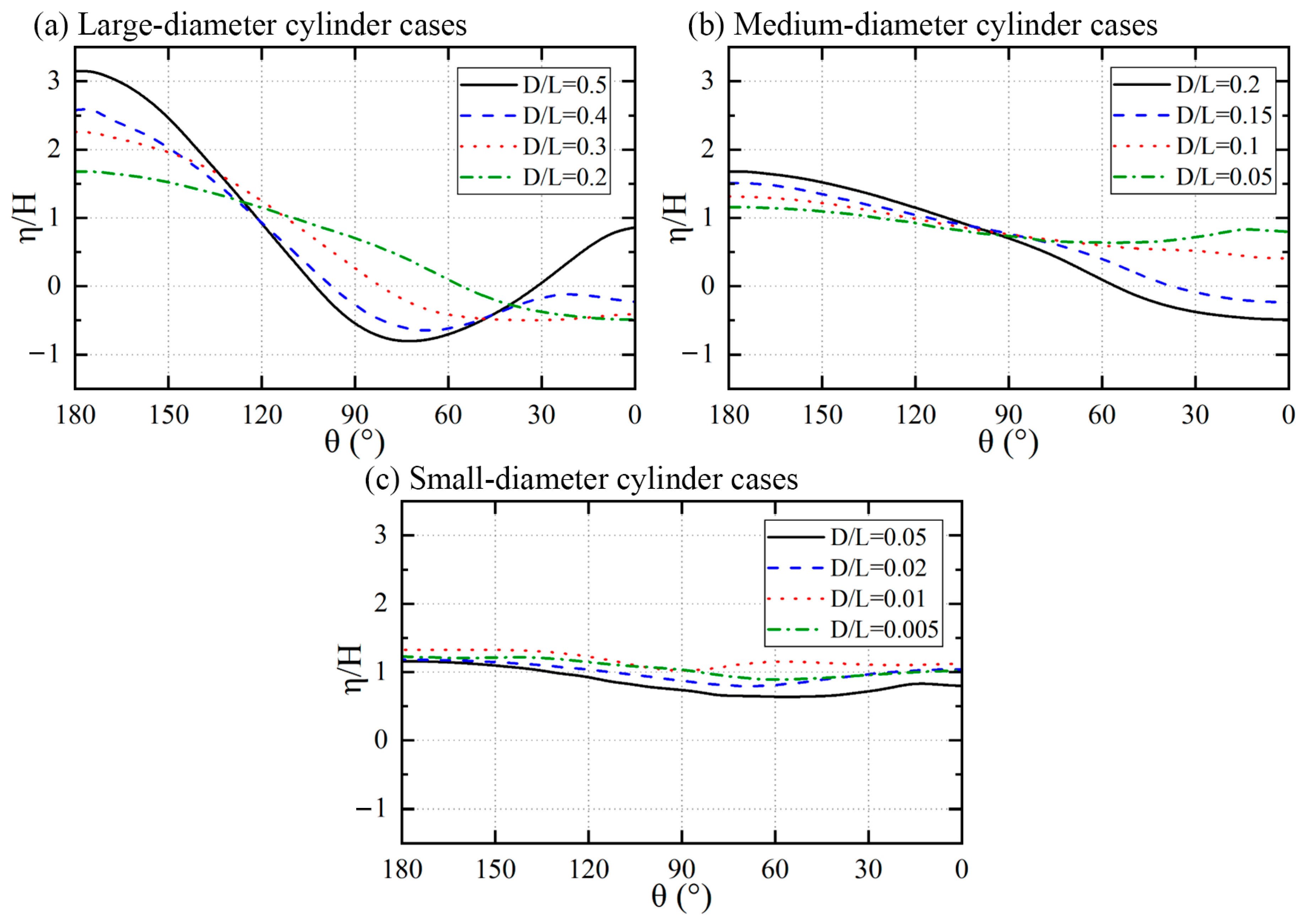
The maximum wave surging on the cylinder surface occurs at the apex of the wave-facing side of the cylinder. As shown in Figure 10, the wave heights around the cylinder under different cylinder diameter cases at the moment of maximum surging are presented. In the large-diameter cylinder case shown in Figure 10a, as the cylinder diameter increases, the wave height distributions near both the wave-facing and leeward sides gradually increase. When $D/L=0.5$, a remarkably distinct minimum wave height appears near $\theta =73°$ at the rear side of the tail. As the cylinder diameter decreases, this minimum value gradually increases and shifts backward toward the leeward side. In the medium-diameter cylinder case (transition range from small to large diameters) shown in Figure 10b, as the cylinder diameter increases, the wave height amplitude near the wave-facing side gradually increases, while the wave height near the leeward side gradually decreases. When $D/L=0.1$, the wave height distributions around the circumference tend to be uniform. Within the transition range, the minimum wave height only appears on the leeward side of the cylinder. For the small-diameter cylinder with $D/L=0.05$, the minimum value shifts forward again. In the small-diameter cylinder case shown in Figure 10c, as the cylinder diameter increases, the wave heights around the entire cylinder gradually decrease, and the minimum wave height reappears within the range of $\theta =70°~85°$.

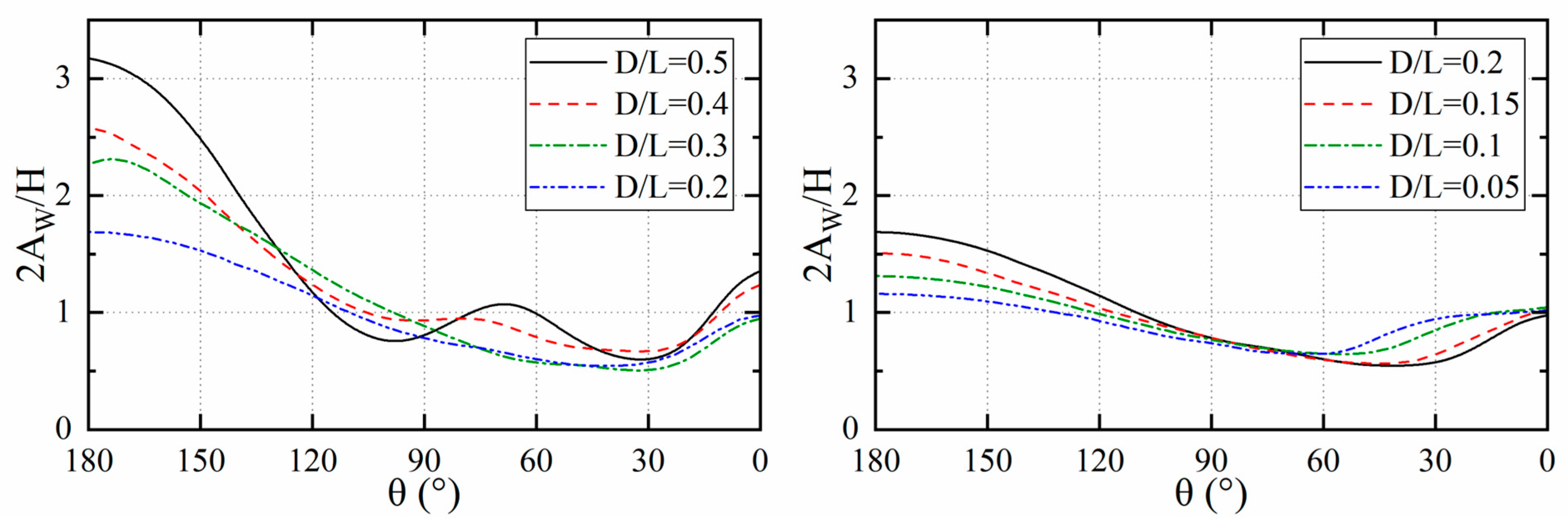
The wave amplitude $A_W$ extracted from each measurement point around the cylinder is nondimensionalized with the incident wave amplitude $H/2$, yielding the distribution of wave run-up ratio $2A_W/H$ around the cylinder under different cylinder diameter cases, as shown in Figure 11. In Figure 11, it can be seen that when the cylinder scale ranges from $D/L=0.2$ to $D/L=0.05$, the wave run-up distribution along the column is basically consistent. The maximum wave run-up occurs at the central position of the wave-facing side of the cylinder, after which the run-up amplitude gradually decreases due to continuous dissipation of water energy, reaching a minimum near $\theta =30°~60°$. Finally, two lateral waves propagating along the column sides superimpose near the leeward side of the column, causing an increasing trend in wave run-up amplitude. Different from the above patterns, starting from $D/L=0.2$, as the cylinder diameter increases, the diffraction effects on the wave field cause a secondary upward trend in waves within the $\theta =50°~80°$ range at the rear side of the cylinder, resulting in three maximum points at the wave-facing side, leeward side, and the rear side of the cylinder.

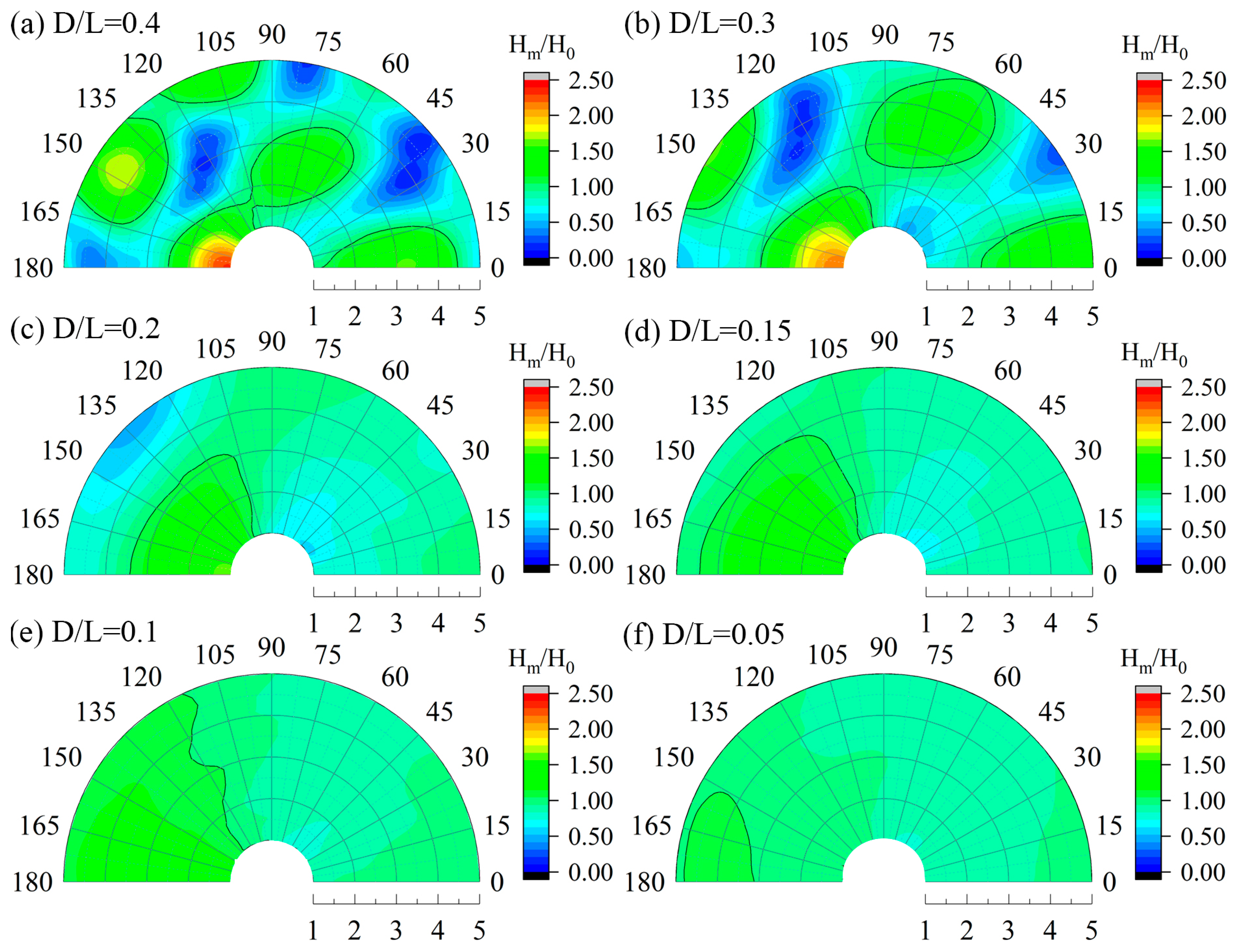
To demonstrate the diffraction effect of the cylinder on the surrounding wave field, the average wave height $H_m$ at measurement points within $X/R=5$ around the cylinder is extracted in polar coordinates and compared with the incident wave height $H_0$, yielding the polar coordinate contour plot shown in Figure 12. The black solid line in the figure represents the $H_m/H_0=1$ contour line, and the wave direction is from left to right. As can be seen from the figure, from the wave-facing side at $\theta =180°$ to the leeward side at $\theta =0°$, regardless of the cylinder size, a wave trough always exists in the shadow zone between $\theta =30°~90°$ (the blue area at the rear side of the cylinder in the figure). As the cylinder diameter increases, the diffraction effect caused by the cylinder gradually intensifies, leading to a gradual reduction in the scope of high-wave and low-wave regions, with significant changes in the magnitude of average wave height and more concentrated energy. When $D/L=0.15$, the $H_m/H_0=1$ contour line is located within a 4-fold radius range. For $D/L=0.15$, the influence range of the $H_m/H_0=1$ contour line extends beyond 5 times the cylinder radius, and the variation amplitude of the average wave height within the 5-fold radius range has decreased to less than 15%, which can be approximately considered as having no influence on the surrounding wave field. The Morison equation is applied to solve the hydrodynamic coefficients.

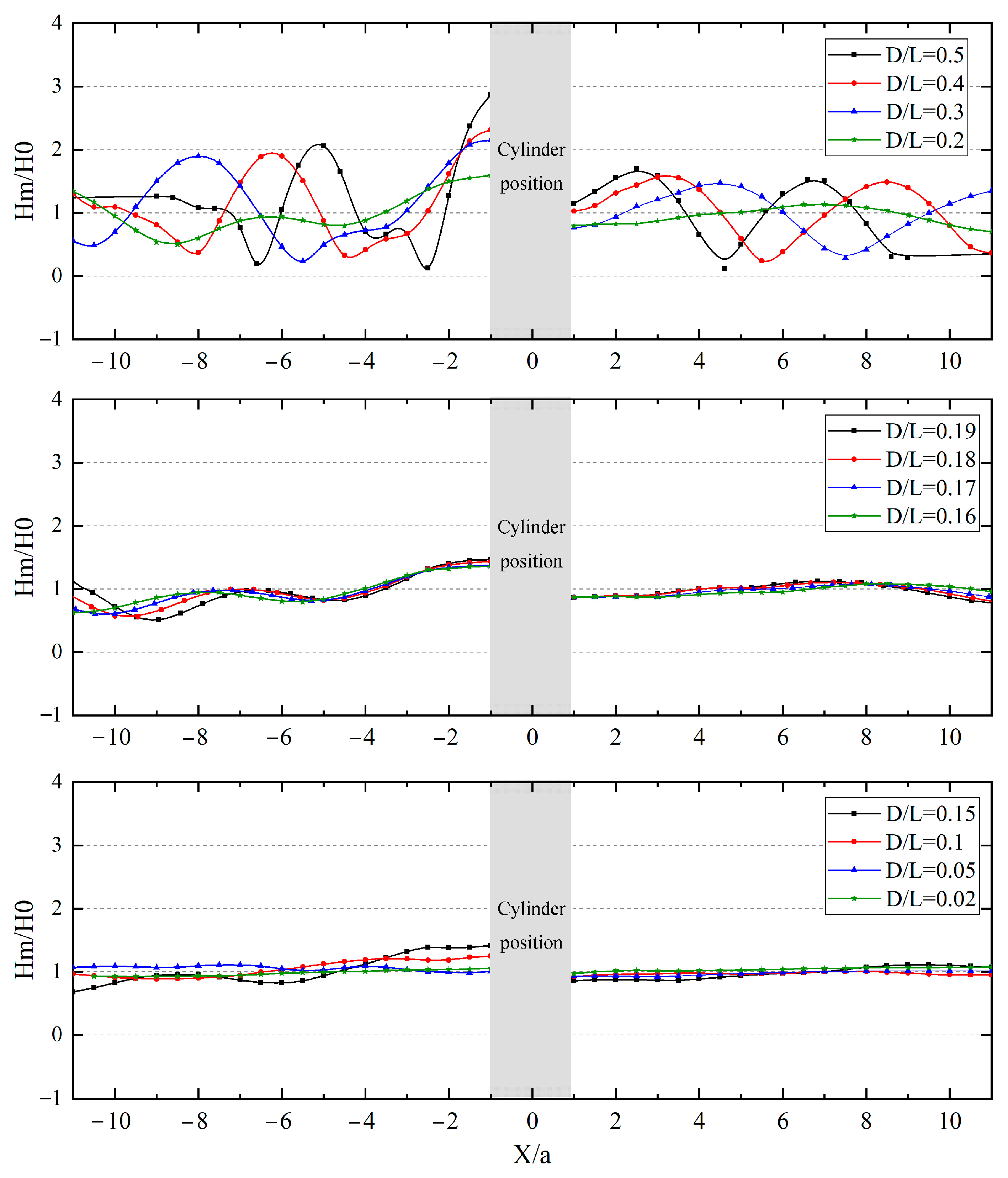
In studies on the wave dissipation effect of breakwaters, wave reflection and transmission coefficients are often used to evaluate the performance of breakwaters in dissipating waves. Regarding the influence of the cylinder on the surrounding wave field in this thesis, the reflection coefficient and transmission coefficient are similarly introduced to reflect the impact of the cylinder’s presence on the wave field generated by the superposition of front–back reflected waves and diffracted waves. The reflection coefficient $Kr$ is defined as the ratio of the average wave height at the measurement point of $\theta =180°$ to the incident wave height, and the transmission coefficient $Kt$ is defined as the ratio of the wave height at the measurement point of $\theta =0°$ to the incident wave height.

As shown in Figure 13, the variation laws of $Kr$ and $Kt$ with $D/L$ at different positions on the wave-facing and leeward sides of the cylinder under wave conditions of water depth $h=0.6 \mathrm{m}$ and wave height $H=0.06 \mathrm{m}$ are presented. To facilitate the display and comparison of coefficient changes in the front and rear regions, this series of cases is divided into large-diameter cylinder cases, transition–range–diameter cylinder cases, and small-diameter cylinder cases. The gray area in the middle represents the actual position of the cylinder. The abscissa denotes the ratio of the distance from the linear measurement points at $\theta =180°$ and $\theta =0°$ to the cylinder’s center to the radius. The left side of the cylinder is the wave incoming direction, meaning the left curve represents the reflection coefficient curve at $\theta =180°$, and the right curve represents the transmission coefficient curve at $\theta =0°$.

As can be seen from the reflection coefficient curve on the left side of the cylinder position, the presence of the cylindrical structure has a significant impact on the wave fields in the front and rear regions, and this impact gradually intensifies as the cylinder diameter increases. The extreme values in both the reflection coefficient and transmission coefficient curves reach larger or smaller magnitudes as the cylinder diameter increases. Overall, in terms of horizontal coordinate positions, increasing the cylinder diameter produces a very obvious compressing effect on the reflection and transmission coefficients of the surrounding wave field, indicating that the diffraction effect caused by the larger cylinder diameter gradually strengthens. Conversely, as the cylinder diameter decreases, the coefficients at each point gradually tend toward 1. In terms of the reflection coefficient, when $D/L=0.2$, there is still a significant impact on the reflection coefficients between $X/R=1~2.5$ and $X/R=7.5~9.5$. When $D/L=0.15$, only the influence of wave reflection near the cylinder within $X/R=1~3$ needs to be considered. For the transmission coefficient, when $D/L<0.2$, the influence of cylinder scale on wave transmission within $X/R=1~5$ can be disregarded; when $D/L<0.15$, the influence of cylinder scale on wave transmission within $X/R=1~10$ no longer needs to be considered.

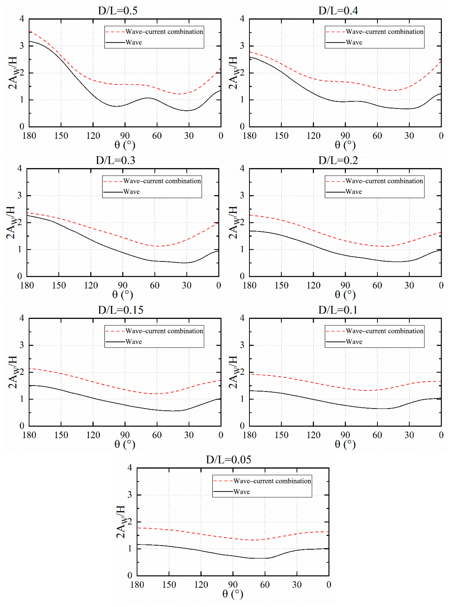
4.2. Wave Climb Under Combined Wave–Current Condition

To study the influence of water flow on wave run-up around the cylinder, a water flow with u = 0.1 m/s is added under wave conditions, and the resulting wave run-up distribution is shown in Figure 14. As shown in the figure, the presence of current significantly enhances the wave run-up effect across all cases. The distribution curves of wave run-up for each group of D/L cylinders under wave–current conditions exhibit trends similar to those under pure wave conditions. However, the influence of current on wave run-up around cylinders is not a simple linear amplification: the wave run-up near the wave-facing side is consistently smaller than that near the wave-back side. With the decrease in D/L, the wave run-up near the wave-facing side gradually approaches that near the wave-back side. Additionally, it is likely that due to the increase in cylinder size, the diffraction effect under current becomes more pronounced, leading to a stronger superposition effect of edge waves propagating from both sides near the wave-back side of the cylinder.

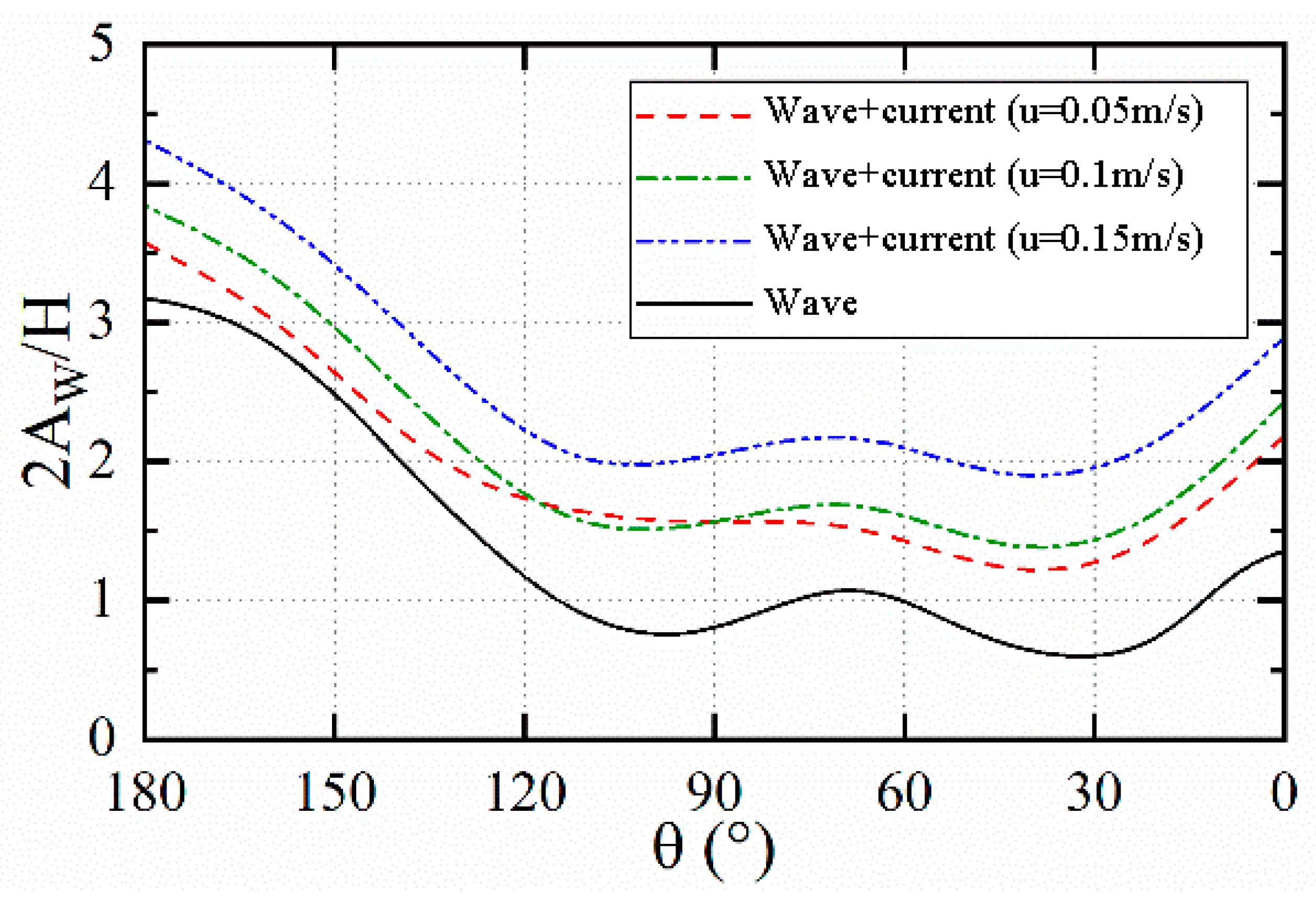
To investigate the influence of water flows with different velocities on the wave field, different flow velocities were added under the same wave field conditions. The wave height time history curves at the wave-facing side measurement points and the surrounding wave run-up distributions for the cylinder case with $D/L=0.5$ are shown in Figure 15. As can be seen from the figure, under the co-directional action of waves and currents, when the incident wave parameters and cylinder diameter remain unchanged, the greater the water flow velocity, the larger the overall upward displacement of the wave surface, and the more pronounced the wave run-up effect. The wave run-up on the wave-facing side of the cylinder exhibits linear growth: under pure waves, $2A_W/H$; at u = 0.05 m/s, $2A_W/H$ reaches 3.58; at u = 0.1 m/s, it reaches 3.84; and at u = 0.15 m/s, it reaches 4.31. The wave run-up on the leeward side increases significantly at u = 0.05 m/s. Although the incident wave amplitude near $\theta =90°~120°$ increases slightly at u = 0.05 m/s, possibly due to numerical simulation residual accumulation, the increase in wave run-up height under wave–current combined conditions is very evident. This is because the increase in water particle velocity raises the fluid kinetic energy in the waves. This increase in kinetic energy directly reflects the enhancement of wave energy, enabling more energy to be released during wave–cylinder interaction. Part of the kinetic energy is converted into potential energy, causing run-up on the column surface with increased height, thereby increasing potential energy. This energy conversion process is an intuitive manifestation of the law of conservation and transformation of energy.

4.3. Mechanical Characteristics of Fan Foundation

For the regular waves involved in this paper, the maximum horizontal wave force F on the cylinder over the entire wave period can be regarded as a function of the following dimensional parameters: diameter $D$, wavelength $L$, wave height $H$, water depth $h$, density $\rho$, gravitational acceleration $g$, and kinematic viscosity $\nu$. Taking $\rho$, $g$, and $\nu$ as fundamental parameters, it can be obtained that

$${\displaystyle \frac{F}{\rho gA{D}^2}}=f\left({\displaystyle \frac{D}{L}},{\displaystyle \frac{H}{L}},{\displaystyle \frac{h}{L}},{\displaystyle \frac{\nu }{\sqrt{g{L}^3}}}\right)=f\left({\displaystyle \frac{D}{L}},kA,kh,\mathrm{Re}\right)$$

(32)

where $k$ is the wave number, ${\displaystyle \frac{D}{L}}$ is the cylinder scale, $kA$ is the nondimensional wave amplitude, $kh$ is the nondimensional water depth, and Re is the Reynolds number.

Based on the above dimensional analysis, three groups of cases under different conditions were set up to study the characteristics of wave forces on wind turbine foundations within common scale ranges. Group A cases focus on the force characteristics of cylinders in the transition interval of cylinder scale $D/L$ from 0.1 to 0.2, with a total of 18 cases, including 9 deep-water conditions (marked with ○) and 9 finite water depth conditions (marked with △). The wave parameters are set as shown in

Table 4. Group A operating conditions.

Case	D/L	kA	kh	Re	KC	Deep-Water Conditions
A1	0.1	0.105	2.0933	66,914	1.05	△
A2	0.1	0.157	2.0933	100,372	1.57	△
A3	0.1	0.209	2.0933	133,829	2.09	△
A4	0.15	0.105	2.0933	100,372	0.70	△
A5	0.15	0.157	2.0933	150,557	1.05	△
A6	0.15	0.209	2.0933	200,743	1.40	△
A7	0.2	0.105	2.0933	133,829	0.52	△
A8	0.2	0.157	2.0933	200,743	0.79	△
A9	0.2	0.209	2.0933	267,657	1.05	△
A10	0.1	0.161	4.1866	101,886	1.57	○
A11	0.1	0.215	4.1866	135,847	2.09	○
A12	0.1	0.269	4.1866	169,809	2.62	○
A13	0.15	0.161	4.1866	152,828	1.05	○
A14	0.15	0.215	4.1866	203,771	1.40	○
A15	0.15	0.269	4.1866	254,714	1.74	○
A16	0.2	0.161	4.1866	203,771	0.79	○
A17	0.2	0.215	4.1866	271,695	1.05	○
A18	0.2	0.269	4.1866	339,619	1.31	○

.

The Group B cases are the same as those used in Section 4.1. Under the same wave field conditions, by changing the cylinder diameter, the force characteristics of cylindrical foundations with different diameters in the same wave field are obtained. The Group C cases refer to the wave parameters and water depth conditions of the sea area where the first-phase project of the Nanri Island Offshore Wind Farm in Putian, Fujian is located. Taking a cylinder diameter $D=12 \mathrm{m}$ and water depth $h=60 \mathrm{m}$, the period T uniformly transitions in the range of 2.5~13.5 s, the wave height ranges from 0.5 m to the maximum design wave height (taking the wave height with a cumulative frequency of $H_{1\%}$), and the range of $D/L$ is in the range of 0.047~0.63. The specific parameters are shown in Figure 16.

This study focuses on the variation laws of horizontal wave forces within the range of $0.1\le D/L\le 0.2$ under different water depths and wave heights. This not only helps better understand and predict the changes in wave forces within this range but also provides an important reference for the design of offshore wind turbine foundation structures and pile structures.

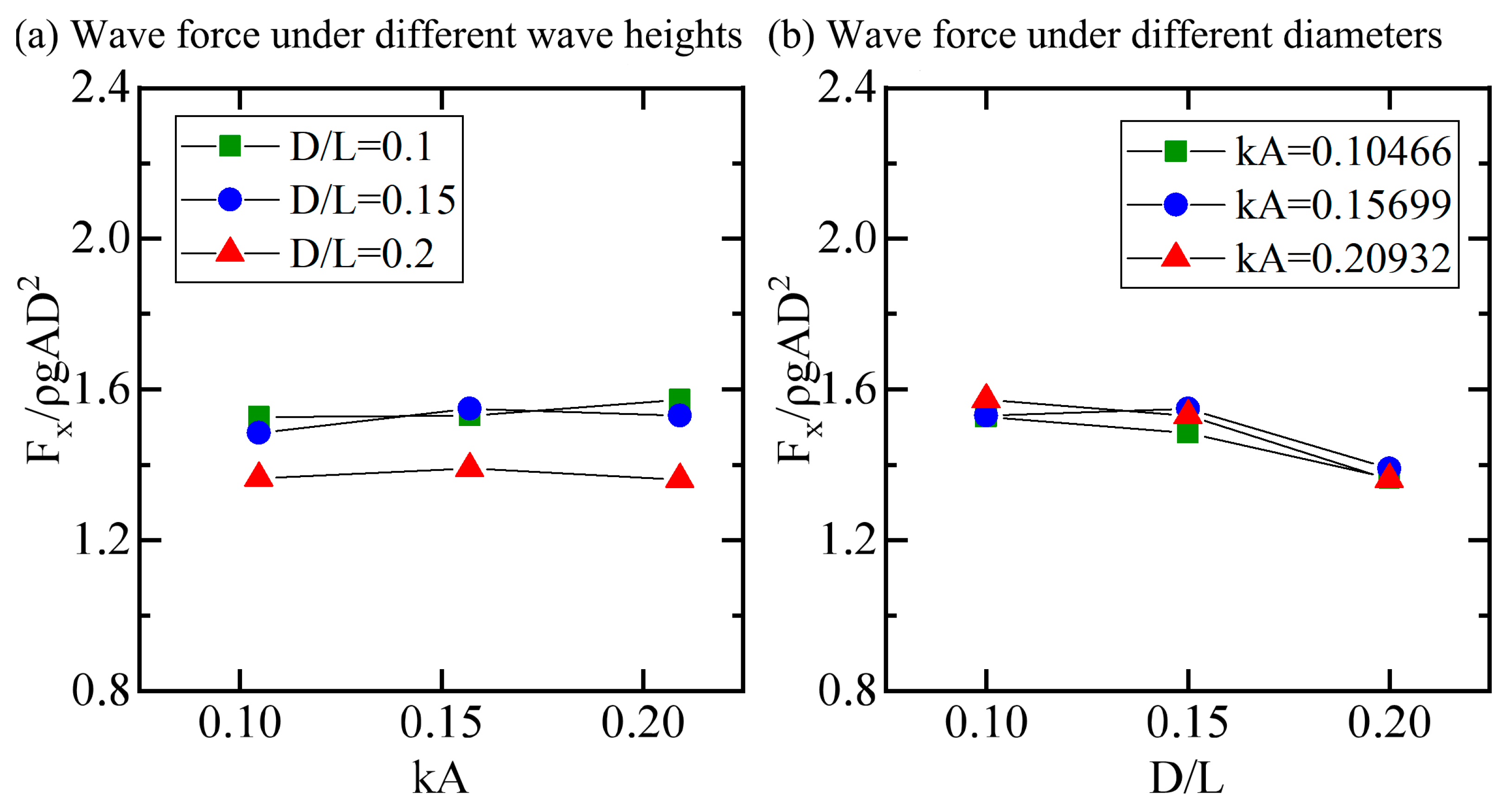
The calculation results of horizontal along-current wave forces are nondimensionalized, and the results for each case under finite water depth conditions are shown in Figure 17a, which presents the force results on the cylinder under different wave heights. It can be seen that as the nondimensional wave amplitude increases, the nondimensional horizontal wave forces at $D/L=0.1$ and $D/L=0.15$ show a slow increasing trend. At $D/L=0.2$, the nondimensional horizontal wave force on the cylinder is the smallest. Figure 17b shows the variation in horizontal wave forces on cylinders with different diameters. As the cylinder diameter increases, the nondimensional horizontal wave force gradually decreases, and the wave height conditions have little influence on the nondimensional horizontal wave force.

As shown in Figure 18, the calculation results of nondimensional wave forces under deep-water conditions for different wave heights and cylinder diameters are presented. Overall, compared with the finite water depth cases, the overall variation trends of the two are basically consistent. In Figure 18a, as the nondimensional wave amplitude increases, $D/L=0.1$ and $D/L=0.2$ always exhibit an upward trend. Only at $D/L=0.15$ does the nondimensional wave force show a downward trend. In Figure 18b, compared with the horizontal wave forces under finite water depth conditions, the influence of wave height on the nondimensional wave force is most significant at $D/L=0.1$.

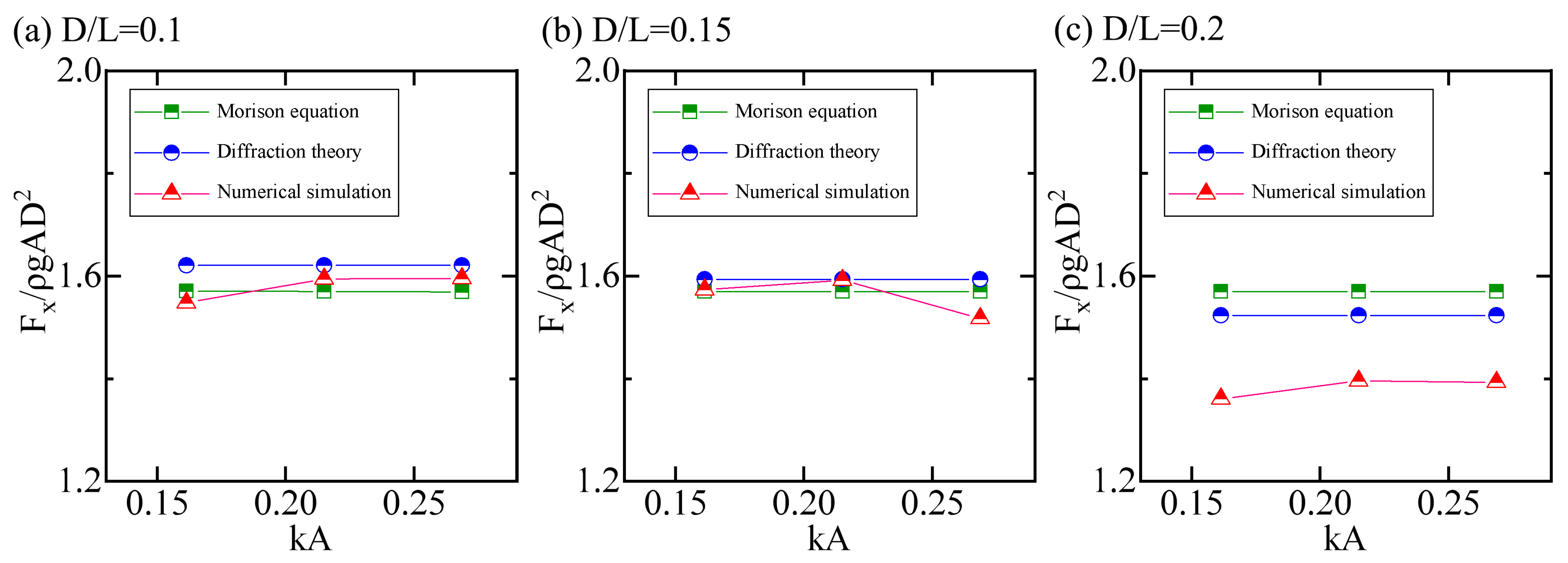
To further investigate the differences between the numerical simulation results and the results calculated by empirical formulas in engineering codes, two methods were employed: Morison’s equation for calculating wave forces on small-diameter cylinders and the diffraction theory for large-diameter cylinders. Detailed calculations of horizontal wave forces on vertical cylinders were conducted for these cases using both methods. The maximum horizontal wave forces obtained from Morison’s equation, linear diffraction theory in codes, and numerical simulations were compared to analyze the differences among the three sets of results. The comparisons of horizontal wave forces under finite water depth and deep-water conditions are shown in Figure 19 and Figure 20, respectively.

As can be seen from Figure 19 and Figure 20, the results from Morison’s equation and diffraction theory do not change with $kA$. The wave forces calculated using Morison’s equation hardly change with the cylinder diameter, while the maximum wave forces calculated using diffraction theory gradually decrease as the cylinder diameter increases. However, comparisons with numerical simulation results show that the results from Morison’s equation and diffraction theory are only accurate when $D/L=0.1$ and $D/L=0.15$. Morison’s equation provides more accurate estimates at $D/L=0.1$, and there is little difference between the two wave force estimation methods at $D/L=0.15$, with errors within 5%. Only slight deviations in the nondimensionalized maximum wave force occur due to changes in wave height. However, serious deviations occur when $D/L=0.2$, where both empirical formulas overestimate the horizontal wave forces by more than 10%, indicating that using Morison’s equation to calculate wave loads is no longer applicable. This may be due to the disturbance caused by the cylinder in the wave field, which reduces the nondimensional inertial force on the cylinder. Therefore, it is necessary to modify the diffraction theory.

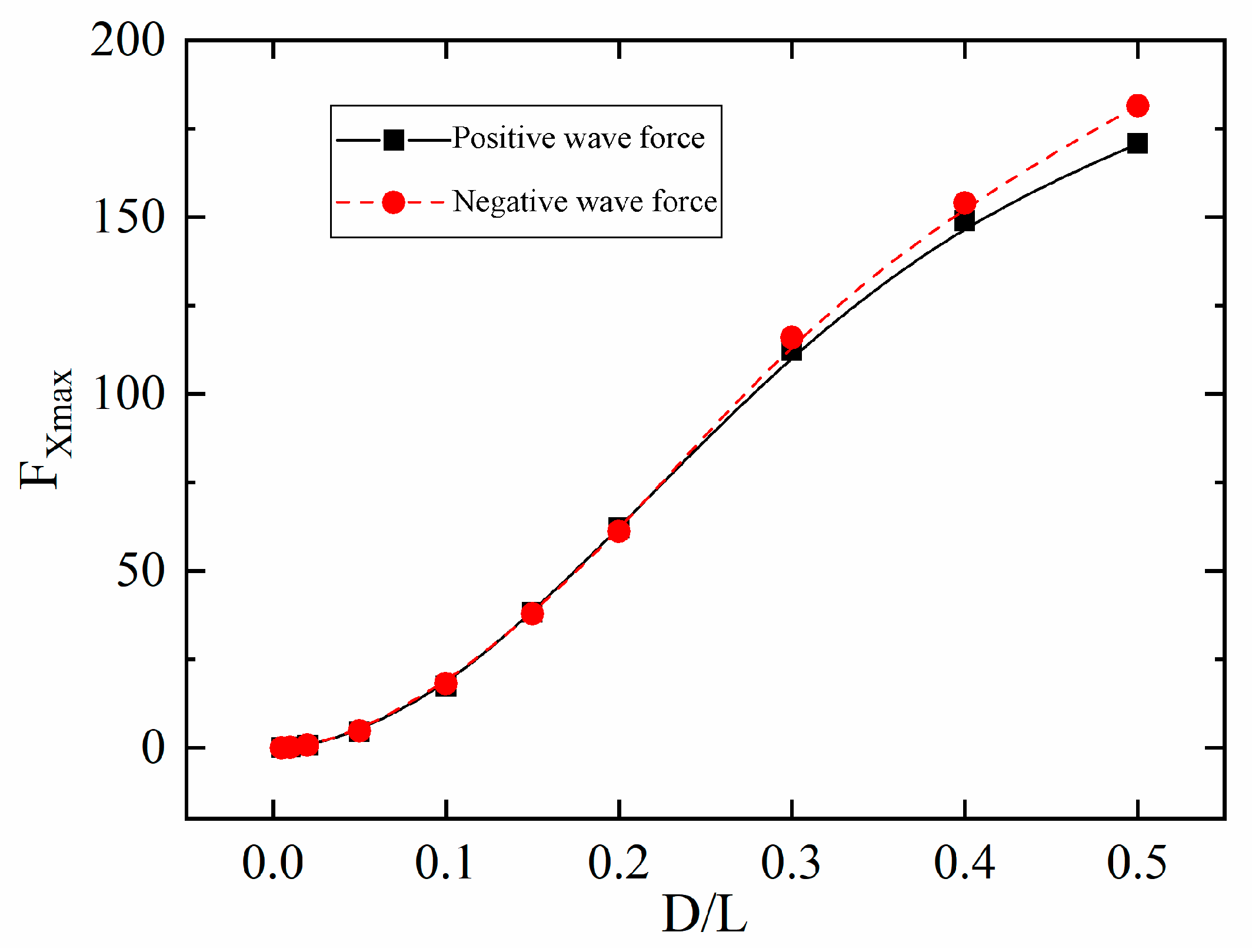
In wave motion, due to the reciprocating motion of water particles in the flow, the wave forces on the cylindrical structure are also reciprocating, i.e., positive and negative. The force exerted by waves on structures in the same direction as wave propagation is defined as the positive wave force, occurring when water particle motion aligns with the wave propagation direction. After wave passage, water retreat or the formation of a low-pressure zone behind the structure causes water particles to move opposite to the wave propagation direction, whereby the force exerted by waves on the structure in the opposite direction to wave propagation is termed the negative wave force. As shown in Figure 21, the curves depict the variation in the maximum positive and negative horizontal wave forces on the cylindrical structure with the cylinder scale. It can be seen that the maximum positive and negative horizontal wave forces on the cylindrical structure exhibit basically the same trend. Except for $D/L=0.15$ and $D/L=0.2$, the negative horizontal wave forces are slightly higher than the positive ones, with a difference of 4–5%, which may be caused by the nonlinear effects of waves. At the boundary point of cylinder size between $D/L=0.1$ and $D/L=0.2$, the growth rate of horizontal wave forces on the cylinder significantly accelerates, which is basically consistent with the results derived from linear diffraction theory.

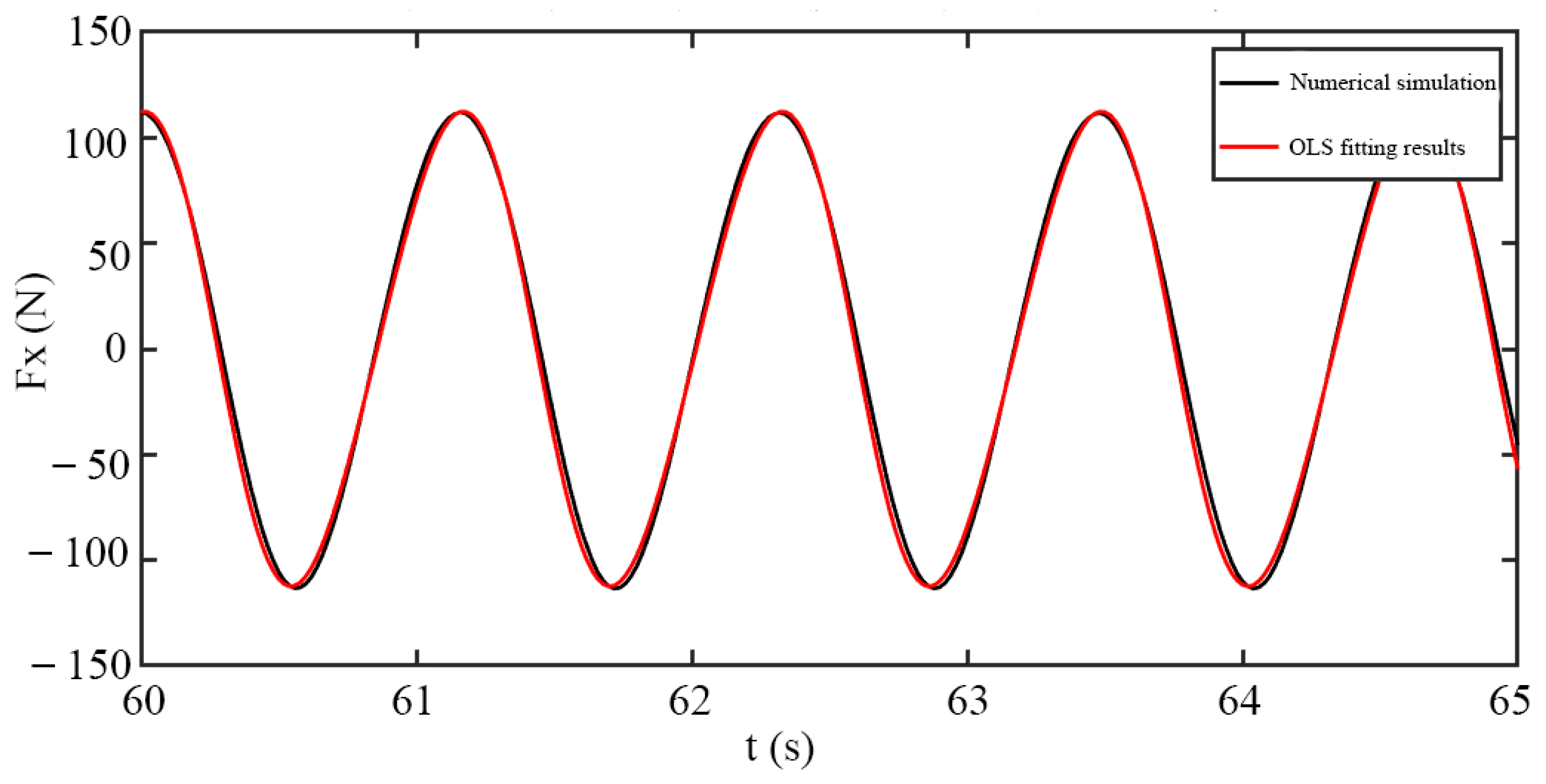
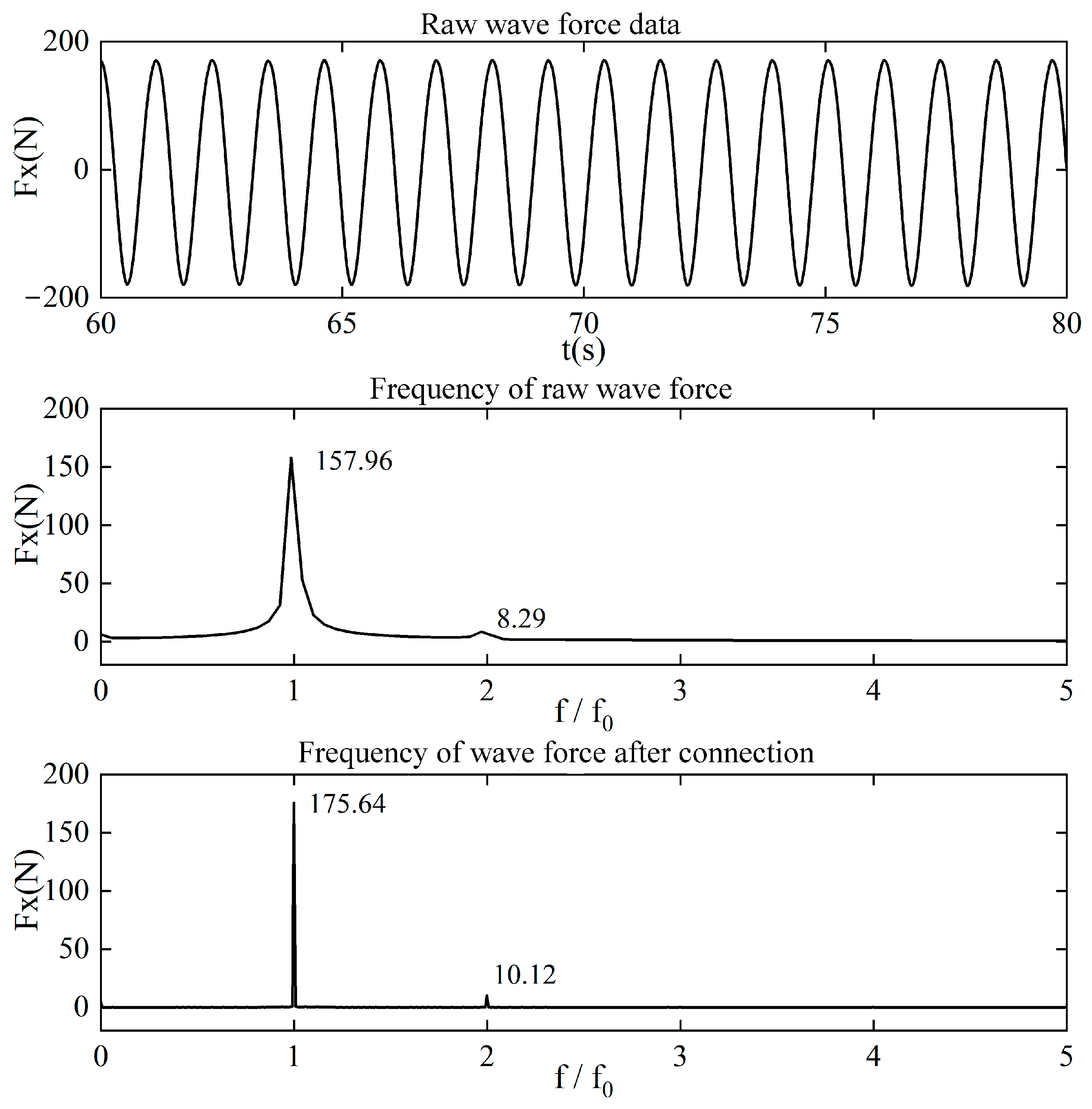
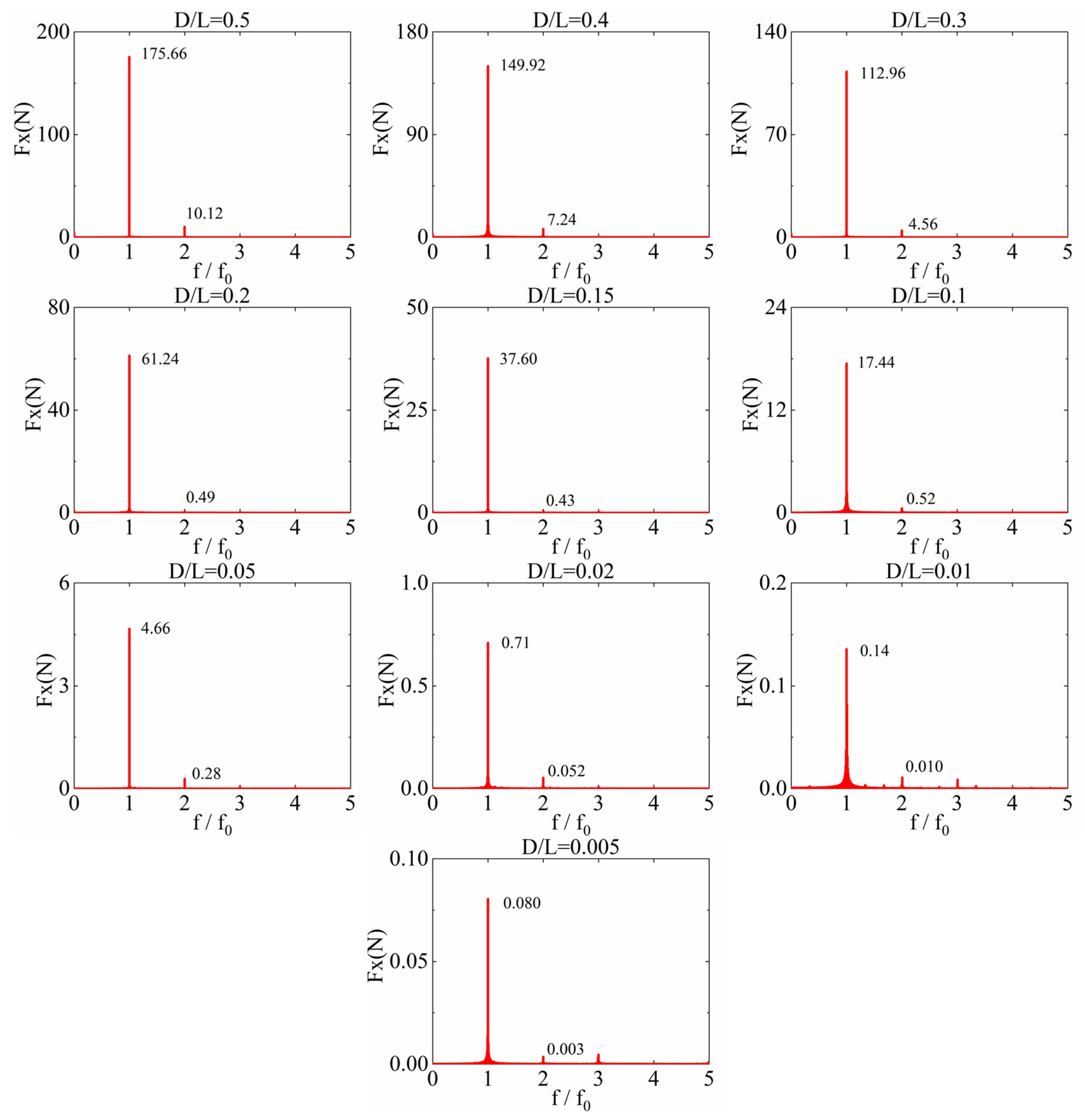
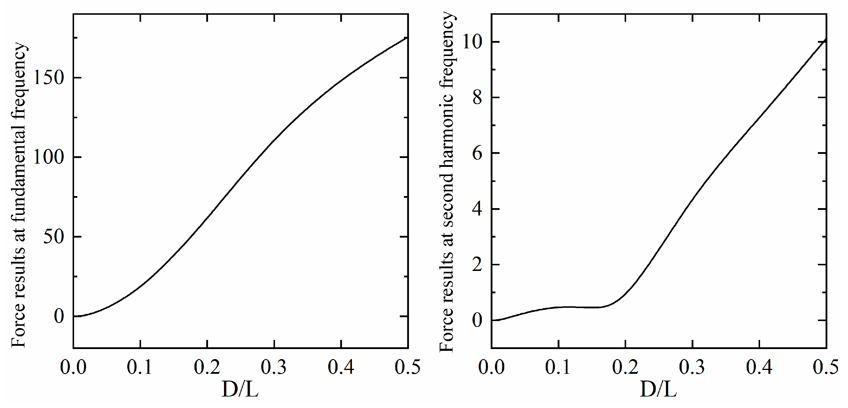
By concatenating 12 stable periods for each case and performing FFT (Fast Fourier Transform) analysis, the frequencies and amplitudes of each order of forces on cylindrical structures with different diameters are obtained. After filtering the first and second harmonic forces for each case, the force distributions at different frequencies for cylindrical structures of various scales are shown in Figure 22. As can be seen from the figure, as the cylinder diameter increases, the forces at both the first and second harmonic frequencies gradually increase.

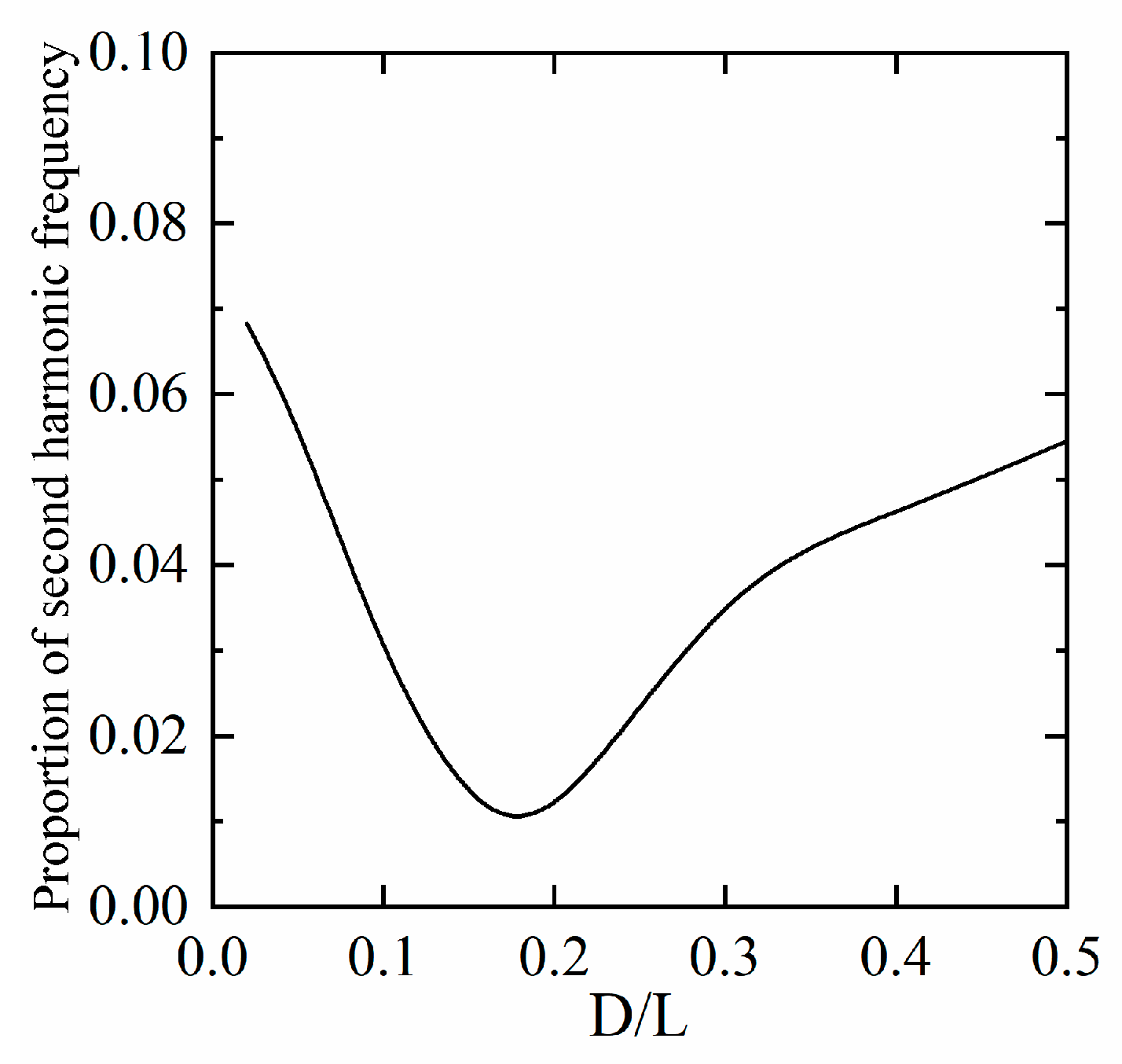
Figure 23 and Figure 24 show the variation curve of the proportion of the second harmonic force on the wind turbine foundation with the cylinder scale. As can be seen from the figure, as the cylinder scale increases, the horizontal wave force at the second harmonic frequency on the structure exhibits a horizontal phase in the transition region between 0.1 and 0.2, indicating that within this transition region, the nonlinear effects of the horizontal wave loads on the wind turbine foundation remain constant as the cylinder scale increases. The proportion of nonlinear horizontal wave loads is minimized near $D/L=0.2$.

In large-diameter cases, the inertial force coefficient dominates the influence on wave forces, while nonlinear effects enhance the diffraction effect. The $C_M$ value obtained by fitting with diffraction theory using the least squares method is more accurate than that from Morison’s equation using the same fitting method. As shown in Figure 25, the $C_M$ results are obtained by fitting wave forces on cylinders of different diameters with Morison’s equation for $D/L\le 0.1$ and with linear diffraction theory for $D/L>0.1$. It can be seen from the figure that as the cylinder diameter increases, the inertial force coefficient $C_M$ gradually decreases, showing some similarity to the $C_M$ values given by linear diffraction theory. When $D/L<0.05$, fitting cylinder wave forces with Morison’s equation using the least squares method yields a viscous force coefficient $C_D$ of approximately 1.35. During the fitting process with Morison’s equation, it is found that for $D/L\ge 0.05$, the value of the viscous force coefficient $C_D$ has little effect on wave forces, with only $C_M$ playing a role in the fitting. This indicates that within the range of $D/L\ge 0.05$, the viscous forces generated by waves are very small and their proportion in the total force can be ignored. According to Sarpkaya’s [19] recommendation, $C_D=0.62$ is used for calculations.

4.4. Force Characteristics of Cylinder Under Real Sea Conditions

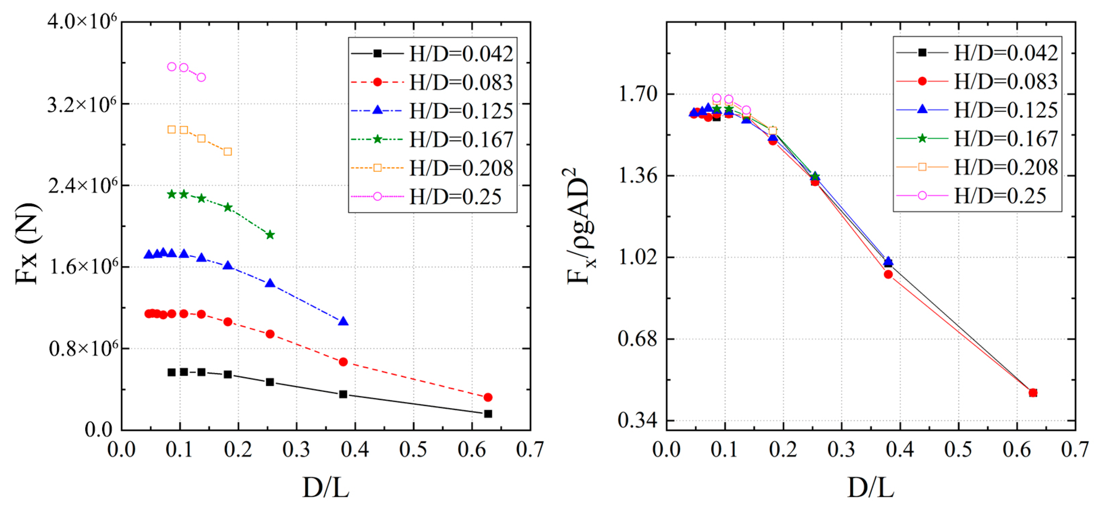
In the Group C experimental cases, referring to the wave parameters and water depth conditions of the sea area where the first-phase project of the Nanri Island Offshore Wind Farm in Putian, Fujian is located, the maximum horizontal wave force on a wind turbine foundation with a diameter $D=12 \mathrm{m}$ in the wave field under the set wave conditions is shown in Figure 26. As can be seen from the figure, under the same wave height condition, as the wavelength increases, the horizontal wave load on the structure slowly increases. When $D/L<0.1$, the variation range of the maximum horizontal wave force on the wind turbine foundation is small and basically remains stable. It can be seen from the left figure that the wave height H is a key factor affecting the maximum horizontal wave force on the wind turbine foundation. The right figure shows the result of nondimensionalizing the maximum horizontal wave force, from which it can be seen that the variation trend of the nondimensionalized wave force remains basically consistent. The maximum wave force increases rapidly with the wave height, and this is more evident at larger wavelengths, indicating that the inertial force generated by waves increases with the wave height.

As shown in Figure 27, the variation law of the inertial force coefficient $C_M$ with $D/L$ under different wave heights is presented. The $C_M$ results are also obtained by fitting wave forces with Morison’s equation for $D/L\le 0.1$ and with linear diffraction theory for $D/L>0.1$.

During the fitting process using Morison’s equation, the viscous force component of the wave is similarly found to be very small. Therefore, it is also recommended to use $C_D=0.62$ for calculations in engineering applications. Additionally, it can be seen from the figure that when $D/L>0.2$, the numerical values and variation patterns of $C_M$ basically tend to be consistent. When $D/L<0.2$, as $D/L$ decreases, the influence of wave height on the value of $C_M$ gradually increases. In this interval, the diffraction effect gradually weakens, and inertial forces dominate.

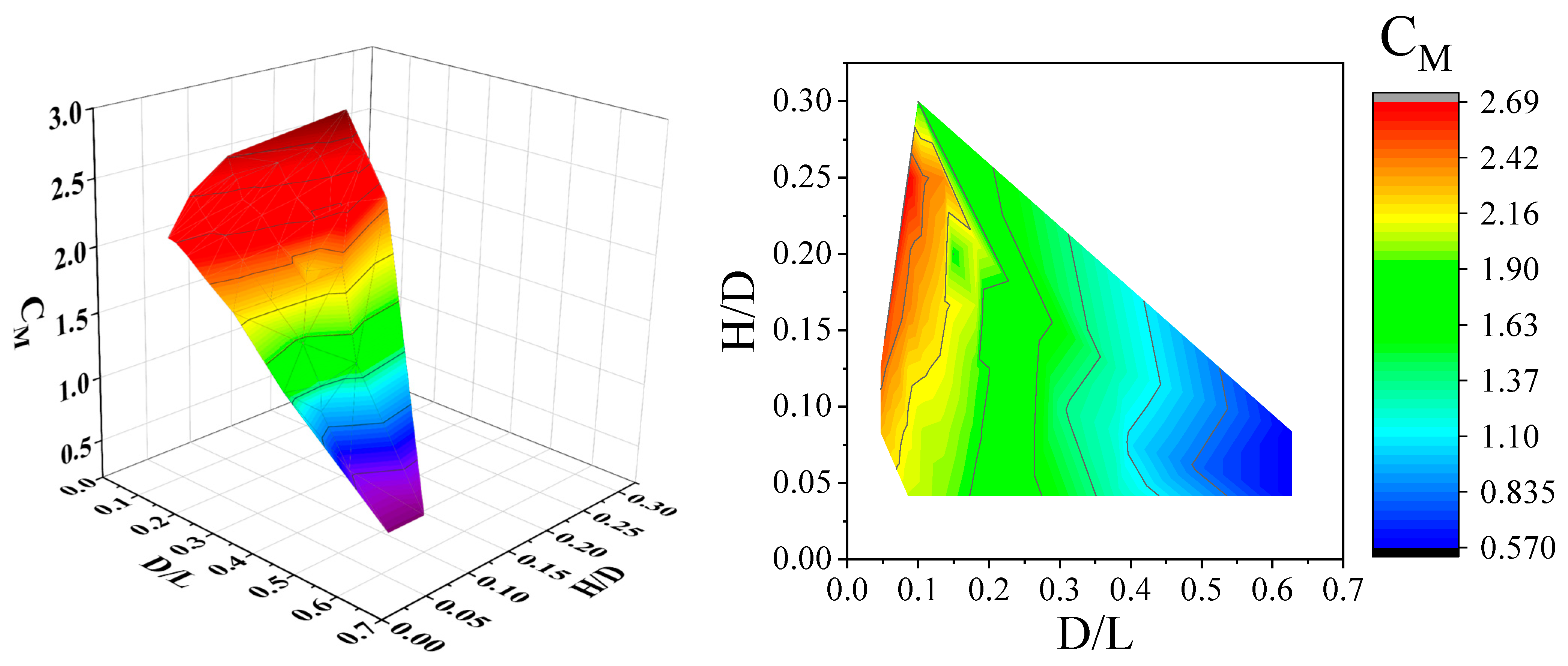
To simplify the calculation process, empirical formulas hold an important position in engineering calculations. Equation (33) defines the boundary between large-diameter and small-diameter cylinders as 0.1 by organizing hydrodynamic coefficients, and the values of $C_D$ and $C_M$ are redefined using wave forces obtained from numerical simulations and applied as a revised formula. Here, the value of $C_D$ is taken as 0.62, and the recommended value of $C_M$ is shown in Figure 28.

$$F_x=\left\{\begin{array}{ccc}{C}_M{\displaystyle \frac{\gamma AH}{2}}{K}_2& ,& D/L>0.1\\ C_D{\displaystyle \frac{\gamma D{H}^2}{2}}{K}_{1}cos\omega t\left|cos\omega t\right|-C_M{\displaystyle \frac{\gamma AH}{2}}{K}_{2}sin\omega t& ,& D/L\le 0.1\end{array}\right.$$

(33)

where $K_1={\displaystyle \frac{\frac{4\pi z_2}{L}-\frac{4\pi z_1}{L}+\mathit{sinh}\frac{4\pi z_2}{L}-\mathit{sinh}\frac{4\pi z_1}{L}}{8\mathit{sinh}\frac{4\pi h}{L}}}$, $K_2={\displaystyle \frac{\mathit{sin}h\frac{2\pi z_2}{L}-\mathit{sin}h\frac{2\pi z_l}{L}}{\mathit{cos}h\frac{2\pi h}{L}}}$

Figure 28 displays a recommended value contour plot of the wave inertial force coefficient $C_M$ based on Morison’s equation and linear diffraction theory, under the target water area conditions where the relative water depth $D/L$ ranges from 0.047 to 0.63 and the relative wave height $H/D$ ranges from 0.05 to 0.3. By referring to this figure and combining it with the differences in specific environmental parameters, the value of the coefficient $C_M$ can be determined more accurately.

5. Conclusions and Prospection

Regarding the variation in the wave field around the cylinder, the following conclusions can be drawn:

• Starting from $D/L=0.2$, as the cylinder diameter increases, the diffraction effect on the wave field causes a secondary upward trend in the wave at the rear side of the cylinder $\theta =50°~80°$, with three maximum points appearing at the wave-facing side, leeward side, and the rear side of the cylinder.
• When $D/L=0.15$, the contour line of $H_m/H_0=1$ is within a 4-fold radius range. For $D/L=0.15$, the influence range of the $H_m/H_0=1$ contour line extends beyond 5 times the cylinder radius, and the average wave height variation amplitude within the 5-fold radius range has decreased to less than 15%. It can be approximately considered that there is no influence on the surrounding wave field, and Morison’s equation is applied to solve the hydrodynamic coefficients.
• In terms of the reflection coefficient, when $D/L=0.2$, there is still a significant influence on the reflection coefficients between $X/R=1~2.5$ and $X/R=7.5~9.5$. When $D/L=0.15$, only the influence of wave reflection near the cylinder within $X/R=1~3$ needs to be considered. For the transmission coefficient, when $D/L<0.2$, the influence of cylinder scale on wave transmission within $X/R=1~5$ can be disregarded; when $D/L<0.15$, the influence of cylinder scale on wave transmission within $X/R=1~10$ no longer needs to be considered.

Regarding the force on the cylinder, the following conclusions can be drawn.

The force characteristics of cylindrical structures with different diameters under the same wave field conditions were studied, and it was found that the variation trends of the maximum wave force and phase delay are basically consistent with linear diffraction theory. The derivation results show that the wave force delay on the cylindrical structure is mainly determined by inertial force. The horizontal wave force at the second-order frequency on the structure exhibits a horizontal phase in the transition region in the range of 0.1~0.2, indicating that within this transition region, the nonlinear effects of the horizontal wave loads on the wind turbine foundation remain constant as the cylinder scale increases. Based on the wave parameters and water depth conditions of actual wind farms, the causes of changes in hydrodynamic load coefficients were analyzed, and a revised empirical formula was proposed.

In this study, the wave field around cylinders was observed to determine the influence domain of diffraction effects on the wave field by considering the impacts of parameters, including cylinder diameter, wave height, and flow velocity. Cylindrical structures with different diameters were then defined based on these findings. Further analysis was conducted on the hydrodynamic loading characteristics of cylindrical structures with varying diameters, addressing the issues in traditional theories regarding the boundary definition between large- and small-diameter cylinders and the applicability of nonlinear wave loads. Given the complex wave conditions in marine environments, where wave morphology and characteristics are constantly evolving, the nonlinear properties of waves become particularly pronounced. Under nonlinear conditions, the influence of waves on MC (Motion Compensation/Marine Craft, etc.) is more intricate, necessitating further research on how the degree of wave nonlinearity affects MC.