Article

Physics-Informed Deep Learning for Karst Spring Prediction: Integrating Variational Mode Decomposition and Long Short-Term Memory with Attention

by
Liangjie Zhao
1,*,
Stefano Fazi
2,
Song Luan
1,
Zhe Wang
1,
Cheng Li
1,
Yu Fan
1 and
Yang Yang
1,*
1
Institute of Karst Geology, Chinese Academy of Geological Sciences/Key Laboratory of Karst Dynamics, Ministry of Natural Resources & Guangxi Zhuang Autonomous Region/International Research Center on Karst under the Auspices of UNESCO, Guilin 541004, China
2
Water Research Institute (IRSA), National Research Council of Italy (CNR), 00015 Rome, Italy
*
Authors to whom correspondence should be addressed.
Water 2025, 17(14), 2043; https://doi.org/10.3390/w17142043
Submission received: 4 June 2025 / Revised: 1 July 2025 / Accepted: 3 July 2025 / Published: 8 July 2025

Abstract

Accurately forecasting karst spring discharge remains a significant challenge due to the inherent nonstationarity and multi-scale hydrological dynamics of karst hydrological systems. This study presents a physics-informed variational mode decomposition long short-term memory (VMD-LSTM) model, enhanced with an attention mechanism and Monte Carlo dropout for uncertainty quantification. Hourly discharge data (2013–2018) from the Zhaidi karst spring in southern China were decomposed using VMD to extract physically interpretable temporal modes. These decomposed modes, alongside precipitation data, were input into an attention-augmented LSTM incorporating physics-informed constraints. The model was rigorously evaluated against a baseline standalone LSTM using an 80% training, 15% validation, and 5% testing data partitioning strategy. The results demonstrate substantial improvements in prediction accuracy for the proposed framework compared to the standard LSTM model. Compared to the baseline LSTM, the RMSE during testing decreased dramatically from 0.726 to 0.220, and the NSE improved from 0.867 to 0.988. The performance gains were most significant during periods of rapid conduit flow (the peak RMSE decreased by 67%) and prolonged recession phases. Additionally, Monte Carlo dropout, using 100 stochastic realizations, effectively quantified predictive uncertainty, achieving over 96% coverage in the 95% confidence interval (CI). The developed framework provides robust, accurate, and reliable predictions under complex hydrological conditions, highlighting substantial potential for supporting karst groundwater resource management and enhancing flood early-warning capabilities.

1. Introduction

Karst aquifer systems are characterized by intricate multi-scale hydrological processes that challenge accurate prediction and sustainable management [1]. These aquifers exhibit complex interactions between conduit-dominated flow and diffuse fracture networks, resulting in highly nonlinear and nonstationary spring discharge behaviors [2,3]. Traditional process-based models require extensive hydrogeological knowledge and still struggle with complex karst conduits [4,5], while purely data-driven models can capture patterns but may violate physical laws [6]. This has motivated physics-informed machine learning approaches that integrate hydrodynamic processes or physical constraints into data-driven models [7,8].
Long short-term memory (LSTM) networks have become a fundamental tool in hydrological time-series forecasting over the past decade, with successful applications in groundwater and karst systems [9,10]. Their capacity to capture long-term dependencies and nonlinear relationships enables effective representation of memory effects commonly observed in aquifers and catchments [11,12]. In karst environments, where spring discharge often responds to precipitation with a delay and exhibits prolonged recession behavior, LSTM models have consistently outperformed traditional neural network architectures. Empirical studies have reported superior predictive performance of LSTM compared to conventional statistical models in replicating observed spring flow dynamics [13,14,15]. Several studies have explored the integration of physically based models with data-driven techniques to leverage their complementary strengths [16]. Liu coupled a conceptual hydrologic model with an LSTM network and reported substantial improvements in streamflow simulations compared to either component used independently. A similar approach was adopted by Wu [17], who embedded an LSTM-based water use module within a rainfall–runoff simulator, resulting in reduced prediction error and enhanced physical consistency. Such developments have been shown to improve the representation of both extreme flow events and recession dynamics [18] while also maintaining physical plausibility under extrapolation conditions.
In karst systems, spring discharge is governed by processes operating across distinct temporal scales, such as rapid conduit flow during storm events and delayed baseflow contributions from matrix and epikarst storage [19]. Recent studies have demonstrated the growing effectiveness of coupling variational mode decomposition (VMD) with LSTM networks for forecasting highly nonlinear and nonstationary hydrological systems, particularly karst spring discharge [20,21]. The commonly adopted modeling framework employs a decompose–predict–reconstruct approach wherein VMD is first used to partition the discharge time series into a finite set of band-limited intrinsic mode functions (BLIMFs), each representing a specific frequency component [22,23]. These components are subsequently modeled using individual LSTM sub-networks, and the final discharge prediction is obtained through recombination of the forecasted components [24]. For instance, An [25] assessed the performance of SSA-LSTM, EEMD-LSTM, and a standard LSTM model using data from the Niangziguan karst spring and reported superior accuracy for the EEMD-LSTM configuration due to its enhanced tolerance to noise. Building on these findings, Wang [26] incorporated an attention mechanism into the VMD-LSTM framework to address the limitations inherent in empirical mode decomposition methods, such as mode mixing and boundary effects. Wei [27] applied the VMD-LSTM approach to streamflow forecasting in the Three Gorges Reservoir region and observed improvements of 15.06% and 6.82% in NSE and RMSE, respectively. Xu [28] proposed a CEEMDAN–VMD–LSTM hybrid model enhanced with metaheuristic optimization for monthly runoff forecasting.
The incorporation of attention mechanisms into hydrological LSTM models is a more recent development that further boosts performance and interpretability [29,30]. This dynamic weighting is valuable in hydrology, where the influence of past conditions can vary over time. For example, a heavy rainfall event a few days ago might deserve more “attention” in predicting today’s spring flow than more distant history [31]. Dai et al. [32] implemented a sequence-to-sequence LSTM with an attention layer for short-term water-level prediction in a river network. The attention-enabled model outperformed standard LSTMs, especially at longer lead times, and converged faster during training. The attention mechanism effectively helped the model to focus on the most informative lagged inputs. Similarly, Zhang [33] developed a CNN–LSTM–Attention hybrid for daily streamflow in the Tibetan Plateau and achieved NSE values of 0.79–0.92, significantly better than a plain LSTM.
Collectively, the recent advances in the literature indicate a convergence of physics-informed modeling, multi-scale signal decomposition, and attention-based deep learning as a promising integrated framework for karst spring discharge forecasting. Each component contributes to addressing distinct challenges inherent to karst hydrology. Physics-based constraints enhance model interpretability and prevent physically implausible outputs [34] by incorporating rainfall-informed attention penalties and hydrologically consistent mode selection (see Section 3.2); multi-scale decomposition techniques enable the separation of hydrological drivers operating at different temporal scales [35]; and attention mechanisms provide a means for selectively emphasizing informative inputs based on the hydrological context [36,37]. The aim of this study is to establish a robust physically informed modeling framework for accurate forecasting of karst spring discharge under conditions of missing values and limited input variables, which are common in karst hydrology.

2. Study Area and Data

The Zhaidi karst aquifer system is located in eastern Guilin City, Guangxi Province, China ( 25 ° 13 26 . 08 25 ° 18 58 . 04 N, 110 ° 31 25 . 71 110 ° 37 30 E), as shown in Figure 1. This synclinal valley exhibits a marked topographic contrast, with a central lowland area at approximately 198 m elevation bordered by ridges to the east and west reaching up to 900.1 m. This pronounced relief generates a strong north–south hydraulic gradient that governs regional groundwater flow. The hydrogeological setting is predominantly composed of carbonate rocks, which account for 83.9% of the catchment area. The stratigraphy includes highly karstified Upper Devonian pure limestones ( D 3 d ), moderately permeable Middle Devonian dolomites ( D 2 t ), non-karstic Upper Devonian sandstones ( D 3 x ), and Quaternary alluvial deposits ( Q x ). The G047 spring serves as a major discharge outlet for the aquifer, emerging along a NE–SW-oriented fault zone. Recharge is primarily allogenic, conveyed through the G037 sinkhole, which integrates surface runoff into a master conduit approximately 2175 m in length, with an average hydraulic gradient of 23.90‰. The region is characterized by a humid subtropical monsoon climate, with a mean annual precipitation of 1613 mm, approximately 78.00% of which occurs between May and September. This seasonal concentration of rainfall results in substantial variability in spring discharge, ranging from 0.1 to 25.30 m3/s, predominantly governed by rapid conduit flow responses to storm events. Although the dataset spans five and a half years (2013–2018), its hourly resolution ensures comprehensive coverage of hydrological variability, including seasonal transitions, storm events, and prolonged dry periods, providing sufficient information for robust model training and validation. The Zhaidi system represents a structurally complex and hydrodynamically responsive karst aquifer, offering a suitable natural laboratory for investigating multi-scale groundwater processes and evaluating physics-informed, data-driven modeling approaches.
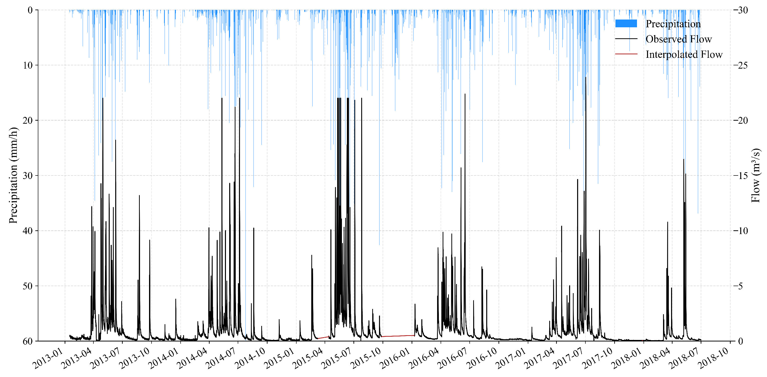
This study employs high-resolution hourly time series of spring discharge and precipitation collected from 16 January 2013 to 1 July 2018, encompassing a range of hydrological conditions and capturing both rapid and delayed flow responses characteristic of karst systems. Hourly spring discharge was measured at the G047 monitoring station, which integrates flow contributions from the upstream conduit–fissure network. Water-level data were recorded using a Levelogger Edge pressure transducer, with a stage–discharge conversion accuracy of ±2%. Data gaps, accounting for 6.9% of the total records and primarily resulting from sensor malfunctions, were addressed through linear interpolation to maintain temporal continuity in the discharge series. A binary flag variable (Flow_missing) was introduced to distinguish interpolated (value = 1) from observed (value = 0) records, allowing the modeling framework to account for uncertainty associated with missing values. Hourly precipitation data were obtained from the G037 meteorological station, which is equipped with an LS-3 vibrating-wire rain gauge offering a resolution of ±0.2 mm. Rainfall intensities exceeding 50 mm h 1 frequently generate sharp increases in spring discharge, reflecting rapid conduit-dominated quickflow. In contrast, gradual declines during dry periods reveal the contribution of slower flow components stored within the fracture–matrix continuum (Figure 2).

3. Methodology

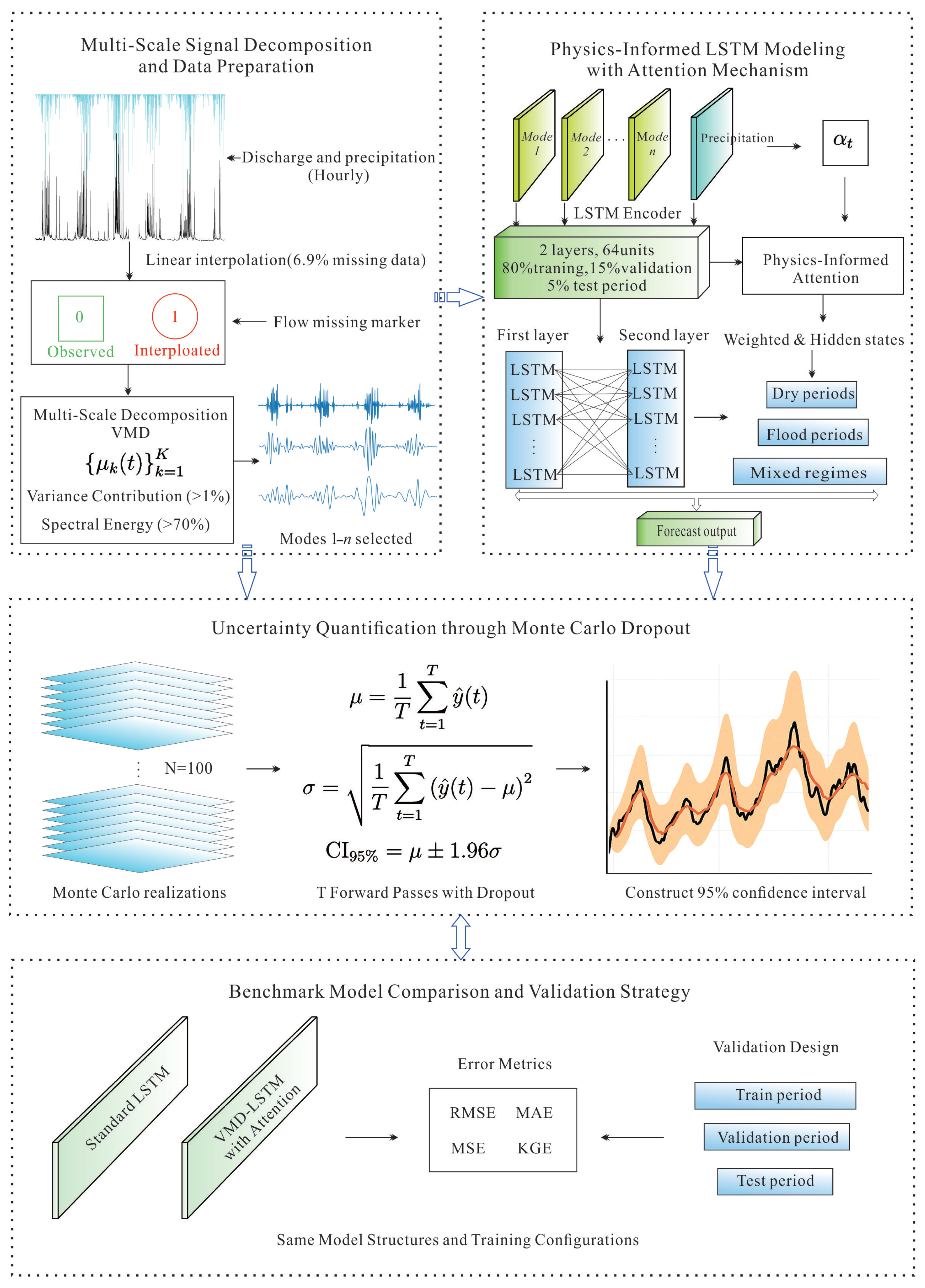
To address the inherent complexity, multi-scale variability, and nonstationarity of karst spring hydrodynamics, a physics-informed VMD-LSTM modeling framework was developed. The methodological workflow (Figure 3) comprises four integrated components: (i) Multi-scale signal decomposition and data preparation. Hourly discharge and precipitation data underwent processing, including linear interpolation for missing data (6.9%). The processed data were then decomposed into physically meaningful temporal modes using VMD. (ii) Physics-informed LSTM modeling with attention mechanism. Selected VMD modes, together with precipitation data, served as inputs to a two-layer LSTM network architecture (each layer comprising 64 units), enhanced by a physics-informed attention mechanism. This attention component dynamically assigns importance weights to temporal and hydrological features, explicitly integrating hydrological insights and allowing the model to distinguish between different flow regimes, such as dry periods, flood periods, and mixed flow regimes. The dataset was partitioned into training (80%), validation (15%), and test sets (5%) to systematically assess model robustness and generalization. (iii) Uncertainty quantification via Monte Carlo dropout. To reliably quantify predictive uncertainty, Monte Carlo dropout was implemented during inference, generating 100 stochastic forward passes through the trained LSTM model. Statistical measures of uncertainty, including prediction mean and variance, were calculated, and a 95% confidence interval was constructed, providing comprehensive insights into prediction reliability. (iv) Benchmark model comparison and validation strategy. Model performance was rigorously assessed using multiple metrics, including Root Mean Square Error (RMSE), Mean Absolute Error (MAE), Nash–Sutcliffe Efficiency (NSE), and Kling–Gupta Efficiency (KGE). The model was developed in Python 3.10 using PyTorch 2.1.0 for neural network construction and training. Data preprocessing was conducted with NumPy 2.2.4, Pandas 2.2.3, and Scikit-learn’s StandardScaler. PyTorch’s DataLoader and TensorDataset handled data batching, while Matplotlib 3.10.1 was used for visualization. Model persistence was managed with joblib 1.4.2.

3.1. Multi-Scale Signal Decomposition and Data Preparation

Due to sensor malfunctions, approximately 6.9% of the hourly spring discharge data were missing. To maintain continuity of the hydrological signals, missing values were first interpolated using piecewise linear interpolation. Subsequently, a binary quality mask m t was generated, marking observed ( m t = 0 ) and interpolated ( m t = 1 ) data points. This quality mask was incorporated as auxiliary information integrated into the attention module of the LSTM network, enabling dynamic adjustment of internal weights based on data reliability.
To capture the intrinsic multi-scale variability of the karst spring discharge, the complete time series was decomposed using VMD. This approach separates the original signal x t into a finite set of band-limited intrinsic modes { μ k ( t ) } k = 1 K by solving a variational optimization problem that minimizes each mode’s bandwidth in the spectral domain, subject to reconstructing the original signal without adding artificial noise. Each extracted mode μ k ( t ) captures hydrological variability at specific frequency scales, effectively isolating seasonal trends, quickflow responses, and high-frequency fluctuations for targeted analysis.
Modes were evaluated using three criteria to ensure their hydrological relevance: (1) a variance contribution exceeding 1%, indicating meaningful signal energy; (2) a spectral energy concentration greater than 70%, ensuring spectral coherence rather than random noise characteristics, assessed via power spectral density; and (3) a significant precipitation correlation, identified by absolute Pearson correlation coefficients | r | > 0.3 with p < 0.05 , indicating physically plausible rainfall–runoff responses. These screening criteria retained only the most physically interpretable modes as inputs for subsequent LSTM-based predictive modeling. The model is designed for multi-step-ahead forecasting of karst spring discharge at an hourly resolution, predicting discharge for the next 6 h (t + 1 to t + 6) using historical data up to the current time t. Specifically, the model takes as input the past 72 h of VMD-decomposed flow components (Mode2–Mode6), hourly precipitation, and optionally previous spring discharge observations. The typical training dataset covers approximately 5–6 years of hourly data. For operational forecasting, short sequences (e.g., the most recent 72 h inputs) are sufficient to produce near-term discharge forecasts. No future precipitation forecast is required, making the system suitable for real-time application.

3.2. Physics-Informed LSTM Modeling with Attention Mechanism

The proposed model comprises two stacked LSTM layers, each containing 64 hidden units designed to capture temporal dependencies across multiple scales. Dropout regularization (rate = 0.2) was applied between layers to prevent overfitting and enhance generalization. An attention mechanism was incorporated following the LSTM layers to selectively prioritize relevant historical information. Attention weights α t were computed via a learnable linear transformation applied to hidden states h t :
α t = exp ( w T h t ) k = 1 T exp ( w T h k )
where w R d is a learnable weight vector and T is the input sequence length. The final context vector c is constructed as a weighted sum of the hidden states as follows:
c = t = 1 T α t h t
To encourage sparsity and interpretability in the attention distribution, an entropy regularization term was added to the MSE loss function:
L total = L MSE + λ · t = 1 T α t log α t
where λ is the entropy regularization coefficient optimized via parameter tuning (see Section 4.2). The resulting context vector is passed through a fully connected output layer to produce multi-step forecasts. Compared to conventional LSTM approaches, this design improves interpretability and robustness in capturing dominant hydrological signals. To ensure data integrity, we introduced a binary weight mask based on the flow_missing flag. For interpolated discharge data points (flow_missing = 1), the corresponding loss function weight was set to zero, effectively excluding these samples from gradient computation during training.

3.3. Uncertainty Quantification Through Monte Carlo Dropout

Predictive uncertainty of the physics-informed attention-enhanced LSTM model was quantified using Monte Carlo dropout, a Bayesian approximation technique. During inference, dropout (rate = 20%) remained active, introducing stochasticity into model predictions and enabling uncertainty estimation. The number of realizations, 100, was chosen based on a sensitivity test (see Section 4.3), which demonstrated that both the RMSE and the average CI width converged and stabilized. Predictive mean ( μ ) and standard deviation ( σ ) for each time step were calculated as follows:
μ = 1 T t = 1 T y ^ t
σ = 1 T t = 1 T y ^ t μ 2
where y ^ t represents the prediction from the tth Monte Carlo realization, and T = 100 . Based on these statistics, the 95% predictive confidence interval (CI) was calculated as
CI 95 % = μ ± 1.96 σ
This uncertainty quantification approach enhances the reliability of model predictions, providing robust insights for practical hydrological decision-making. The uncertainty quantified in this study represents epistemic uncertainty arising from model variability. It is estimated using Monte Carlo dropout, which samples different neural parameter realizations during inference.

4. Results and Discussion

4.1. Multi-Scale Dynamics and Physical Interpretation of IMFs

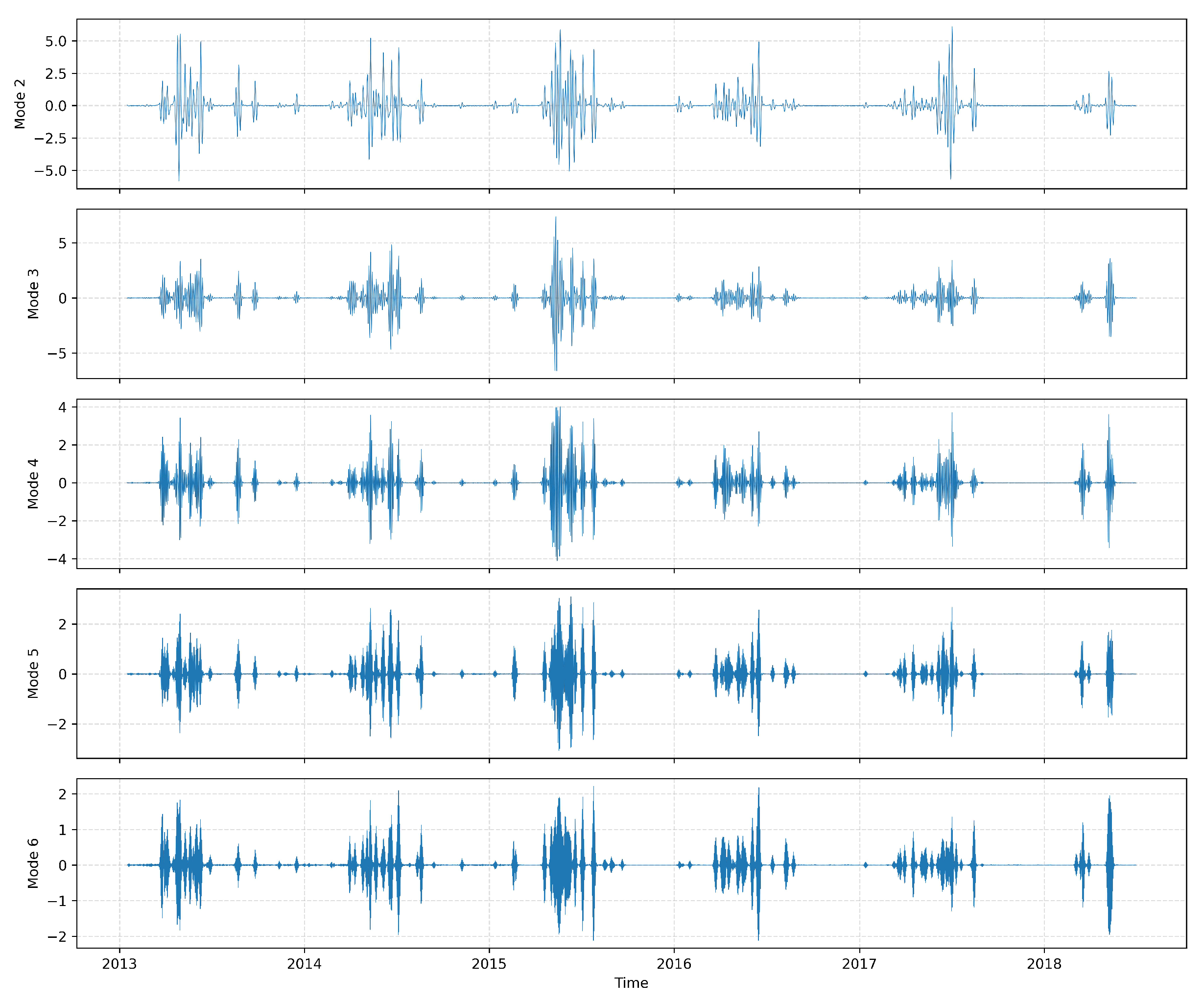
The observed karst spring discharge time series was decomposed using VMD to characterize its intrinsic multi-scale temporal variability. A total of twelve IMFs were extracted, each corresponding to a distinct frequency band. Among these, five modes (Mode2 to Mode6) were selected as inputs for the subsequent prediction modeling based on a comprehensive evaluation of their dominant periodicities, variance contributions, and hydrological interpretability (Table 1 and Figure 4). These modes were used simultaneously as multivariate inputs representing distinct hydrological processes. Collectively, these five modes accounted for approximately 32.6% of the total variance, effectively capturing the most hydrologically relevant short- to intermediate-term dynamics essential for accurate spring discharge forecasting. Modes 2 to 4 exhibited dominant periods ranging from approximately 55 to 160 h, contributing 28.4% of the total variance. These modes are interpreted as representing delayed quickflow responses governed by the epikarst and upper conduit systems, where precipitation-induced recharge is transmitted through preferential pathways with characteristic time lags. This interpretation aligns closely with the established conceptual models of karst hydrodynamics, wherein infiltration water is modulated and redistributed by storage–exchange processes within the heterogeneous subsurface structure. Modes 5 and 6 displayed shorter dominant periods of approximately 30 to 37 h, accounting for an additional 4.2% of the total variance. These modes likely reflect rapid discharge fluctuations driven by high-frequency rainfall events. In contrast, the higher-frequency modes (Mode7 and above) showed dominant periods shorter than 24 h, contributing minimally (<1%) to the overall variance. Despite their distinct spectral characteristics, these components were excluded from the model inputs due to limited physical interpretability and susceptibility to observational noise or interpolation artifacts. Similarly, the lowest-frequency mode (Mode1), with a dominant period exceeding 390 days and contributing more than 45% of the total variance, was excluded from the model training dataset. Mode1 primarily captures interannual climatic variability and large-scale seasonal storage trends, offering limited value for short- to medium-term operational forecasting. However, it was retained for qualitative assessments of long-term aquifer behavior and identification of hydroclimatic regime shifts. This targeted mode selection strategy adopted here effectively isolates physically meaningful and hydrologically significant components of the spring discharge signal, enhancing both the interpretability and predictive performance of the model. Overall, VMD provides a robust and scale-consistent approach for decomposing karst spring discharge signals, offering an ideal foundation for physics-informed hybrid modeling frameworks.

4.2. Prediction Performance of the Physics-Informed LSTM Framework

4.2.1. Model Training and Performance

The input feature set comprised five VMD components of the spring discharge (Mode2–6), along with precipitation, forming a three-dimensional input tensor X R N × T × d , where N is the number of samples, T represents the input sequence length (72 h), and d = 6 denotes the number of predictors. The prediction target was a six-hour-ahead discharge sequence, represented as Y R N × H . All the input variables were standardized using Z-score normalization. The complete hourly time series was divided into three subsets: a training set comprising 80% of the data (38,256 hourly samples, from 19 January 2013 00:00 to 28 May 2017 23:00), a validation set comprising 15% (7176 samples, from 29 May 2017 00:00 to 23 March 2018 06:00), and a test set comprising the remaining 5% (2400 samples, from 23 March 2018 07:00 to 30 June 2018 18:00). While the test set accounts for 5% of the dataset, it includes both flood and dry periods. The statistical properties of mean and standard deviation confirm their mutual representativeness. This temporal split ensured comprehensive coverage of diverse hydrological conditions for training, calibration, and evaluation. Mini-batch training was conducted with a fixed batch size of 64. The model architecture consisted of a two-layer LSTM encoder, each with 64 hidden units. A temporal attention mechanism was applied to dynamically reweight the LSTM outputs across time steps. To optimize attention sparsity, a systematic grid search was conducted over a range of entropy regularization coefficients λ   [ 0 ,   0.007 ] . This term was added to the loss function to penalize over-dispersed attention distributions and encourage focused temporal weighting. For each λ , an independent model was trained using the same data split and evaluated on the test set using RMSE, MAE, and peak RMSE.
As shown in Figure 5, while both RMSE and MAE declined with increasing λ , peak RMSE—an indicator of performance under extreme flow conditions—reached its minimum at λ = 0.005 . This suggests that moderate entropy regularization enhances the model’s ability to detect salient patterns during high-intensity events. Consequently, λ = 0.005 was selected as the final model configuration (Figure 5).
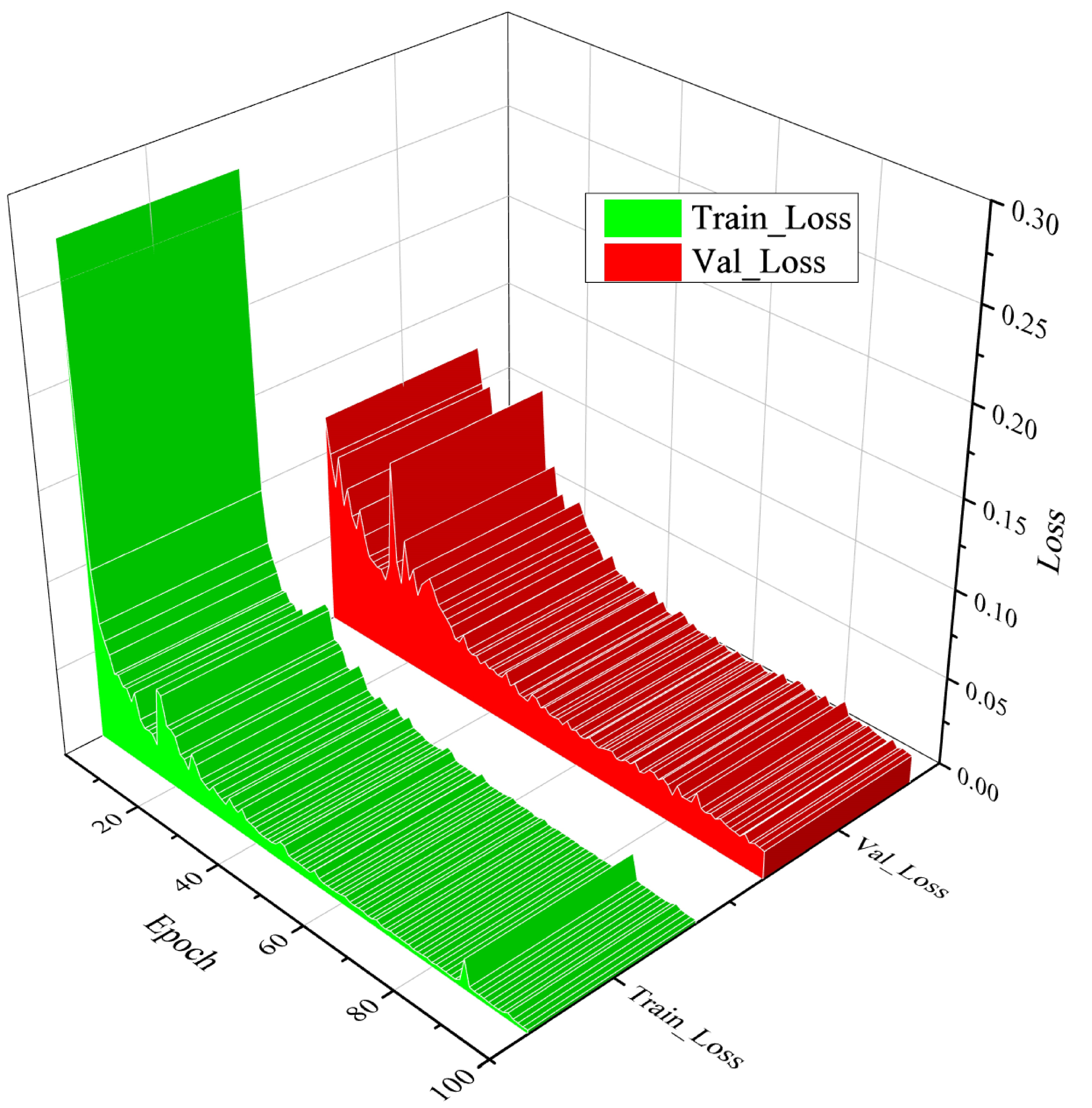
Model training was carried out over 100 epochs using the Adam optimizer. The total function comprised the MSE plus the entropy-based regularization term. Rapid convergence was observed, with validation loss decreasing from 0.1202 to 0.0496 within the first 12 epochs. Continued improvement led to a minimum validation loss of 0.0157 at epoch 97. The consistent alignment between the training and validation loss curves throughout the process indicates stable learning and minimal overfitting (Figure 6).

4.2.2. Overall Prediction Performance of the VMD-LSTM Framework

The proposed VMD-LSTM with the attention model exhibited excellent performance in reproducing both flood peaks and recession limbs, demonstrating strong predictive capability under a wide range of hydrological conditions (Figure 7). Throughout the study period, the model maintained high predictive accuracy. The RMSE was 0.083, reflecting low average deviations from the observations. The NSE reached 0.999. indicating that nearly all the variability in the observed spring discharge was captured. In addition, the KGE was 0.995, confirming the model’s accuracy in replicating the correlation, bias, and variability characteristics of the observed series.
During the training phase (Figure 8a), the model achieved near-perfect performance, with an RMSE of 0.074 and NSE of 0.999. The fitted regression line ( y = 1.00 x + 0.01 ) closely aligned with the 1:1 reference, indicating negligible bias and no overfitting. In the validation phase (Figure 8b), the performance slightly declined (RMSE = 0.250; NSE = 0.985), with the regression line ( y = 0.94 x + 0.02 ) deviating slightly below the 1:1 line. This mild underestimation of high flows likely reflects transitional hydrological states not fully represented in the training data. Nonetheless, the model maintained robust generalization performance. During the prediction phase (Figure 8c), which evaluates the model on completely unseen data, predictive skill remained high (RMSE = 0.220; NSE = 0.988). The regression line ( y = 0.98 x + 0.00 ) remained close to the ideal, highlighting the model’s ability to generalize well to future hydrological conditions.

4.2.3. Model Performance Across Hydrological Regimes

To evaluate the model robustness under different hydrological conditions, six representative periods were selected from the training, validation, and test phases, covering both flood and dry regimes. The corresponding observed and predicted discharge time series are illustrated in Figure 9. Across all the examined periods, the model maintained strong accuracy, with NSE and KGE generally exceeding 0.94, demonstrating reliable generalization. During dry periods, characterized by relatively smooth low-variability discharge, the model achieved particularly high accuracy. For instance, the Dry Validation period yielded RMSE = 0.045, MAE = 0.028, and NSE = 0.986, highlighting its effectiveness in capturing low-flow dynamics. In contrast, in the Flood Validation period, RMSE increased to 0.994 and MAE to 0.608, although NSE (0.971) and KGE (0.875) remained strong. Similarly, the Flood Prediction period exhibited moderate deviations (RMSE = 0.555; MAE = 0.252), yet retained high NSE (0.984) and KGE (0.941), indicating successful tracking of major hydrological dynamics despite slight peak-flow underestimations. These findings emphasize the value of using complementary evaluation metrics: while NSE and KGE validate the overall dynamic structural and hydrological realism, RMSE and MAE highlight potential issues in extreme event predictions.

4.3. Uncertainty Quantification

For each prediction time step, 100 stochastic realizations were generated, constructing an empirical predictive distribution. The 95% confidence intervals (CIs) were then derived as the predictive mean ± 1.96 times the standard deviation. The results demonstrate consistently high accuracy of the predicted means across the entire time series, effectively capturing both rapid rises during flood events and slow recessions during low-flow periods. The 95% CI coverage rate exceeded 96%, confirming the robustness of the uncertainty quantification under diverse hydrological conditions.
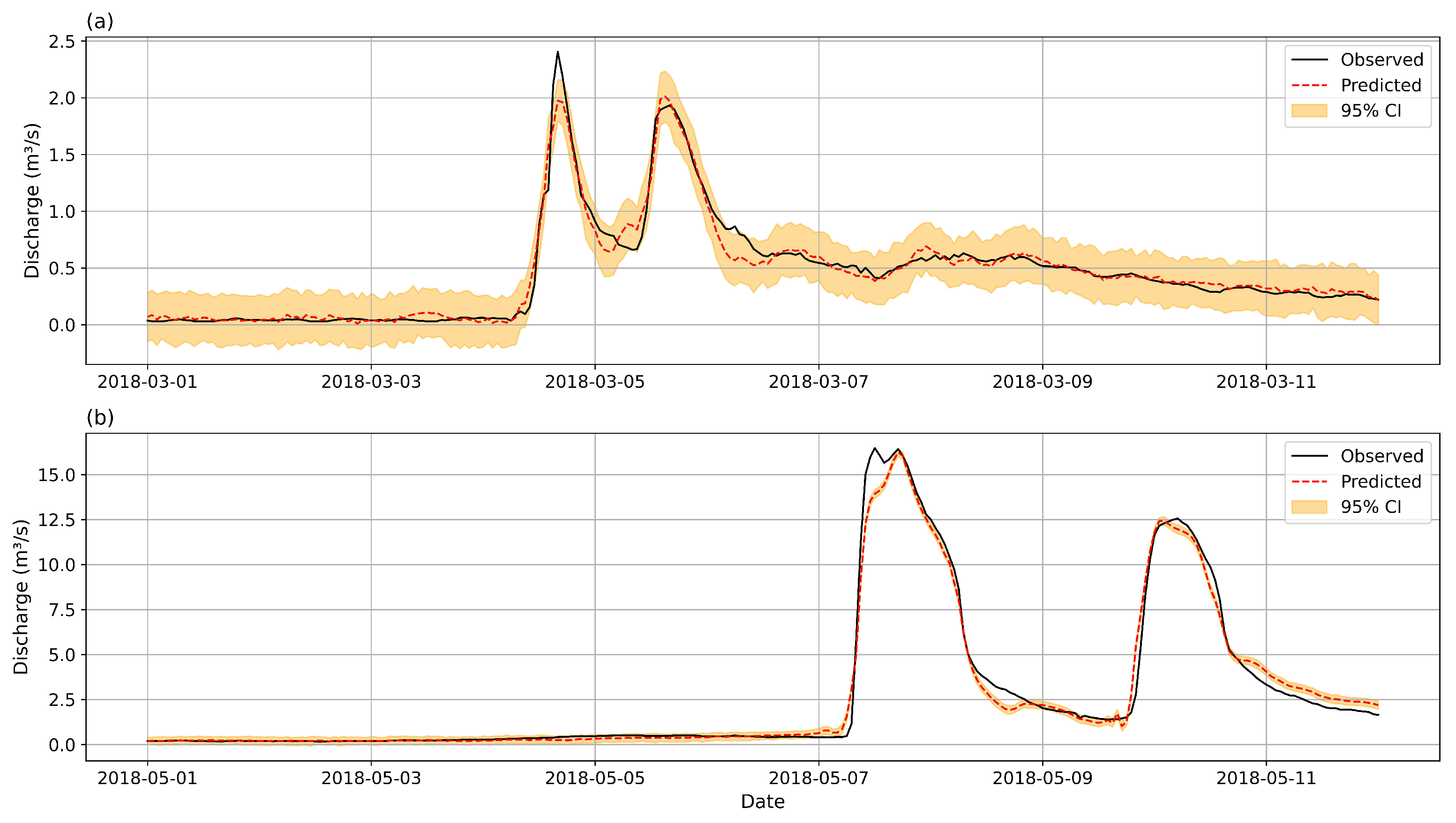
During the dry period (Figure 10a), observed discharge remains low (typically below 2.5 m3/s), with minimal fluctuations. The model closely tracked subtle variations and slow recession behavior. The associated 95% prediction intervals were relatively wide in proportion to the discharge magnitude, reflecting greater relative uncertainty under low-flow conditions. Nonetheless, the observed values consistently fell within the predicted bounds, confirming the model’s reliability in characterizing uncertainty during dry phases. In contrast, during the flood period (Figure 10b), discharge exhibited sharp rises and recession, with the peak exceeding 15 m3/s. The model demonstrates strong predictive performance, capturing both the timing and magnitude of flow peaks with high accuracy. Notably, the 95% CIs during this period were narrower relative to the discharge magnitude, indicating higher confidence and lower relative uncertainty in predicting rapidly changing flow conditions.
To evaluate the robustness of the MC dropout approach, we analyzed the sensitivity of the uncertainty estimates to the number of realizations. As shown in Figure 11, both the RMSE and the average width of the 95% confidence interval converged as the number of samples increased. The estimates stabilized after 100 realizations, confirming the reliability of the selected sampling size used in our predictions. The prediction results presented here (RMSE, NSE, 95% CI coverage, etc.) were derived under real-time forecasting conditions. The model’s inputs are limited to past data, and the outputs correspond to discharge at future time steps (t + 1 to t + 6). Therefore, these results genuinely reflect the model’s forecasting accuracy.

4.4. Comparative Analysis with Benchmark Models

To comprehensively evaluate the predictive capability of the proposed framework, we compared its performance against a baseline LSTM (denoted as “i”) and the VMD-LSTM with attention (denoted as “ii”) across the training, validation, and test phases (Table 2). The results demonstrate that the proposed model consistently outperforms the baseline across all the metrics and data subsets. During the training phase, the proposed model achieved an RMSE of 0.074 and an NSE of 0.999, reflecting near-perfect reconstruction of the training data without overfitting. In the validation phase, RMSE dropped from 0.491 (baseline) to 0.250, while NSE improved from 0.944 to 0.985, demonstrating superior generalization capability. In the test phase, which reflects the true unseen data performance, the proposed model exhibited substantial performance gains. Specifically, RMSE and MAE were reduced by 69.7% and 52.9%, respectively, compared to the baseline. NSE improved from 0.867 to 0.988 and KGE increased from 0.913 to 0.951. indicating better alignment in terms of correlation, variability, and bias. A particularly notable improvement was observed in peak RMSE (top 5% highest observed flows)—a critical metric for hydrological applications focused on flood prediction and risk management. In the test phase, peak RMSE decreased dramatically from 2.803 (baseline) to 0.923, representing a 67.1% reduction. This significant enhancement demonstrates that the integration of VMD and the attention mechanism not only enhances the overall accuracy but also substantially strengthens the model’s ability to capture extreme discharge events—typically the most challenging yet crucial aspect of hydrologic forecasting.
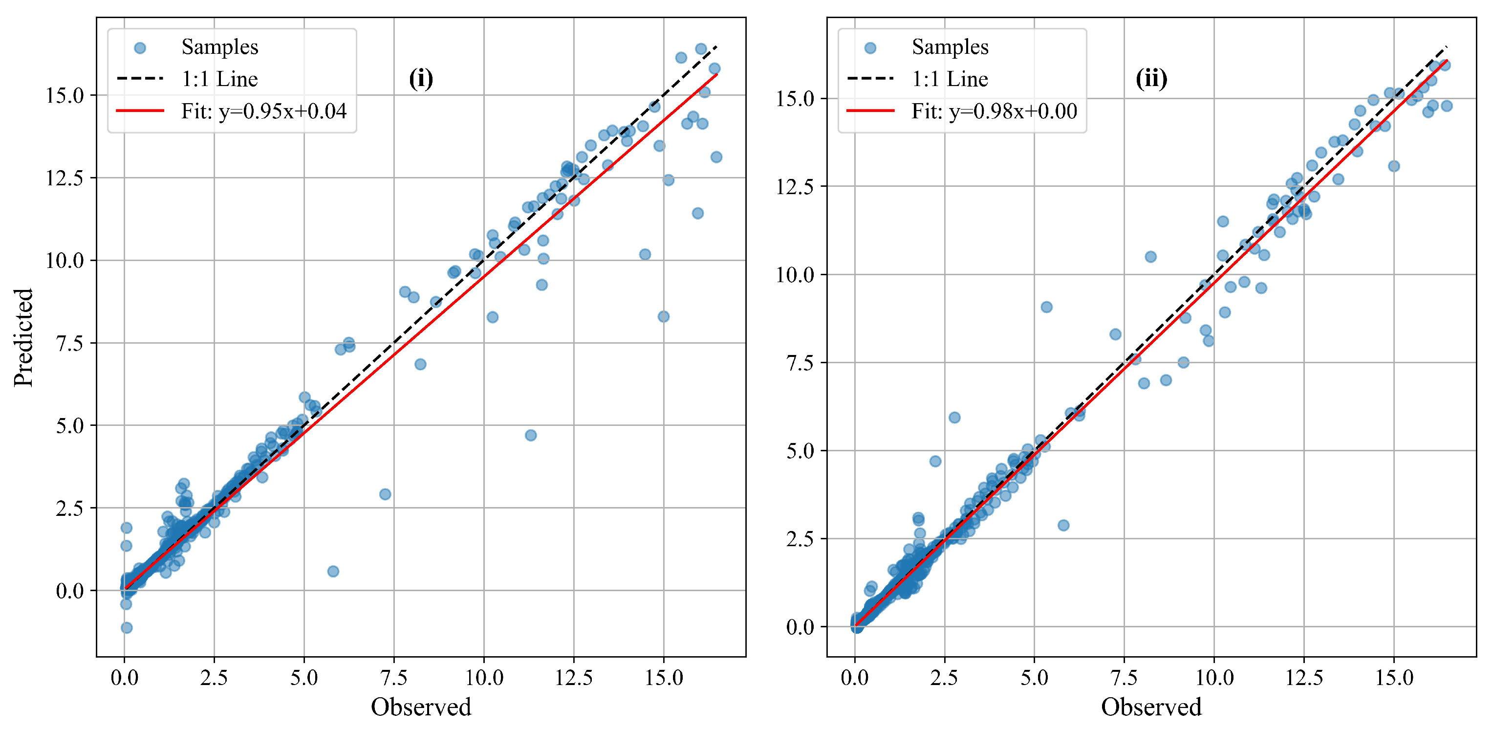
Figure 12 presents scatter plots of the predicted versus observed discharge during the test period for both models. Each subplot includes a 1:1 reference line (dashed) and a least-squares regression line (red). The proposed model displays a more concentrated distribution along the 1:1 line, indicating reduced bias and enhanced predictive accuracy. These results highlight the efficacy of combining variational mode decomposition with attention mechanisms, which improves both generalization and the model’s ability to capture baseflow and peak-flow dynamics under complex karst hydrological conditions.

5. Conclusions

This study presents a physics-informed deep learning framework that integrates VMD, an attention-augmented LSTM network, and Monte Carlo dropout to enhance the short-term forecasting of karst spring discharge. Application to the Zhaidi karst system in southern China yielded the following conclusions: (1) It improved prediction through physics-informed multi-scale modeling. The proposed VMD-LSTM with adaptive attention substantially improved the baseline LSTM, achieving higher accuracy (NSE = 0.999; RMSE = 0.083) and reducing peak prediction errors by 67%. By incorporating VMD-derived hydrologically relevant modes, the model effectively captured key short- and intermediate-scale discharge dynamics. (2) It affected the role of precipitation and attention-based physical guidance. Incorporating precipitation as an external driver substantially improved model performance during storm events. The use of a physics-informed attention mechanism enabled the model to focus on more reliable and hydrologically meaningful inputs, improving robustness under nonstationary flow conditions. (3) It included reliable uncertainty quantification under diverse regimes. Monte Carlo dropout effectively quantified the prediction uncertainty, achieving 96% coverage of the 95% Cl. This capability ensures robust and interpretable forecasting even in the presence of data gaps or noisy observations, offering practical value for real-time decision-making in karst water resource management.

Author Contributions

L.Z.: conceptualization and original draft; S.F.: conceptualization and supervision; S.L.: investigation and methodology; Z.W.: review and editing; C.L.: validation and review; Y.F.: review and editing; Y.Y.: writing and software. All authors have read and agreed to the published version of the manuscript.

Funding

This research was supported by the National Key Research and Development Program of China (2023YFB3907703_05), Karst Water Resources and Environment Academician Workstation of Guizhou Province (Qiankehepingtai-KXJZ[2024]005), and the Basic Research Fund (2022012).

Data Availability Statement

The data presented in this study are not publicly available due to institutional restrictions and data privacy considerations. However, the data may be made available from the author upon reasonable request.Requests to access the datasets should be directed to Liangjie Zhao at zhaoliangjie0@gmail.com.

Acknowledgments

We appreciate the constructive comments from the anonymous reviewers who helped to improve this manuscript.

Conflicts of Interest

The authors declare that they have no known competing financial interests or personal relationships that could have appeared to influence the work reported in this paper.

References

  1. Wali, S.U.; Usman, A.A.; Usman, A.B. Resolving challenges of groundwater flow modelling for improved water resources management: A narrative review. Int. J. Hydrol. 2024, 8, 175–193. [Google Scholar] [CrossRef]
  2. Hartmann, A.; Goldscheider, N.; Wagener, T.; Lange, J.; Weiler, M. Karst water resources in a changing world: Review of hydrological modeling approaches. Rev. Geophys. 2014, 52, 218–242. [Google Scholar] [CrossRef]
  3. Goldscheider, N.; Drew, D. (Eds.) Methods in Karst Hydrogeology: IAH International Contributions to Hydrogeology; CRC Press: Boca Raton, FL, USA, 2007; Volume 26, 190p. [Google Scholar]
  4. Jourde, H.; Wang, X. Advances, challenges and perspective in modelling the functioning of karst systems: A review. Environ. Earth Sci. 2023, 82, 396. [Google Scholar] [CrossRef]
  5. Chen, Z.; Lucianetti, G.; Hartmann, A. Understanding groundwater storage and drainage dynamics of a high mountain catchment with complex geology using a semi-distributed process-based modelling approach. J. Hydrol. 2023, 625, 130067. [Google Scholar] [CrossRef]
  6. Willard, J.; Jia, X.; Xu, S.; Steinbach, M.; Kumar, V. Integrating scientific knowledge with machine learning for engineering and environmental systems. ACM Comput. Surv. 2022, 55, 1–37. [Google Scholar] [CrossRef]
  7. Zhu, L.T.; Chen, X.Z.; Ouyang, B.; Yan, W.C.; Lei, H.; Chen, Z.; Luo, Z.H. Review of machine learning for hydrodynamics, transport, and reactions in multiphase flows and reactors. Ind. Eng. Chem. Res. 2022, 61, 9901–9949. [Google Scholar] [CrossRef]
  8. Donnelly, J.; Daneshkhah, A.; Abolfathi, S. Physics-informed neural networks as surrogate models of hydrodynamic simulators. Sci. Total Environ. 2024, 912, 168814. [Google Scholar] [CrossRef] [PubMed]
  9. Fang, L.; Shao, D. Application of long short-term memory (LSTM) on the prediction of rainfall-runoff in karst area. Front. Phys. 2022, 9, 790687. [Google Scholar] [CrossRef]
  10. Vu, M.T.; Jardani, A.; Massei, N.; Fournier, M. Reconstruction of missing groundwater level data by using Long Short-Term Memory (LSTM) deep neural network. J. Hydrol. 2021, 597, 125776. [Google Scholar] [CrossRef]
  11. Kratzert, F.; Klotz, D.; Herrnegger, M.; Sampson, A.K.; Hochreiter, S.; Nearing, G.S. Toward improved predictions in ungauged basins: Exploiting the power of machine learning. Water Resour. Res. 2019, 55, 11344–11354. [Google Scholar] [CrossRef]
  12. Gholizadeh, H.; Zhang, Y.; Frame, J.; Gu, X.; Green, C.T. Long short-term memory models to quantify long-term evolution of streamflow discharge and groundwater depth in Alabama. Sci. Total Environ. 2023, 901, 165884. [Google Scholar] [CrossRef]
  13. Lange, H.; Sippel, S. Machine Learning Applications in Hydrology. In Forest-Water Interactions; Levia, D.F., Carlyle-Moses, D.E., Iida, S., Michalzik, B., Nanko, K., Tischer, A., Eds.; Springer: Cham, Switzerland, 2020; Volume 240, pp. 233–257. [Google Scholar]
  14. Le, M.H.; Kim, H.; Adam, S.; Beling, P.; Lakshmi, V. Streamflow Estimation in Ungauged Regions Using Machine Learning: Quantifying Uncertainties in Geographic Extrapolation. Hydrol. Earth Syst. Sci. Discuss. 2022, 2022, 1–24. [Google Scholar]
  15. De Filippi, F.M.; Sappa, G. The simulation of Bracciano Lake (Central Italy) levels based on hydrogeological water budget: A tool for lake water management when climate change and anthropogenic impacts occur. Environ. Process. 2024, 11, 8. [Google Scholar] [CrossRef]
  16. Zounemat-Kermani, M.; Matta, E.; Cominola, A.; Xia, X.; Zhang, Q.; Liang, Q.; Hinkelmann, R. Neurocomputing in surface water hydrology and hydraulics: A review of two decades retrospective, current status and future prospects. J. Hydrol. 2020, 588, 125085. [Google Scholar] [CrossRef]
  17. Wu, M.; Liu, P.; Liu, L.; Zou, K.; Luo, X.; Wang, J.; Xia, Q.; Wang, H. Improving a hydrological model by coupling it with an LSTM water use forecasting model. J. Hydrol. 2024, 636, 131215. [Google Scholar] [CrossRef]
  18. Lawal, Z.K.; Yassin, H.; Teck, D.; Lai, C.; Idris, A.C. Coastal Wave Modeling and Forecasting with LSTM Optimization for Sustainable Energy Harvesting. 2023. Available online: https://www.preprints.org/manuscript/202304.0282/v2 (accessed on 18 May 2023).
  19. Tobin, B.W.; Polk, J.S.; Arpin, S.M.; Shelley, A.; Taylor, C. A conceptual model of epikarst processes across sites, seasons, and storm events. J. Hydrol. 2021, 596, 125692. [Google Scholar] [CrossRef]
  20. Liu, J.; Xu, T.; Lu, C.; Yang, J.; Xie, Y. Variational mode decomposition coupled LSTM with encoder-decoder framework: An efficient method for daily streamflow forecasting. Earth Sci. Inform. 2025, 18, 38. [Google Scholar] [CrossRef]
  21. Wang, J.; Wang, X.; Lei, X.H.; Wang, H.; Zhang, X.H.; You, J.Y.; Tan, Q.F.; Liu, X.L. Teleconnection analysis of monthly streamflow using ensemble empirical mode decomposition. J. Hydrol. 2020, 582, 124411. [Google Scholar] [CrossRef]
  22. Renard, B.; Kavetski, D.; Leblois, E.; Thyer, M.; Kuczera, G.; Franks, S.W. Toward a reliable decomposition of predictive uncertainty in hydrological modeling: Characterizing rainfall errors using conditional simulation. Water Resour. Res. 2011, 47, W11516. [Google Scholar] [CrossRef]
  23. Zhou, R.; Wang, Q.; Jin, A.; Shi, W.; Liu, S. Interpretable multi-step hybrid deep learning model for karst spring discharge prediction: Integrating temporal fusion transformers with ensemble empirical mode decomposition. J. Hydrol. 2024, 645, 132235. [Google Scholar] [CrossRef]
  24. Zhang, W.; Duan, L.; Liu, T.; Shi, Z.; Shi, X.; Chang, Y.; Wang, G. A hybrid framework based on LSTM for predicting karst spring discharge using historical data. J. Hydrol. 2024, 633, 130946. [Google Scholar] [CrossRef]
  25. An, L.; Hao, Y.; Yeh, T.-C.J.; Liu, W.; Zhang, B. Simulation of karst spring discharge using a combination of singular spectrum analysis and ensemble empirical mode decomposition with LSTM modeling. Environ. Earth Sci. 2020, 79, 353. [Google Scholar]
  26. Wang, J.; Zhang, B.; Hao, Y.; Zhang, B.; Zhang, C.; Guo, C.; Zhu, Y. Spring flow prediction model based on VMD and attention mechanism LSTM. In International Conference in Communications, Signal Processing, and Systems; Springer: Singapore, 2023; pp. 111–120. [Google Scholar]
  27. Wei, X.; Chen, M.; Zhou, Y.; Zou, J.; Ran, L.; Shi, R. Research on optimal selection of runoff prediction models based on coupled machine learning methods. Sci. Rep. 2024, 14, 32008. [Google Scholar] [CrossRef]
  28. Xu, D.M.; Liao, A.D.; Wang, W.; Tian, W.C.; Zang, H.F. Improved monthly runoff time series prediction using the CABES-LSTM mixture model based on CEEMDAN-VMD decomposition. J. Hydroinform. 2024, 26, 255–283. [Google Scholar] [CrossRef]
  29. Ding, Y.; Zhu, Y.; Feng, J.; Zhang, P.; Cheng, Z. Interpretable spatio-temporal attention LSTM model for flood forecasting. Neurocomputing 2020, 403, 348–359. [Google Scholar] [CrossRef]
  30. Li, W.; Liu, C.; Xu, Y.; Niu, C.; Li, R.; Li, M.; Tian, L. An interpretable hybrid deep learning model for flood forecasting based on Transformer and LSTM. J. Hydrol. Reg. Stud. 2024, 54, 101873. [Google Scholar] [CrossRef]
  31. Masih, I.; Maskey, S.; Uhlenbrook, S.; Smakhtin, V. Assessing the impact of areal precipitation input on streamflow simulations using the SWAT Model 1. JAWRA J. Am. Water Resour. Assoc. 2011, 47, 179–195. [Google Scholar] [CrossRef]
  32. Dai, Z.; Zhang, M.; Nedjah, N.; Xu, D.; Ye, F. A hydrological data prediction model based on LSTM with attention mechanism. Water 2023, 15, 670. [Google Scholar] [CrossRef]
  33. Zhang, C.; Zhou, Y.; Lu, F.; Liu, J.; Zhang, J.; Yin, Z.; Ji, M.; Li, B. Assessing the performance and interpretability of the CNN-LSTM-Attention model for daily streamflow forecasting in typical basins of the eastern Qinghai-Tibet Plateau. Sci. Rep. 2025, 15, 82. [Google Scholar] [CrossRef]
  34. Zhou, R.; Zhang, Y. Predicting and explaining karst spring dissolved oxygen using interpretable deep learning approach. Hydrol. Process. 2023, 37, e14948. [Google Scholar] [CrossRef]
  35. Alizadeh, F.; Roushangar, K.; Adamowski, J. Investigating monthly precipitation variability using a multiscale approach based on ensemble empirical mode decomposition. Paddy Water Environ. 2019, 17, 741–759. [Google Scholar] [CrossRef]
  36. Longyang, Q.; Choi, S.; Tennant, H.; Hill, D.; Ashmead, N.; Neilson, B.T.; Xu, T. An attention-based explainable deep learning approach to spatially distributed hydrologic modeling of a snow dominated mountainous karst watershed. Water Resour. Res. 2024, 60, e2024WR037878. [Google Scholar] [CrossRef]
  37. Liu, J.; Koch, J.; Stisen, S.; Troldborg, L.; Schneider, R.J. A national scale hybrid model for enhanced streamflow estimation—Consolidating a physically based hydrological model with long short-term memory networks. Hydrol. Earth Syst. Sci. Discuss. 2024, 28, 2871–2893. [Google Scholar] [CrossRef]
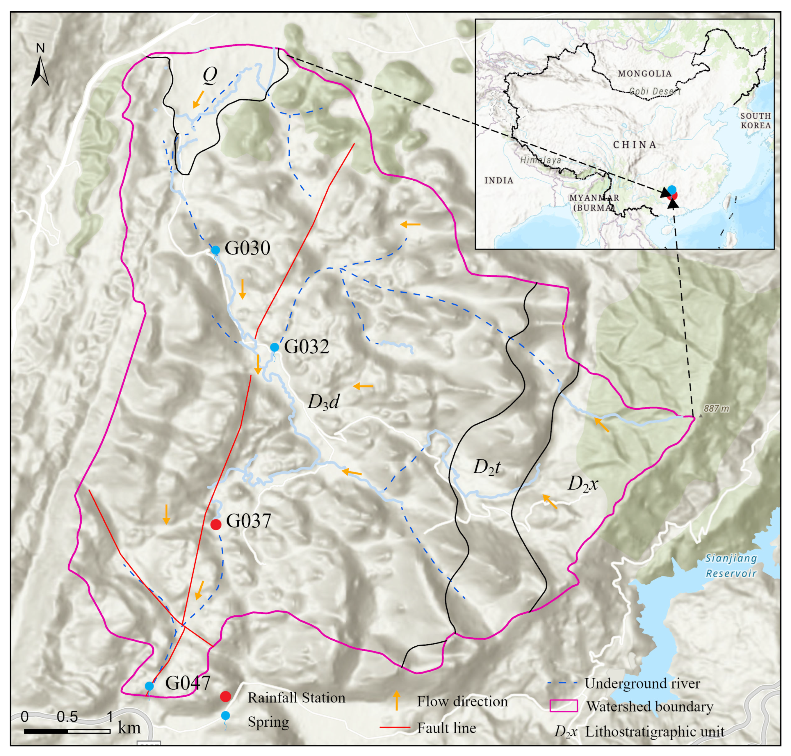
Figure 1. Geological and hydrological setting of the Zhaidi karst system.
Water 17 02043 g001
Figure 2. Hourly time series of precipitation and spring discharge from 2013 to 2018.
Water 17 02043 g002
Figure 3. Schematic overview of the proposed physics-informed VMD-LSTM with attention framework for karst spring flow forecasting.
Water 17 02043 g003
Figure 4. Multi-scale decomposition of observed karst spring discharge using VMD.
Water 17 02043 g004
Figure 5. Comparison of model performance on the test set under varying entropy regularization coefficients λ .
Water 17 02043 g005
Figure 6. Training and validation loss curves over 100 epochs.
Water 17 02043 g006
Figure 7. Observed versus predicted karst spring discharge over the full study period.
Water 17 02043 g007
Figure 8. Scatter plots comparing observed and predicted spring discharge.
Water 17 02043 g008
Figure 9. Observed and predicted discharge during six representative periods spanning flood and dry regimes across all modeling phases.
Water 17 02043 g009
Figure 10. Observed and predicted spring discharge values with 95% Cl under (a) flood and (b) dry periods.
Water 17 02043 g010
Figure 11. Sensitivity of MC dropout results to the number of realizations.
Water 17 02043 g011
Figure 12. Scatter plots comparing test-stage predictions between the baseline LSTM model (i) and the proposed framework (ii).
Water 17 02043 g012
Table 1. Characteristics and preliminary hydrological interpretations of the 12 intrinsic mode functions (IMFs) derived from VMD.
ModeVariance Contribution (%)Dominant Period (h/d)Preliminary Hydrological Interpretation
Mode145.869561.6/398.4Interannual variability and seasonal trends
Mode213.99160.4/6.7
Mode38.9390.5/3.8Medium-scale quickflow response
Mode45.4854.8/2.3
Mode52.7637/1.5Rapid to intermediate flow processes
Mode61.4030.1/1.3
Mode70.7621.6/0.9
Mode80.4316.8/0.7Variance Contribution < 1%
Mode90.2512.4/0.5
Mode100.139/0.4
Mode110.076.8/0.3
Mode120.045.5/0.2
Table 2. Performance of the baseline LSTM (i) and proposed framework (ii) across different modeling phases.
MetricTrain (i)Train (ii)Validation (i)Validation (ii)Test (i)Test (ii)
RMSE0.1420.0740.4910.2500.7260.220
MAE0.0570.0470.1460.0810.1550.073
NSE0.9960.9990.9440.9850.8670.988
KGE0.9800.9800.9260.9360.9130.951
Peak_RMSE (5%)0.4120.2181.7371.0192.8030.923
Disclaimer/Publisher’s Note: The statements, opinions and data contained in all publications are solely those of the individual author(s) and contributor(s) and not of MDPI and/or the editor(s). MDPI and/or the editor(s) disclaim responsibility for any injury to people or property resulting from any ideas, methods, instructions or products referred to in the content.