Disentangling the Source of Uncertainty in Monthly Streamflow Predictions: A Case Study of Riu Mannu di Narcao Basin, Sardinia Region, Italy

Abstract

This study quantifies the uncertainty in monthly streamflow predictions under future climate scenarios in two periods (near and far future) for the Riu Mannu di Narcao basin in Sardinia, Italy. The sources of uncertainty include the hydrological model structure, model parameters, and variability in climatic inputs derived from global and regional climate models (GCM-RCM coupling) and representative concentration pathways (RCPs). Three conceptual and lumped hydrological models (GR3M, ABCD, and IHACRES) were combined with four climate models and two RCPs (RCP 4.5 and RCP 8.5) to assess future streamflow. Monte Carlo simulations were performed to evaluate parameter uncertainty, and the analysis of variance (ANOVA) method was applied to quantify the different sources of uncertainty. The results reveal that, as a single source, GCM-RCM coupling is the largest contributor, accounting for 47.32% (54.64%) of total near (far) future monthly streamflow projection uncertainties, followed by the hydrological model structure at 16.02% (21.09%), RCP scenarios at 15.35% (8.54%), and parameter uncertainty at 0.79% (1.39%). A consistent decline in median monthly streamflow is projected, especially during winter months (December to February), raising a concern about water availability in the region. Our study quantified different sources of uncertainty in monthly streamflow predictions under climate change, disentangling the roles of the hydrological model, model parameters, climate model, and climate scenario for reliable future streamflow projections.

1. Introduction

Freshwater resources are crucial for human development, ecosystem health, and economic growth, supporting both terrestrial and aquatic ecosystems [1]. However, these resources are increasingly constrained by anthropogenic activities [2]. Climate change further intensifies water scarcity by altering hydrological process like streamflow, groundwater recharge, and evapotranspiration, particularly in regions with limited freshwater availability [3,4].

Numerous studies predict that future climate change will increase mean temperatures and decrease mean precipitation in the Mediterranean region, which has been designated as one of the world’s most prominent “hot spots” for climate change impacts [4,5,6,7,8]. It will also increase potential evapotranspiration, which is triggered by rising temperatures, and these changes may have a non-linear and combined effect on streamflow components [4,9]. Consequently, a number of researchers agree that the projected future streamflow trend is expected to decline, which would increase the risk of drought and raise management challenges related to water resources in the future, particularly if the area is highly populated [7,9,10]. According to Khadka, D. and Richardson, C.M. [11,12], future climate change would intensify the hydrological cycle and alter the distribution of freshwater resources across different temporal and spatial scales. Therefore, predicting streamflow within the context of climate change is crucial for sustainable water resource management, helping to mitigate the most severe impacts and develop effective adaption strategies.

Projecting future streamflow remains a significant challenge for water resource researchers, given the various sources of uncertainties [13]. These uncertainties generally can be attributed to as natural climate variability, representative concentration pathways (RCPs), a global climate model (GCM) structure, regional climate model (RCM), GCM-RCM coupling, hydrological model structure, parametric uncertainty, and hydrometric uncertainty resulting from observational data used to calibrate the models [14,15]. Among these, researchers often focus on quantifying four major uncertainties: (i) RCP scenarios, (ii) GCM-RCM coupling, (iii) hydrological model structural uncertainty, and (iv) parametric uncertainty. The first two sources of uncertainty are strictly related to climate change forcing, namely, climate change scenarios, GCM and RCM structures, parameterization, and the nesting scheme [14,16], while the last two sources are introduced by the choice of the hydrological modelling approach. Overall, these uncertainties create complexities for local water decision-makers when planning for the sustainable management of water resources [13,17]. It is therefore advised to properly quantify the projection uncertainties.

In hydrological models, the selection of model mechanisms, algorithms, parameters, and temporal and spatial scales of modelling can have a substantial impact on the outcomes and is a key source of uncertainty in model predictions [18,19,20]. Therefore, it is crucial to thoroughly evaluate the model output to determine the degree of predictive uncertainty present in the model [16,21,22]. Parametric uncertainty is one of the most frequent types of uncertainty in hydrological models, but it can be controlled to improve the model’s robustness and reliability [23]. According to Renard, B. and Teweldebrhan, A.T. [21,22], parametric uncertainty illustrates the difficulty in defining precise values for the model parameters. Several parameter sets could be linked to the same optimal efficiency metric. This concept, known as “equifinality”, reflects the idea that multiple plausible representations of a model are difficult to dismiss and must be considered when assessing uncertainty in predictions [24,25].

The roles of climate models’ variability, the hydrological model structure, parametric uncertainty, and RCP scenarios have been highlighted by many authors as the main sources of uncertainty in streamflow predictions under climate change [13,14,16,17,26]. For instance, in 12 major river basins around the world, Vetter, T. [27] used the analysis of variance (ANOVA) method to assess the sources of uncertainty in projected two runoff quantiles: low flows and high flows under climate change. The results shows that GCM contributed the most uncertainty (30 to 65%), followed by hydrological model uncertainty (20 to 35%). Lee, S. [16] used the ANOVA method to quantify the uncertainty in monthly streamflow predictions under climate change. They concluded that the variability of GCM projections contributed the most to the total uncertainty (48%), followed by parameter uncertainty (23%) and the RCP scenario (16%). In a recent research, Ye, Y. [28] evaluated the uncertainty in three runoff quantiles, low flow, mean flow, and high flow, under climate change and found that internal climate variability was the largest contributor to uncertainty (50%), followed by uncertainty in hydrological models (12.9%) and the RCP scenario (7.3%). Furthermore, in quantifying uncertainties in streamflow quantiles, Mehboob, M.S. [29] highlighted that GCM was the main source of uncertainty, accounting for 64% of the total uncertainty, followed by parameter uncertainty (12%).

However, few studies have simultaneously quantified the contribution to uncertainty from all sources in a comprehensive analysis, e.g., considering the relative sources from RCP scenarios, GCM-RCM coupling, hydrological models, and corresponding parameters. Within this context, the novelty of this work lies in extending the quantification of the uncertainty from different sources for monthly streamflow predictions. With this aim, the analysis of variance (ANOVA) method was used to quantify the impact of each of four key uncertainties: climate change forcing (RCP scenarios and GCM-RCM coupling), the hydrological model structure, and parameter uncertainty. The results are presented in terms of the relative contribution of each source of uncertainty to the relative variability in monthly streamflow, i.e., the proportion of each source’s serial variation to the total variance. The novelty of this work is thus further explained by the three main ideas and actions listed below.

• We selected best 100 equifinal NSE values with their associated parameter sets alongside with four GCM-RCM coupling models, three hydrological models, and two RCP scenarios for both the near and far future, and we simulated future monthly streamflow, i.e., 2400 simulations from (100 PARs × 4 GCM-RCMs × 3 HMs × 2 RCPs).
• Since there is uncertainty in the 2400 streamflows that we simulated using a combination of 100 PARs, four CMs, three HMs, and two RCPs, we quantified the contributions of each of the four major uncertainty sources and their interaction effects (IEs) to the overall uncertainty in the monthly streamflow predictions. We employed the ANOVA approach to do this.
• ANOVA breaks down the total uncertainty of the output and assigns its components to different sources of uncertainty and their interactions. Consequently, we calculated the percentage of variance that was explained by the model parameters, climate model, hydrological model, RCP scenario, and their interaction effects.

Climate change data uncertainty is examined using four climate models from the EURO-CORDEX domain, which Mascaro, G. [30] identified as providing the best hydro-climatic forcings for precipitation and temperature in the Sardinia region, while as regarding representative concentration pathway scenarios, RCP 4.5 and 8.5 were selected. Hydrological model structure uncertainty is assessed using three conceptual lumped hydrological models, namely, GR3M, IHACRES, and ABCD [31,32,33], all calibrated via Monte Carlo simulation to accurately capture the hydrological signal in the study area. To address parametric uncertainty, automatic calibration through Monte Carlo simulations is employed, generating multiple parameter sets.

The Riu Mannu di Narcao catchment, the case study, is crucial to maintaining the freshwater supply for several of the southern Sardinian economic centres, including those for domestic and agricultural use. Despite its significance, no prior research has evaluated freshwater availability in this basin under future climate change conditions. The current study aims to address that gap by assessing streamflow and the associated uncertainties under climate change scenarios. The findings will provide valuable insights for local water agencies and decision-makers, helping them implement effective water exploitation policies and mitigate drought risks.

2. Materials and Methods

2.1. Study Area and Datasets

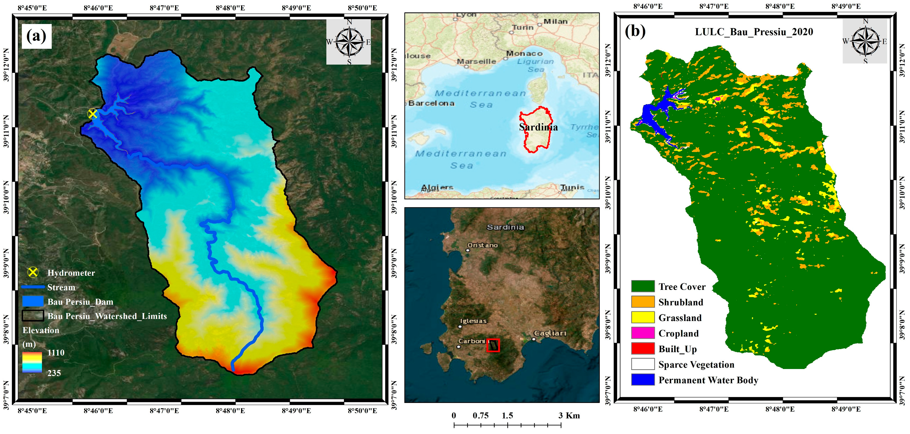
The Riu Mannu di Narcao watershed was chosen as the case study. Water resources in the study area are crucial for both environmental services and local economic activities. The Riu Mannu di Narcao watershed covers an area of 28 km², with an elevation ranging from 235 to 1110 m, as shown in Figure 1a. The Sardinia Water Authority monitored key hydrological variables, temperature, evaporation, and precipitation within the basin from 2010 and 2020, providing essential data for understanding the region’s water balance as the annual precipitation, which ranges from 436 mm to 1144 mm, with a mean value of 680 mm. Streamflow time series from 2010 and 2020 were derived by applying the water balance equation to a reservoir within the catchment to reconstruct the inflow data. We used water level time series from the Bau Pressiu Dam, a reservoir providing freshwater for both irrigation and drinking purposes. Located within the municipalities of Nuxis, Narcao, and Siliqua (province of Southern Sardinia), the dam has been operational since 2006 and has a total storage of around 10.2 million cubic meters. The water supply data were provided by the local water authority and together with the evaporation from the surface (reconstructed by the Thornthwaite method) allowed us to assess streamflow incoming from the basin. The mean monthly streamflow per unit area in the Riu Mannu di Narcao basin results in about 23 mm/month, while the annual streamflow in the basin ranges from 111 to 537 mm/year, with an average of 280 mm/year. The discharge value is smaller than the mean monthly value in over 70% of months, particularly during the summer, when the basin experiences significant hydrological stress. The land use land cover (LULC) in the Riu Mannu di Narcao basin is predominantly tree cover, accounting for over 85% of the total, followed by grass land and shrub land, as shown in Figure 1b.

2.2. Climate Models

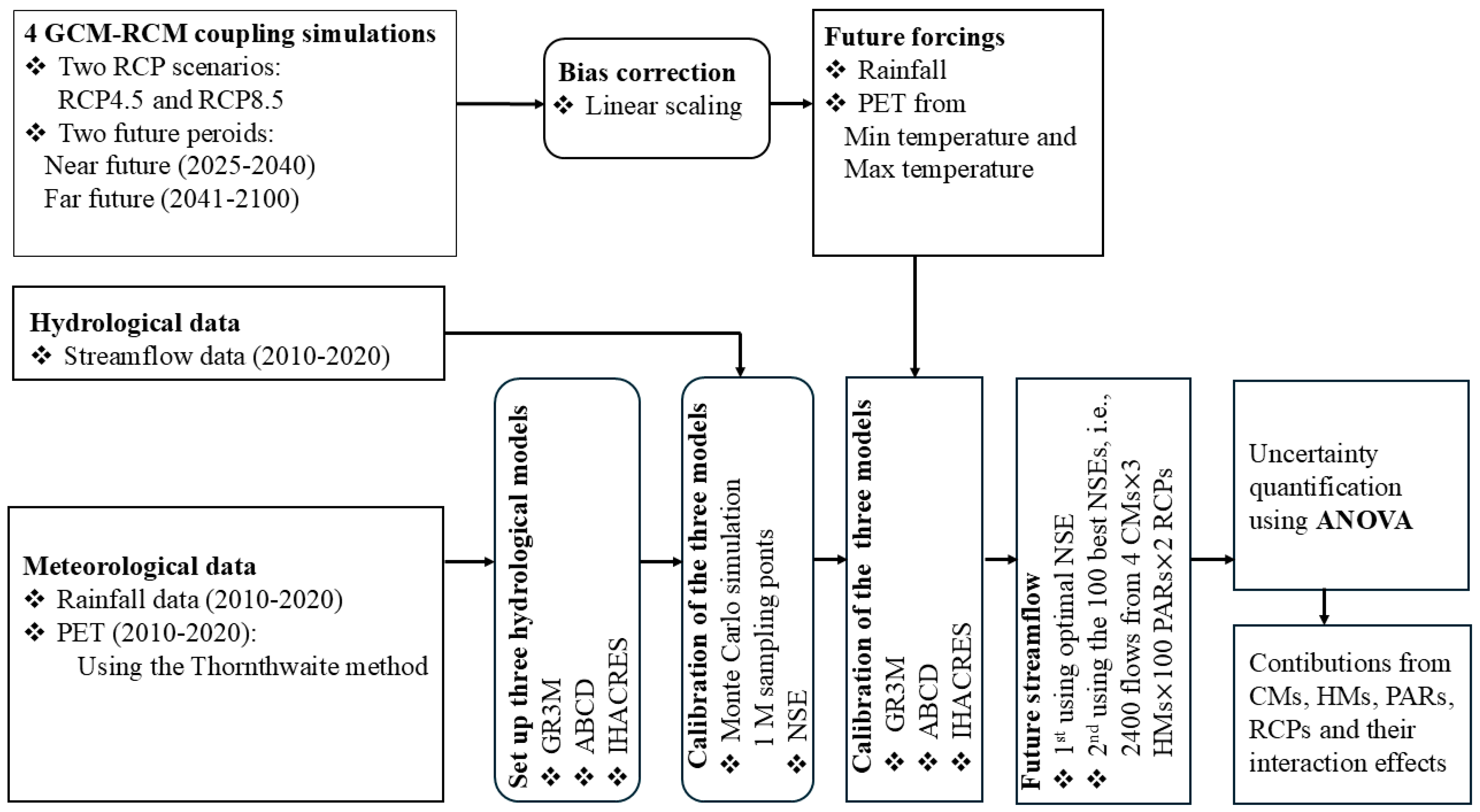
The overall framework for climate change impact evaluation process is presented in Figure 2. This study uses four climate models as inputs for future water resource predictions. These models were selected on the basis of the regional validation described by Mascaro, G. [30], since they provide a reliable representation of historical precipitation and temperature for the Sardinia basins. These four climate models were chosen because the climatology means’ spatial pattern is comparatively well-produced and associated with observations in Sardinia catchments. Specifically, the following four GCM-RCM combinations from the EURO-CORDEX domain were employed, with a horizontal grid spacing of 0.11° and a daily temporal resolution: CNRM-CM-CCLM4, EC-EARTH-RACMO22E, CNRM-CM-RCA4, and HadGEM2-ES-RACMO22E.

As known, EURO-CORDEX conducts two sets of experiments with coupled GCM-RCM: (i) the “Historical experiment”, which generates the historical climate in the period of 1950–2005, and (ii) the “Scenarios”, which projects future climate conditions (2025–2100) under different representative concentration pathways (RCPs) from CMIP5.

The historical simulation of the climate forcings, including precipitation, minimum and maximum temperatures, for the Riu Mannu di Narcao basin have been bias corrected to match with observed monthly data in the historical period of 1950–2005. The climatology site of ARPAS (regional agency for the protection of the environment of Sardinia) provided the baseline data for minimum and maximum temperatures and precipitation. The reference stations are Nuxis (for precipitation), Rosas (for minimum temperature), and Terraseu (for maximum temperature). All these stations are located very close to the Bau Pressiue Dam.

Two representative concentration pathways (RCPs) are considered in this study: RCP4.5, which assumes that greenhouse gas emissions would increase by +4.5 W/m² relative to pre-industrial values, and RCP8.5, which assumes that emissions will increase by +8.5 W/m² by the year 2100. The four climate scenarios that have been simulated are the near future (2025–2040) and the far future (2041–2100) projections for both the RCP4.5 and RCP8.5 scenarios.

The current study uses the linear scaling technique, which bases its monthly correction values on the discrepancy between observed and raw data from the climate model in the historical period to correct bias in temperature and precipitation. Specifically, we used additive correction for temperature and multiplicative correction for precipitation, according to the following equations:

$$T_{cor,m,d}=T_{raw,m,d}+\mu \left(T_{obs,m}\right)-\mu \left(T_{raw,m}\right)$$

(1)

$$P_{cor,m,d}=P_{raw,m,d}\times {\displaystyle \frac{\mu \left(P_{obs,m}\right)}{\mu \left(P_{raw,m}\right)}}$$

(2)

where $T_{cor,m,d}$ and $P_{cor,m,d}$ are the bias-corrected temperature and rainfall, respectively, on the $d^{th}$ day of $m^{th}$ month, and $T_{raw,m,d}$ and $P_{raw,m,d}$ are the raw temperature and rainfall, respectively, on the $d^{th}$ day of $m^{th}$ month. $\mu \left(.m\right)$ indicates the monthly mean value of the variable within brackets in the given month.

2.3. Hydrological Models’ Descriptions

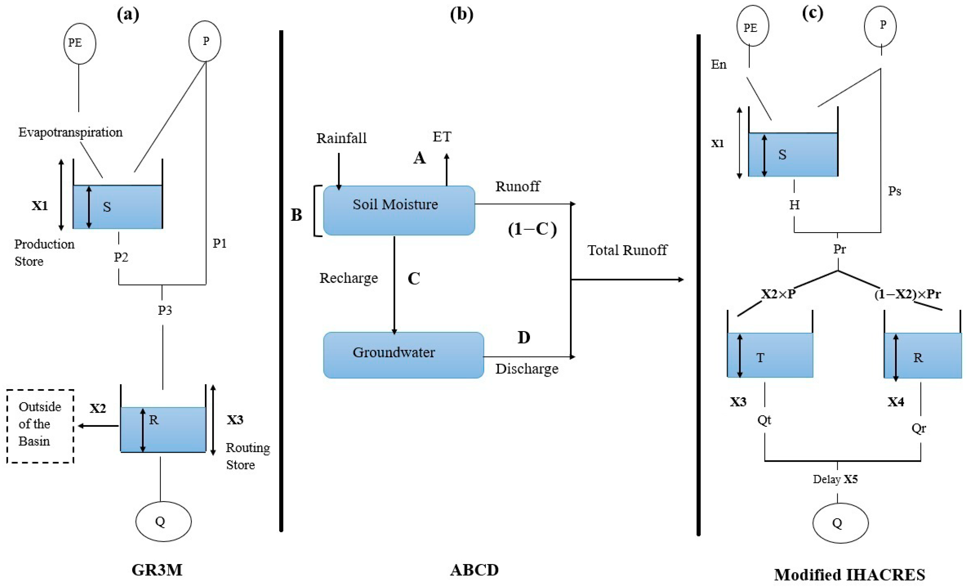
For this study, three conceptual and lumped hydrologic models with different levels of complexity were selected to predict the streamflow, namely, GR3M, ABCD, and IHACRES models. Streamflow, groundwater, and soil moisture dynamics are often predicted using these models, which have also been demonstrated to be effective tools for managing water resources, evaluating water availability, and assessing the impacts of climate change. A brief description of each model is provided in the following.

2.3.1. GR3M Model

We propose here an enhanced version of the GR2M conceptual rainfall–runoff model first introduced in the late 1980’s to better reproduce erratic hydrological regimes. Several researchers have contributed to its development, with significant updates provided by Mouelhi, S. [32]. The original GR2M model was designed with two parameters: ${\mathit{X}}_1$, which governs the maximum soil moisture capacity; and ${\mathit{X}}_2$, which controls the water exchange between the basin and neighbouring basins. While the GR2M model was effective for non-erratic hydrological regimes, it had limitations in simulating runoff processes in catchments with complex hydrological characteristics [32,34].

To address these limitations and improve the model’s ability to simulate streamflow in catchments with erratic hydrological regimes, we extended the GR2M model by introducing a third parameter (${\mathit{X}}_3$), which represents the maximum capacity of the routing reservoir. This improvement allows the proposed model, here referred to as GR3M, to better capture the dynamic routing of water within the basin, a critical component in areas where seasonal variability plays a significant role in streamflow patterns, such as the Mediterranean climate. As illustrated in Figure 3a, the additional parameter enhances the model’s flexibility and ability to represent complex flow processes by adjusting the capacity of the routing store dynamically. Thus, in summary, the key parameters in the GR3M model are ${\mathit{X}}_1$, the maximum soil moisture capacity; ${\mathit{X}}_2$, the water exchange coefficient between the basin and neighbouring basin; and ${\mathit{X}}_3$, the maximum capacity of the routing reservoir (newly introduced in GR3M).

The GR3M model operates on a monthly time step by simulating water flow between two zones: the upper zone, which represents the soil moisture content, and a lower zone, which acts as a routing reservoir. Rainfall first infiltrates the soil, raising the soil moisture content ($S$). If the soil reaches saturation, excess rainfall or surface water flow appears ($P_1$). Deep percolation or subsurface flow ($P_2$) further reduces the soil moisture ($S$), with evapotranspiration acting as the main water loss from the upper zone. When water from subsurface runoff ($P_2$) and excess rainfall ($P_1$) combine, surface runoff ($P_3$) emerges. This surface runoff ($P_3$), along with the water from the previous month ($R$), are routed into the lower zone (routing reservoir). The water flowing out of this routing reservoir is controlled by parameter ${\mathit{X}}_2$ (water exchange coefficient). The flexibility introduced by ${\mathit{X}}_3$ allows for a more dynamic representation of water retention in the routing reservoir, with the model adjusting the flow based on this parameter’s value.

If ${\mathit{X}}_2$ is 0, all water leaves the basin and reaches the neighbouring basin, while if ${\mathit{X}}_2$ is 1, water is fully retained within the basin. The enhanced routing process improves the model’s ability to simulate streamflow responses under varying conditions. The streamflow ($Q$) generated by the model is calculated using Equation (3):

$$Q={\displaystyle \frac{R_2^2}{R_2+{\mathit{X}}_3}}$$

(3)

where $R_2$ is the routed water based on the exchange coefficient.

The GR3M model thus provides greater flexibility in hydrological simulations, particularly in regions with pronounced seasonal variations. By allowing the routing reservoir capacity to vary, the GR3M model offers a more realistic representation of how water moves through the landscape, making it a valuable tool for studying catchments with complex hydrological characteristics.

2.3.2. ABCD Water Balance Model

The ABCD model is a lumped and conceptual monthly hydrological model that was developed by Jr, H.A.T. [31]. It is a nonlinear hydrological model that estimates streamflow in response to precipitation and evapotranspiration. The model has four parameters: $\mathit{A}$, which controls the amount of runoff and recharge that occurs when the soils are under-saturated; $\mathit{B}$, the maximum limit of upper soil zone water holding capacity; $\mathit{C}$, which controls the degree of recharge to groundwater; and $\mathit{D}$, which controls groundwater discharge into the river as base flow.

The model divides the basin’s total water storage into two primary zones, as illustrated in Figure 3b: the upper zone represents short-term soil moisture storage, where water is either stored, lost through evapotranspiration, or routed as surface runoff; in contrast, the lower zone represents long-term groundwater storage, where water is recharged and eventually discharged as baseflow.

Precipitation is partitioned into soil moisture storage, evapotranspiration, and groundwater recharge within the upper zone. Water in the lower zone is lost through baseflow discharge and recharged through the upper zone.

Two state variables are defined in the ABCD model: available water $W$, which is given by the sum of the soil moisture storage from the previous month and the rainfall received during the current month; and evaporation opportunity $Y$, which represents water that is lost through evapotranspiration and follows a nonlinear relationship governed by the parameters $\mathit{A}$ and $\mathit{B}$. Evaporation opportunity $Y_i$ is given by Equation (4) as follows:

$$Y_i={\displaystyle \frac{W_i+\mathit{B}}{2\mathit{A}}}-\sqrt{{\left({\displaystyle \frac{W_i+\mathit{B}}{2\mathit{A}}}\right)}^2-{\displaystyle \frac{W_i\times \mathit{B}}{\mathit{A}}}}$$

(4)

where $i$ refers to the $i$-th month.

After evapotranspiration, the remaining water is divided between surface runoff and groundwater recharge, and controlled by the parameter $\mathit{C}$. The surface runoff from the upper zone $Q_{u,i}$ is given by Equation (5):

$$Q_{u,i}=\left(1-\mathit{C}\right)\times \left(W_i-Y_i\right)$$

(5)

The runoff from the lower zone (groundwater) $Q_{l,i}$ is controlled by the parameter $\mathit{D}$ and is calculated based on groundwater recharge and the soil moisture stored in the lower zone from the previous month. Equation (6) gives the runoff simulated from the lower layer.

$$Q_{l,i}=\mathit{D}\times {\displaystyle \frac{\left(R_i+S{M}_{l,i-1}\right)}{\left(1+\mathit{D}\right)}}$$

(6)

where $R_i$ is the groundwater recharge in the current $i$-th month and ${SM}_{l,i-1}$ is the soil moisture storage in the lower layer from the previous ($i$ − 1)-th month.

The total runoff hydrograph is generated by combining surface runoff from the upper zone and baseflow from the lower zone.

2.3.3. Modified IHACRES Model

The IHACRES (Identification of Hydrograph and Components from Rainfall, Evapotranspiration and Streamflow) is a conceptual lumped rainfall–runoff hydrological model that analyses streamflow and hydrograph components purely from precipitation, evapotranspiration, and streamflow data [33,35]. A modified version of the model based on the work of Perrin, C. [36] is used here. This version employs potential evapotranspiration ($ETo$) as an input data source rather than temperature [33]. The hydrological scheme of the modified IHACRES model is shown in Figure 3c. The model has six parameters: ${\mathit{X}}_1$, the maximum capacity of the production store; ${\mathit{X}}_2$, the proportional volumetric contributions of slow and fast flow to streamflow; ${\mathit{X}}_3$, the time constant governing rate of recession of fast flow (months); ${\mathit{X}}_4$, the time constant governing rate of recession of slow flow (months). ${\mathit{X}}_5$, the time delay; and ${\mathit{X}}_6$, the correction factor for potential evapotranspiration.

The modified IHACRES model uses two conceptual reservoirs linked to the production storage to represent quick and slow flow components. When rainfall infiltrates the upper surface, it saturates the soil moisture content in the production store, increasing soil moisture ($S$) from the previous month. Once the soil is saturated, surface runoff ($Ps$) is generated. Evapotranspiration ($En$) and percolation ($H$) also reduce soil moisture in this store. The correction factor parameter (${\mathit{X}}_6$) adjusts for evapotranspiration.

Reference evapotranspiration ($ETo$) is computed using methods such as the Penman–Monteith, Thornthwaite, Blaney–Criddle, and other methods. In this study, ($ETo$) is calculated using modified Thornthwaite (1948) method and is then converted into crop reference evapotranspiration using the crop coefficient, [37,38], which is here used to parametrize the vegetational coefficient ${\mathit{X}}_6$, allowing $En$ to be estimated from $ETo$ by Equation (7) as follows:

$$En={\mathit{X}}_6\times ETo$$

(7)

Effective rainfall ($Pr$) is obtained by summing the surface runoff ($Ps$) and subsurface runoff ($H$). This effective rainfall is partitioned between quick and slow flow reservoirs using the exchange coefficient parameter (${\mathit{X}}_2$). The portion entering the quick flow reservoir is given by ${\mathit{X}}_2\times Pr$ and the remaining water is routed to the slow flow reservoir as $\left(1-{\mathit{X}}_2\right)\times Pr$.

Water in the quick and slow flow reservoirs is routed along with the leftover water from the previous months. Quick streamflow ($Q_t$) and slow streamflow ($Q_r$) are calculated using Equations (8) and (9), respectively.

$$Q_t={\displaystyle \frac{T^{*}}{{\mathit{X}}_3}}$$

(8)

$$Q_r={\displaystyle \frac{R^{*}}{{\mathit{X}}_4}}$$

(9)

where $T^{*}$ and $R^{*}$ are the routed water in the fast flow and slow flow reservoirs, respectively.

At the outlet of the two stores, a delay of ${\mathit{X}}_5$ time steps is applied. Originally, the model was designed for daily time steps, but here, the model has been used on a monthly scale, and consequently parameter ${\mathit{X}}_5$ (time delay) is set to zero since rainfall and streamflow occur within the same timescale. This hypothesis is justified by the small size of the catchment.

The streamflow hydrograph ($Q$) is calculated by summing the contributions from quick and slow flows. The model simulates the basin’s overall response to rainfall and evapotranspiration by dynamically routing water through both flow components.

2.4. Calibration of Hydrological Models

For each hydrological model, an automatic calibration process was conducted with a Monte Carlo approach to explore model performances in the parameter space: specifically, 1,000,000 (one million) synthetic streamflow time series were simulated by randomly selecting parameter sets from uniform independent distributions. This approach allows for the examination of equifinality, which suggests that multiple parameter sets can be equally performing and yield similar model outputs [24,25].

The model performances were assessed using the Nash and Sutcliffe efficiency (NSE) criterion [39], which measures the accuracy of the simulated streamflow in relation to the observed streamflow according to Equation (10):

$$NSE\left({\displaystyle \frac{{\theta }_i}{Y}}\right)=\left(1-{\displaystyle \frac{{{\sigma }^2}_i}{{{\sigma }^2}_{obs}}}\right){{\sigma }^2}_i<{{\sigma }^2}_{obs}$$

(10)

where $NSE\left({\displaystyle \frac{{\theta }_i}{Y}}\right)$ is the likelihood measure for the $i$-th parameter vector ${\theta }_i$ conditioned on a set of observations $Y$, ${{\sigma }^2}_{obs}$ is the variance of observed data for a given period, and ${{\sigma }^2}_i$ is the associated error variance for the i-th parameter vector.

The NSE ranges from −∞ to 1. An NSE value of 1 represents a perfect match between observed and simulated data, while values greater than 0.75 are typically considered a very good fit [40]. Conversely, negative values indicate worse performances than a hypothetical simulation providing a constant time series equal to the observed average.

After the calibration process, the highest 100 equifinal NSE values with their associated parameter sets were selected to simulate future monthly streamflow.

2.5. Uncertainty Quantification Using Analysis of Variance (ANOVA)

To quantify the contribution of each source to the overall uncertainty of monthly streamflow predictions, our study used the analysis of variance (ANOVA) approach. ANOVA breaks down the output’s overall uncertainty and assigns its constituent parts to various sources of uncertainty and their interactions. According to Mehboob, M.S. [29], ANOVA thus determines the elements whose uncertainty is not significant, as well as the predictive uncertainty’s dominant controls. This approach has been widely used to quantify uncertainties from a variety of sources, including downscaling techniques, climate change scenarios, hydrological models, model parameters, and GCMs [16,18,27,28].

The uncertainties considered in this study were the parameter set (PAR), hydrological model (HM), climate model (CM), and climate scenario uncertainty (RCP). The uncertainty was quantified from a total of 2400 simulations of monthly streamflows in the near and far future, corresponding to 100 PARs × 3 HMs × 4 GCM-RCMs × 2 RCPs.

The ANOVA approach decomposes the overall variation into PAR, HM, CM, and RCP sources and their interactions. The sum of the variations from each source of uncertainty and their interaction terms yields the total sum of squares (${SS}_T$):

$${SS}_T={SS}_{PAR}+{SS}_{HM}+{SS}_{CM}+{SS}_{RCP}+{SS}_{IE}$$

(11)

where ${SS}_{PAR}$ represents the uncertainty resulting from the model parameter, ${SS}_{HM}$ represents the uncertainty inherent in the hydrological model, ${SS}_{CM}$ represents the uncertainty originating from the input GCM-RCM coupling, ${SS}_{RCP}$ represents the uncertainty resulting from the RCP scenario, and ${SS}_{IE}$ reflects the interaction effects. The ${SS}_T$ comprises four main effects (${SS}_{PAR}$, ${SS}_{HM}$, ${SS}_{CM}$, and ${SS}_{RCP}$) and eleven interaction effects, which are aggregated in the term ${SS}_{IE}$ as follows:

$$\begin{array}{c}{SS}_{IE}={SS}_{PAR\times HM}+{SS}_{PAR\times CM}+{SS}_{PAR\times RCP}+{SS}_{HM\times CM}+{SS}_{HM\times RCP}+{SS}_{CM\times RCP}+{SS}_{PAR\times HM\times CM}+{SS}_{PAR\times HM\times RCP}\hfill \\ \hspace{1em}\hspace{1em}\hspace{1em}\hspace{1em}\hspace{1em}\hspace{1em}+{SS}_{PAR\times CM\times RCP}+{SS}_{HM\times CM\times RCP}+{SS}_{PAR\times HM\times CM\times RCP}\hfill \end{array}$$

(12)

where subscripts refer to all possible interactions among 2, 3, or all origins of uncertainty considered here.

The ratio of each source’s uncertainty to the overall uncertainty was used to determine each source’s percentage contribution, according to the following formula (for instance, the parameter set contribution):

$${Contribution}_{PAR}={\displaystyle \frac{{SS}_{PAR}}{{SS}_T}}\times 100\%$$

(13)

3. Results and Discussion

3.1. Monte Carlo Calibration

The three considered hydrological models (GR3M, ABCD, and IHACRES) were calibrated by exploring the parameter space with Monte Carlo simulations. With this aim, one million independent parameter sets were randomly selected from independent uniform distributions, whose ranges (min/max) are reported in

Table 1. Optimal parameter sets, ranges, and NSE values for the GR3M, ABCD, and IHACRES models.

Model	GR3M	Min	Max	ABCD	Min	Max	IHACRES	Min	Max
	X1 = 257 mm	0	400	A = 0.97	0.4	1	X1 = 280 mm	100	800
	X2 = 0.99	0.5	1	B = 252 mm	100	400	X2 = 0.99	0	1
	X3 = 18 mm	0	50	C = 0.02	0	0.6	X3 = 2.5 months	1	3
	-	-	-	D = 0.52	0	1	X4 = 9.5 months	3	12
	-	-	-	-	-	-	X6 = 1.1	0.5	2.5
Max NSE	0.75			0.72			0.78

. Optimal parameter sets were then determined according to the highest NSE metrics and are summarized in Table 1.

In order to preliminarily investigate the similarity and discrepancies among the three models in the hydrological description and process representation, the mean water balance components were estimated by synthetical simulations generated with the optimal parameter sets (as listed in Table 1). In the GR3M model, the rainfall is partitioned into evapotranspiration (57%) and streamflow (42%), while only a limited amount (less than 1%) leaves the basin to the neighbouring basin. With regard to the ABCD model, evapotranspiration represents again a large part of the balance (55%) with the direct runoff being the second (42%), followed by the discharge from the groundwater reservoir (2%). Finally, for the IHACRES model, the evapotranspiration amounts to 60% of the water input, while the streamflow is about the 38%, mainly coming from the quick reservoir. It is worth mentioning that the hydrological response depicted by the models is rather similar, highlighting the roles of evapotranspiration and direct runoff.

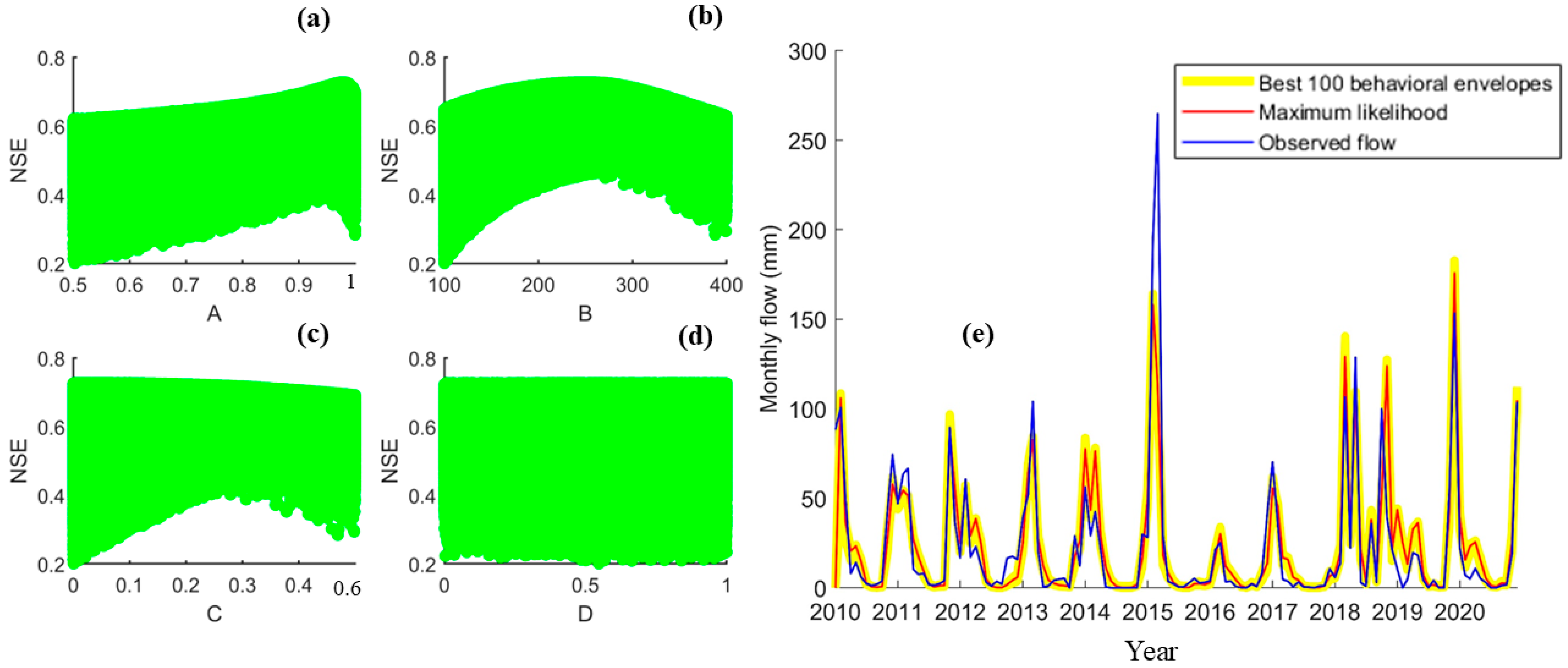
To investigate model sensitivity to the parameters, the multi-dimensional space (${\theta }_i,{NSE}_i)$ from one million simulations was projected on different planes, as seen in Figure 4a–c, Figure 5a–d, and Figure 6a–e, where the y-axis represents the model efficiency, while the x-axis represents each parameter, and the shapes of these scatter plots indicate the model parameter sensitiveness.

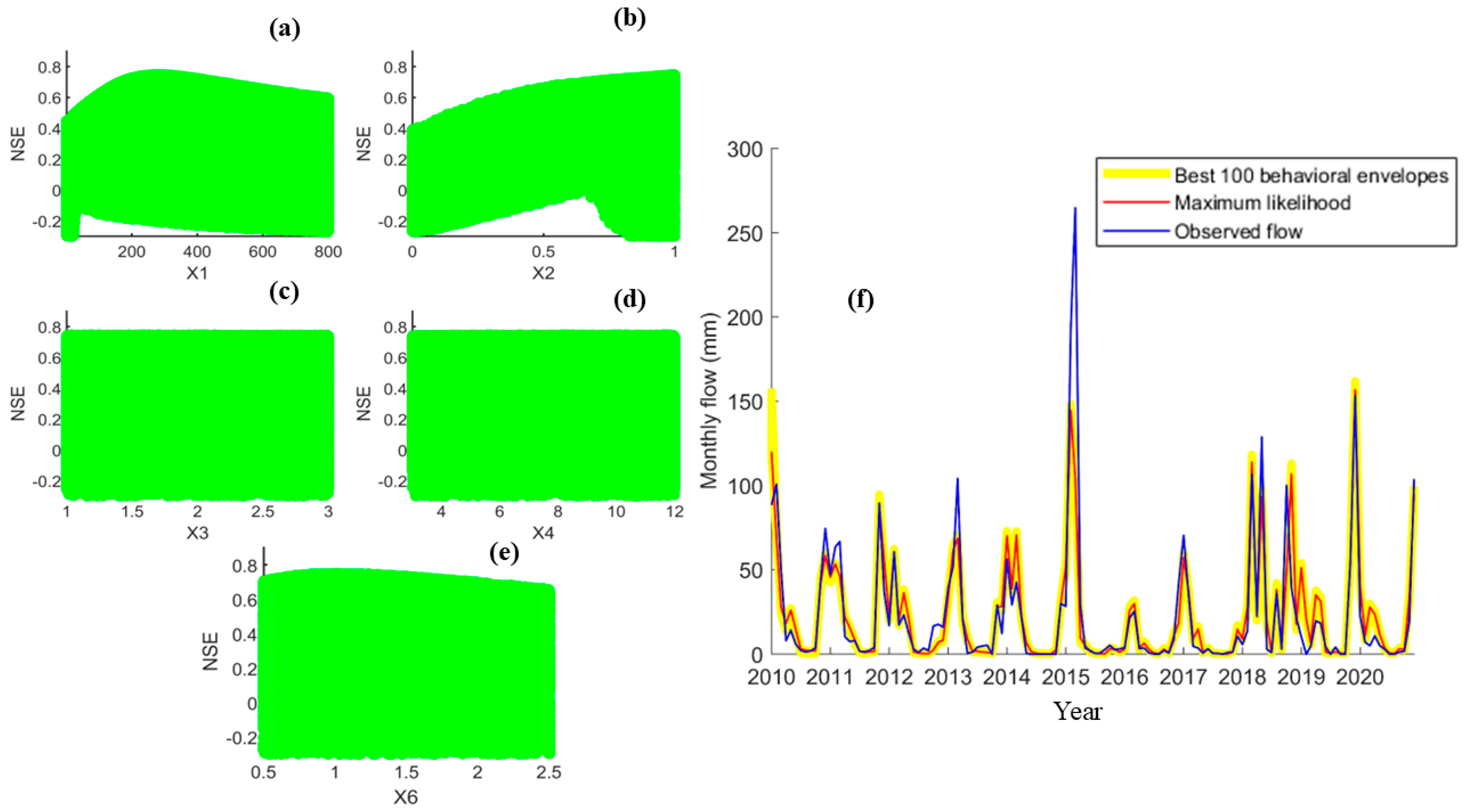
With regard to the GR3M model, the shapes of the scatter plots shown in Figure 4a–c, reveal that the model efficiency is highly sensitive to the water exchange coefficient (${\mathit{X}}_2$), with the highest efficiency obtained for ${\mathit{X}}_2$ = 0.99. For the maximum soil moisture capacity (${\mathit{X}}_1$), the efficiency peaked at 0.75 for ${\mathit{X}}_1$ = 257 mm, after which it declined. In contrast, the routing reservoir capacity (${\mathit{X}}_3$) showed little influence on model performance, with the maximum efficiency occurring at approximately 18 mm and remaining almost unchanged beyond this value.

The ABCD model is highly sensitive to the $\mathit{A}$ parameter, as demonstrated in Figure 5a. The second sensitive parameter is the soil moisture storage maximum water holding capacity ($\mathit{B}$), which has an optimal capacity of 252 mm. Increasing this value beyond 252 mm decreases model efficiency. The groundwater recharge control ($\mathit{C}$) had a minimal impact on model performance, while the groundwater discharge parameter ($\mathit{D}$) increased the model efficiency up to a value of 0.52, after which equifinality was observed.

The analysis carried out for the IHACRES model (Figure 6a) revealed that the maximum soil moisture capacity (${\mathit{X}}_1$), with a value of 280 mm, produced the highest model efficiency. A visual inspection of Figure 6 reveals that the model is very sensitive to the partitioning of effective rainfall into quick and slow flows (${\mathit{X}}_2$), with ${\mathit{X}}_2$ = 0.99 indicating a significant contribution of quick flows to the total streamflow at the catchment’s outlet, coherently with the hydrological description given by the ABCD model. The quick flow recession constant (${\mathit{X}}_3$) exhibited equifinality after 2.5 months, while the slow flow recession constant (${\mathit{X}}_4$) of 9.5 months indicates a prolonged response of the basin’s slow reservoir to rainfall. The evapotranspiration correction factor (${\mathit{X}}_6$), with a value of 1.1, also contributed to the model’s performance.

Finally, as anticipated, the highest 100 equifinal NSE values were selected and the associated parameter sets were retained for the simulation of future streamflows accounting for the variability triggered by the parameters’ uncertainty (Figure 4d,Figure 5e, and Figure 6f).

3.2. Bias-Corrected Future Climate Forcings

Projected changes in rainfall and temperature for the Riu Mannu di Narcao basin are analysed under the RCP 4.5 and RCP 8.5 scenarios. The focus is on the seasonal variability, since they are directly related to freshwater availability and hydrological processes in the region. Figure 7 shows the projected near and far future climate forcings from the GCM-RCM combination under the RCP 4.5 and RCP 8.5 scenarios. The projected monthly mean rainfall from four climate models is displayed in Figure 7a, (Figure 7b) for the near (far) future. Most climate models predict a general decrease in monthly precipitation in both the near and far future under both RCP scenarios, with the exception of July, where an increase in monthly rainfall is foreseen by the majority of models. For August and September, however, the predictions are not coherent, with some models indicating an increase and others a decrease in mean monthly precipitation under both RCP scenarios, reflecting the uncertainty inherent in climate projections. The HadGEM2-ES-RACMO22E model, in particular, predicts significantly different mean monthly temperatures (Figure 7c–f) and precipitation during spring, fall, and winter when compared to observational data and other models.

Far future projections under the RCP8.5 scenario (Figure 7b) indicate the highest decline in monthly mean precipitation occurring during winter (December–February). Given that winter precipitation in Sardinia basins generates the majority of the annual streamflow, while summer and spring rainfall primarily affect evapotranspiration, this reduction could significantly impact future freshwater availability in the Riu Mannu di Narcao basin [5].

In the near future under the RCP4.5 scenario (Figure 7a), winter months, especially December, are expected to bring a significant decrease in monthly means of rainfall, with an average decline of 14 mm. For the RCP8.5 scenario (Figure 7b), in the far future, a considerable decrease in mean monthly rainfall is expected during the winter season, notably in December, with an average reduction of 13 mm compared to the baseline period. In contrast, in the near future, an average increase of 11 mm is expected in mean monthly precipitation during the autumn months, particularly in September and October.

Under the RCP4.5 scenario in the near future (Figure 7c), summer months, particularly June, are projected to experience the largest increase in average minimum temperature by approximately 3 °C, while spring months, especially May, will experience the highest increase in average maximum temperature (Figure 7e) by 3.6 °C. In the far future under the RCP8.5 scenario (Figure 7d,f), for the summer months, particularly August, the largest projected rise is in both minimum and maximum temperatures, with a maximum increase of 4.3 °C.

Under the RCP4.5 scenario, the mean annual rainfall is projected to decrease from 613 mm during the baseline period to 575 mm in the near future and 580 mm in the far future, representing a reduction of 33 mm (5%). For the RCP8.5 scenario, projections indicate that the mean annual precipitation will decrease from 613 mm during the baseline period to 555 mm in the far future (a reduction of 58 mm, or 9%). However, a slight increase in mean annual rainfall is expected in the near future, reaching 623 mm (an increase of 10 mm, approximately 2%).

Under the RCP4.5 scenario, average annual minimum temperature (Tmin) is expected to rise from 11.3 °C during the baseline period to 12.5 °C in the near future and 13.2 °C in the far future, a total increase of 2 °C. Similarly, the average annual maximum temperature (Tmax) is projected to rise from 21.6 °C to 22.8 °C in the near future and 23.5 °C in the far future, also an increase of 2 °C. For the RCP8.5 scenario, the annual average minimum temperature (Tmin) is projected to increase from 11.3 °C in the baseline period to 12.8 °C in the near future and 14.4 °C in the far future (a rise of 3 °C). The annual average maximum temperature (Tmax) is expected to increase from 21.6 °C during the baseline period to 22.9 °C in the near future and 24.6 °C in the far future (a rise of 3 °C).

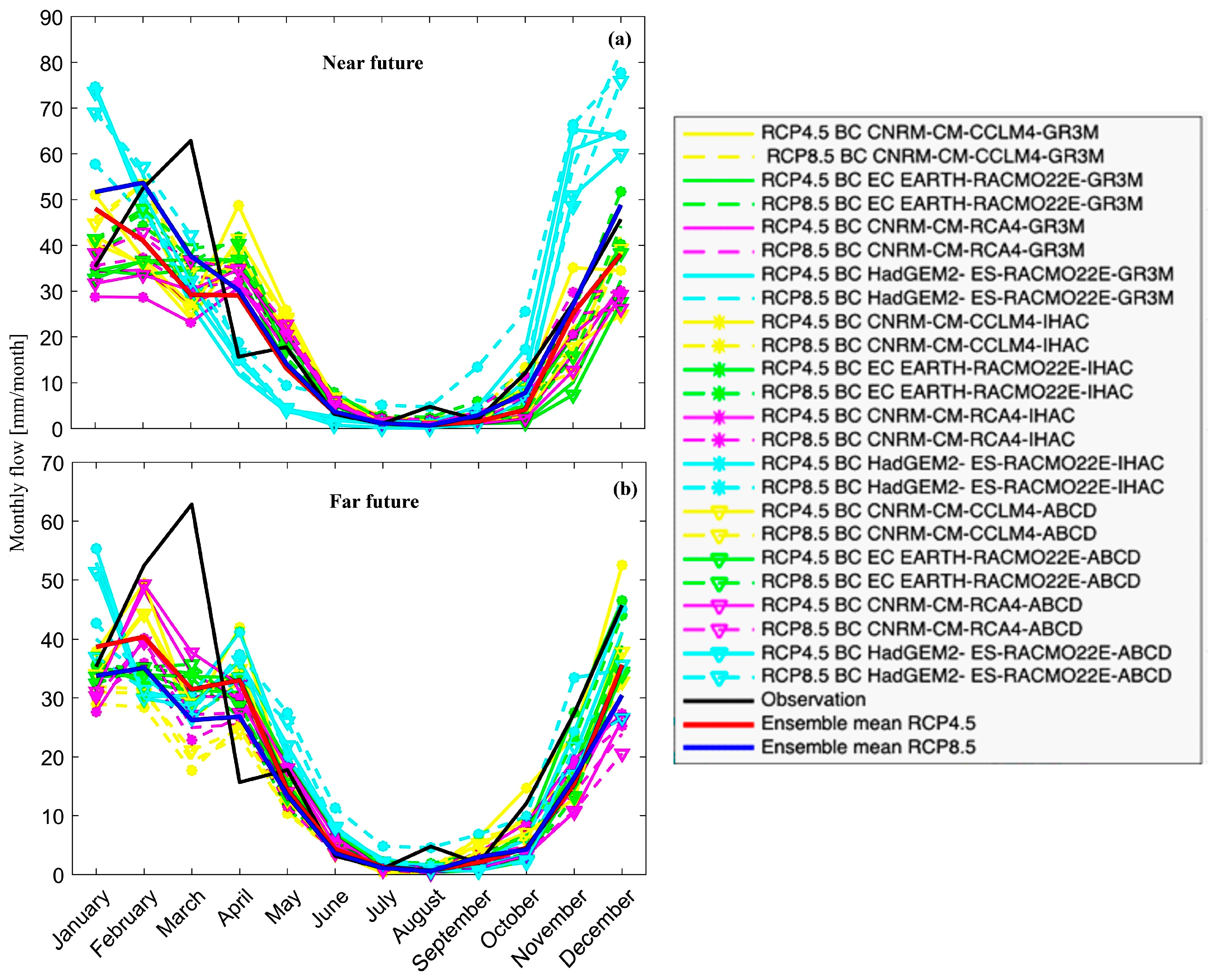
3.3. Projected Future Monthly Streamflows

To simulate future streamflows, bias-corrected future precipitation from the climate models were used as the forcing input into the three hydrological models. At first, parameter sets associated to the optimal Nash and Sutcliffe efficiency (NSE) and then to the 100 best NSE values were used to simulate the future streamflows. The projected future streamflows using the optimal set from the hydrological models (GR3M, IHACRES, and ABCD) forced by four climate models for the near and far future projections under the RCP 4.5 and RCP 8.5 scenarios are shown in Figure 8. The projections show a high consistency across all hydrological models, indicating consistent trends in streamflow predictions despite the different model structures and climate model inputs.

As shown in Figure 8a,b, the ensemble mean monthly streamflows for both scenarios are generally expected to decrease in the near and far future. Streamflow is expected to decline from mid-autumn to early spring (October to March) in the long future forecast under both RCP scenarios, with the largest decline under the RCP8.5 scenario (Figure 8b). This aligns with predictions by Montaldo, N. [5] in the Sardinian basin, which forecast significant reductions in winter runoff due to declines in winter rainfall. Similarly, other studies, including [4,7], have projected reductions in spring and winter streamflows under the RCP8.5 scenario. Overall, the mean monthly streamflow is projected to decrease in the near and far future for both RCP scenarios, primarily due to a decrease in monthly mean precipitation.

To project the future monthly streamflow including also parameter uncertainty, 100 parameter sets for each hydrological model were used to simulate future projections. Thus, we considered the 100 parameter sets associated with the best NSE scores, three hydrological models, four climate models, and two emission scenarios for a total of 2400 streamflow simulated time series. Figure 9 shows monthly streamflows derived from the combination of all hydrological models and climate models in box and whisker plots to visualize future monthly flow variability. As shown in Figure 9a, the majority of the boxplots indicate a general decrease in monthly streamflow, especially from late summer to early spring (August to March). The most pronounced decline is projected to occur by the end of the 21st century under the RCP8.5 scenario. Figure 9b displays the annual streamflow data for the entire year, combining all hydrological and climate model outputs. The median value for the annual streamflow under RCP8.5 is expected to be higher in the near future than the annual streamflow of the near and far future forecasts under the RCP4.5 scenario. However, it was still less than the baseline period. By the end of the 21st century, a lower median streamflow value is forecasted under the RCP8.5 scenario.

Under the RCP4.5 scenario in the near future, a median decrease of 18% in monthly streamflow is predicted (Figure 9a). The largest reduction is expected in September, with streamflow decreasing by over 65% (from 2.1 mm in the baseline to 0.72 mm in the near future). Streamflow also declines by approximately 41% from August to March, ranging between 0.49 mm and 28.5 mm. Notable increases in median monthly flow are expected from mid spring to late summer (April to July). The median annual flow is predicted to decrease from 268 mm in the reference period to 183 mm in the near future, representing a 32% decrease (Figure 9b). These results highlight the need for adaptive water management strategies to mitigate potential water shortages and address the risks associated with climate change.

For the RCP8.5 scenario in the near future (Figure 9a), median monthly flow is predicted to increase in several months, particularly during winter (December to February), as well as in April, May, June, July, and October. The highest increase is projected in May, namely, 159% (from 5.2 mm in the baseline to 13.5 mm in the near future), followed by October (113%) and December (112%). However, August is expected to experience the largest decline at around 64% (from 1.3 mm in the baseline to 0.47 mm in the near future). This variability in streamflow, with both increases and decreases, could exacerbate the frequency of extreme events such as floods and droughts. Despite a projected increase in mean annual rainfall of 10 mm (2%) under the RCP8.5 scenario for the near future, the median annual streamflow under the RCP8.5 scenario is expected to decrease from 268 mm in the baseline period to 202 mm in the near future, representing a 24% decrease (Figure 9b).

In the far future under the RCP4.5 scenario (Figure 9a), the median monthly flow is projected to decrease, with the largest reduction occurring in September (71%) and during late fall to early spring (November to March). The median reduction is approximately 40%, ranging between 6.1 mm to 32 mm. The median annual flow is predicted to decrease by 37% by the end of the century, from 268 mm in the baseline period to 168 mm (i.e., −100 mm) (Figure 9b).

When considering the RCP8.5 scenario (Figure 9a) for the far future, median streamflow is expected to decrease in almost every month, especially from August to March, with a median reduction of around 51%, ranging between 0.4 mm and 25 mm. November is the month with the largest decrease in streamflow, with a 71% reduction. The median annual flow is expected to decrease from 268 mm during the baseline period to 145 mm by the end of the century, representing a significant reduction of 123 mm (46%) (Figure 9b). This significant decline in water availability signals potential future water emergencies exacerbated by climate change, underscoring the need for local water agencies and decision-makers to take early action. These insights could also be relevant to other Mediterranean basins facing similar climate change impacts.

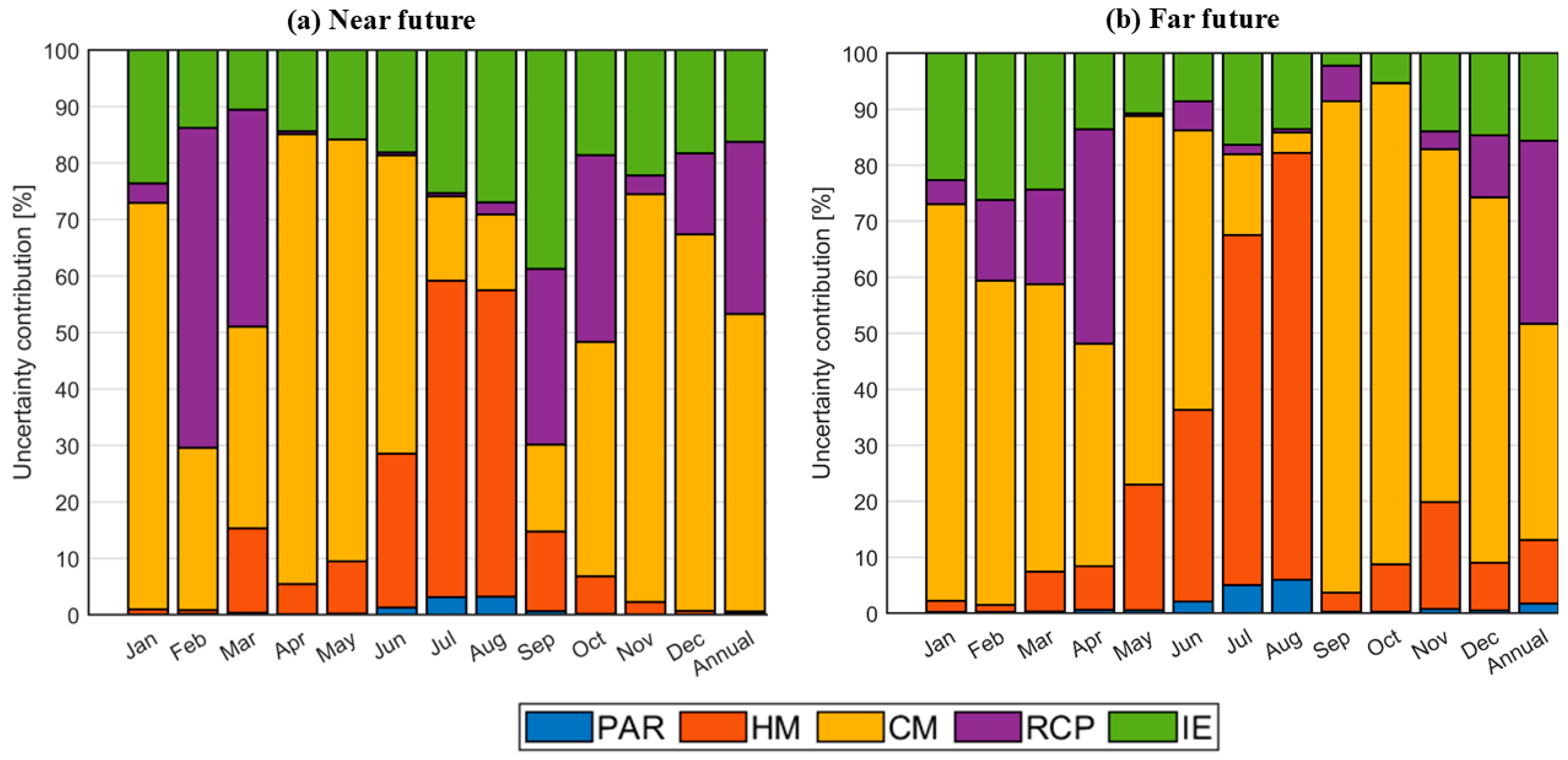
3.4. Quantification of Different Sources of Uncertainty Using ANOVA

The ANOVA approach was used to quantify the contribution of uncertainty from different sources in the projected monthly and annual streamflows throughout the near and far future. Specifically, as discussed in Section 2.5, the ANOVA application was aimed to assess the relative contributions of the main sources, namely, the parameter set (PAR), hydrological model (HM), climate model (CM), climate scenario (RCP), and all possible interaction among two, three, and all main sources. The results are shown in Figure 10a (Figure 10b) and heat maps are shown in

Table 2. Heat map of the near future monthly and annual streamflow projections.

Sources (%)	Jan.	Feb.	Mar.	Apr.	May	Jun.	Jul.	Aug.	Sep.	Oct.	Nov.	Dec.	Average	Annual
PAR	0.09	0.16	0.34	0.12	0.19	1.28	3.12	3.21	0.64	0.17	0.06	0.06	0.79	0.34
HM	0.88	0.66	14.97	5.32	9.28	27.25	56.05	54.28	14.11	6.65	2.19	0.62	16.02	0.22
CM	71.96	28.77	35.71	79.70	74.69	52.86	14.93	13.43	15.37	41.49	72.25	66.71	47.32	52.70
RCP	3.48	56.65	38.44	0.50	0.01	0.50	0.58	2.13	31.16	33.12	3.31	14.34	15.35	30.49
SUM	76.41	86.24	89.46	85.63	84.18	81.89	74.69	73.05	61.27	81.43	77.81	81.74	79.49	83.74
PAR-HM	0.16	0.35	0.89	0.29	0.50	3.03	6.62	6.65	0.98	0.31	0.12	0.12	1.67	0.71
PAR-CM	0.02	0.04	0.05	0.02	0.06	0.46	1.37	1.32	0.24	0.05	0.03	0.01	0.31	0.07
PAR-RCP	0.01	0.01	0.01	0.01	0.01	0.13	0.44	0.42	0.09	0.02	0.00	0.00	0.10	0.02
HM-CM	9.17	3.72	1.38	4.87	6.05	5.17	3.70	1.97	3.78	5.28	5.81	3.37	4.52	5.23
HM-RCP	3.13	1.08	0.04	1.40	1.37	1.33	1.57	1.17	2.18	2.28	2.70	1.56	1.65	2.13
CM-RCP	0.12	5.02	7.69	2.64	3.42	2.92	1.35	6.09	27.83	5.94	5.46	9.26	6.48	1.56
PAR-HM-CM	0.04	0.07	0.11	0.05	0.14	1.00	2.78	2.66	0.56	0.11	0.06	0.03	0.63	0.15
PAR-HM-RCP	0.01	0.02	0.03	0.01	0.01	0.26	0.88	0.86	0.23	0.04	0.01	0.00	0.20	0.03
PAR-CM-RCP	0.02	0.02	0.04	0.01	0.02	0.46	1.53	1.45	0.22	0.02	0.01	0.00	0.32	0.04
HM-CM-RCP	10.87	3.39	0.21	5.05	4.19	2.42	2.03	1.44	2.18	4.45	7.96	3.89	4.01	6.24
PAR-HM-CM-RCP	0.03	0.04	0.07	0.02	0.05	0.94	3.05	2.91	0.43	0.06	0.02	0.01	0.64	0.08
SUM	23.59	13.76	10.54	14.37	15.82	18.11	25.31	26.95	38.73	18.57	22.19	18.26	20.51	16.26

Note: The colors describe the uncertainty contribution of each source in percentage (%): the green color shows low contributions and red color shows high contributions.

(

Table 3. Heat map of the far future monthly and annual streamflow projections.

Sources (%)	Jan.	Feb.	Mar.	Apr.	May	Jun.	Jul.	Aug.	Sep.	Oct.	Nov.	Dec.	Average	Annual
PAR	0.23	0.22	0.31	0.61	0.52	2.08	5.03	5.94	0.25	0.26	0.79	0.48	1.39	1.71
HM	2.01	1.24	7.10	7.76	22.46	34.23	62.49	76.29	3.43	8.47	19.05	8.50	21.09	11.35
CM	70.80	57.94	51.32	39.78	65.84	49.92	14.46	3.64	87.73	85.91	63.02	65.29	54.64	38.62
RCP	4.33	14.40	16.94	38.28	0.44	5.18	1.69	0.60	6.36	0.07	3.16	11.08	8.54	32.69
SUM	77.35	73.80	75.66	86.43	89.26	91.41	83.67	86.47	97.78	94.71	86.02	85.34	85.66	84.37
PAR-HM	0.43	0.47	0.73	1.39	1.26	4.82	10.88	12.63	0.41	0.46	1.45	0.88	2.98	3.48
PAR-CM	0.04	0.03	0.03	0.06	0.01	0.02	0.06	0.03	0.06	0.04	0.07	0.03	0.04	0.07
PAR-RCP	0.00	0.00	0.00	0.00	0.00	0.01	0.01	0.01	0.00	0.00	0.00	0.01	0.00	0.00
HM-CM	0.28	0.59	2.04	0.93	0.65	2.73	4.98	0.64	0.40	1.59	1.33	0.32	1.37	0.38
HM-RCP	0.01	0.02	0.05	0.02	0.05	0.03	0.20	0.10	0.03	0.02	0.11	0.12	0.06	0.01
CM-RCP	21.79	24.98	21.24	10.78	8.70	0.79	0.03	0.01	1.04	3.00	10.55	13.10	9.67	11.46
PAR-HM-CM	0.07	0.05	0.07	0.12	0.02	0.04	0.12	0.07	0.12	0.08	0.14	0.06	0.08	0.13
PAR-HM-RCP	0.00	0.00	0.00	0.00	0.01	0.01	0.03	0.02	0.01	0.00	0.00	0.02	0.01	0.00
PAR-CM-RCP	0.00	0.00	0.00	0.00	0.00	0.00	0.00	0.00	0.00	0.00	0.01	0.00	0.00	0.00
HM-CM-RCP	0.03	0.04	0.16	0.26	0.05	0.13	0.03	0.01	0.13	0.08	0.30	0.12	0.11	0.09
PAR-HM-CM-RCP	0.01	0.01	0.00	0.01	0.00	0.01	0.00	0.00	0.00	0.01	0.01	0.01	0.01	0.01
SUM	22.65	26.20	24.34	13.57	10.74	8.59	16.33	13.53	2.22	5.29	13.98	14.66	14.34	15.63

Note: The colors describe the uncertainty contribution of each source in percentage (%): the green color shows low contributions and red color shows high contributions.

) for the near (far) future.

Overall, the four main effects (PAR, HM, CM, and RCP) account for the larger uncertainty in monthly and annual streamflows. In the near future (Figure 10a and Table 2), the total variance explained by the four main effects in monthly streamflow varies between 61.27% and 89.46% (with an average value of 79.49%), while for the annual streamflow, the contribution from the main effects is 83.74%. Focusing on the far future (Figure 10b and Table 3), the four main effects account on average for 85.79% of the monthly streamflow (varying from 73.8% to 97.78% from month to month) and for 84.37% of the annual streamflow.

In the near future monthly streamflow projection, the GCM-RCM coupling (CM effect) was the single source of the greatest amount of uncertainty, accounting for 13.43–79.70% (average value: 47.32%). This was followed by the hydrological model (HM), which contributed 0.62–56.05% (average value: 16.02%), the RCP scenario, which contributed 0.01–56.65% (average value: 15.35%), and the parameter set (PAR), which contributed 0.06–3.1% (average value: 0.79%). Additionally, as a single source, the GCM-RCM coupling accounts for 52.7% of the uncertainty in the near future annual streamflow, followed by the RCP scenario (30.49%), parameter set (0.34%), and hydrological model (0.22%).

The results of the uncertainty analysis are consistent with those of some earlier research. Climate model variability (GCM-RCM coupling) is the most dominant source of uncertainty in streamflow projections [14,16,27,29]. The results also align with prior research that identified the hydrological model, RCP scenarios, and parameters as significant contributors to the overall uncertainty in streamflow predictions under climate change [13,14,16,28,41,42]. On the other hand, Chen, C. [18] found that model parameter uncertainty is low and may be ignored when making future streamflow projections. Differences in input data, projected values, uncertainty quantification techniques, the type of projected variables (e.g., low or high flow), future periods (near or far futures), and landscape characteristics made it impossible to make direct comparisons with earlier studies. The uncertainty proportion also varied [16,43].

Again, GCM-RCM coupling is the largest single contributor in the far future monthly streamflow projection, accounting for 3.64–87.73% (average value: 54.64%), followed by the hydrological model (1.24–76.29%; average value: 21.09%), the RCP scenario (0.07–38.28%; average value: 8.54%), and the parameter set (0.22–5.9%; average value: 1.39%). Furthermore, GCM-RCM coupling accounts for 38.62% of the uncertainty in the far future annual streamflow, followed by the RCP scenario (32.69%), the hydrological model (11.35%), and the parameter set (1.71%).

The interaction effects (IEs), which are the total of the eleven interaction effects’ uncertainties, account for 10.54–38.73% (average: 20.51%) of the monthly streamflow in the near future (Figure 10a and Table 2). The climate model and RCP interaction (CM-RCP) is the interaction effect that provides the most uncertainty (on average 6.48%) to the monthly streamflow in the near future. HM-CM comes in second with an average of 4.52%, HM-CM-RCP with an average of 4.01%, PAR-HM with an average of 1.67%, and HM-RCP with an average of 1.65%. Interaction effects (IEs) contribute for 16.26% of the annual predicted streamflow in the near future. The largest contributor to uncertainty among the interaction effects is HM-CM-RCP, which accounts for 6.24%. HM-CM, HM-RCP, and CM-RCP follow with 5.25%, 2.13%, and 1.56%, respectively. These results align with prior research that identified interaction effects as significant contributors to the overall uncertainty (14–28%) in streamflow predictions under climate change [16,18].

The interaction effects (IEs) in the far future (Figure 10b and Table 3) monthly streamflow contribute 2.22–26.20% (average value: 14.34%). The interaction effects that contribute the most uncertainty are the climate model and RCP interaction (CM-RCP) (on average 9.67%), followed by PAR-HM (on average 2.98%) and HM-CM (on average 1.37%). The contributions of the other interaction effects are insignificant. The interaction effects (IEs) in the far future prediction account for 15.65% of the annual predicted streamflow. The interaction effects that generate the most uncertainty are CM-RCP (11.46%) and PAR-HM (3.48%). The other IEs are making very little contribution.

In summary, the amount of uncertainty changes from month to month. Climate inputs (GCM-RCM coupling and RCP scenario) were the main contributors to the uncertainty in projected streamflow during the winter, fall, and spring months. In contrast, the hydrological model (HM), model parameters (PAR), and their interaction (PAR-HM) were the main contributors to the streamflow uncertainty during the summer months, especially in July and August [13].

Considering the far future scenarios, the uncertainty contribution by the hydrological model, the climate model (GCM-RCM coupling), and the parameter set in the predicted monthly streamflow increased, whereas the uncertainty contribution by the RCP scenario dropped. When considering the yearly streamflow as a single source, the uncertainty resulting from the hydrological model, RCP scenario, and parameter set rose with increasing time scale, while the climatic model’s contribution dropped. As the time scale grew, the interaction effects’ (IEs’) contributions to the uncertainty in the monthly and annual estimated streamflow were reduced.

These findings are consistent with previous studies, highlighting the significant role of GCM-RCM coupling, hydrological model structures, RCP scenarios, and parameter uncertainty in the uncertainty quantification [28,29]. The results emphasize that climate model variability remains the largest source of uncertainty in hydrological projections, while the hydrological model structure, RCP scenario, and parameter uncertainty also play significant roles in the uncertainty quantification. These findings provide valuable insights for improving hydrological model selection, parameter calibration, and climate scenario assessment, ultimately enhancing the robustness of hydrological projections under future climate conditions.

3.5. Implications and Limitations

For enhanced reliability, several additional investigations are needed. Due to a shortage of available data, this study only calibrated the hydrological models across 11 years, from 2010 to 2020. Compared to other research on climate change, this simulation study is still short, which means that it depicts biased climatic conditions [17]. Our findings should take this limitation into consideration. Due to the lack of observed data in the study basin, the streamflow utilized in this study was reconstructed, as described in the study area. We also found that the reconstructed flow for the year 2015 (Figure 4d, Figure 5e, and Figure 6f) and for March (Figure 8) had bias, which decreased the NSE metric. Therefore, it is recommended that the hydrological models be calibrated using observed streamflow data. Due to lack of long-term historical time series data and because of its simplicity and robustness demonstrated in previous studies, we used the linear scaling bias correction method [44]. This approach works well when mean monthly and annual data are available. It is advised that comparative bias correction techniques be used in future research because the selection of bias correction techniques has a significant influence on the hydrological process [45].

We have further notes for research in the future. This work assessed four uncertainty sources, the hydrological model, the model parameters, the RCP scenarios, and the GCM-RCM coupling, as reflected in the uncertainty quantification. However, the uncertainty resulting from internal climate variability should be considered for improved streamflow projections in the future. We only used the NSE performance metric to select the best 100 parameter sets; however, it is advised to employ multiple performance metrics to evaluate parameter sets.

4. Conclusions

Sardinia, located in the Mediterranean Sea, has historically faced prolonged droughts, and future climate change is expected to further intensify both their frequency and severity. The predicted decline in mean annual precipitation, along with increased surface temperatures and reduced streamflow, present significant threats to the region’s freshwater availability and ecosystem services. Accurate projections of these changes at the local scale (basin level) are essential for developing effective adaptation strategies.

This study aimed to project future streamflows over two periods (near and far future) in Sardinia’s Riu Mannu di Narcao basin by addressing the uncertainties that arise in streamflow predictions under climate change. We considered four primary sources of uncertainty: GCM-RCM coupling, the hydrological model structure, parameters, and RCP scenarios. To quantify these uncertainties, we used the analysis of variance (ANOVA) method. Three conceptual and lumped hydrological models (GR3M, ABCD and IHACRES) were chosen for their effectiveness in simulating historical streamflow and other hydrological components, while the climate models, as suggested by Mascaro, G. [30], were selected based on their accuracy in replicating Sardinia’s historical rainfall and temperature. Bias correction of the climate models was carried out using the linear scaling (LS) method for the Riu Mannu di Narcao watershed.

Future precipitation and temperature projections from the four bias-corrected climate models were used to drive the three hydrological models, accounting for parametric uncertainty. The worst-case future projections indicate an annual decrease in precipitation (−58 mm, i.e., −9%), increases in both the minimum and maximum temperatures (or +3 °C on average), and a significant reduction in streamflow (−123 mm, or 46% less of the median) by the end of the twenty-first century. These findings show that warmer and drier climate scenarios are anticipated for the research area, along with a decrease in the amount of freshwater availability.

Notably, under both RCP scenarios, monthly streamflow is projected to decrease in the near and far future, particularly during the winter months (December–February), raising serious concerns about water resource depletion. However, under the RCP8.5 scenario, a short-term increase in streamflow is expected in the near future. Local water agencies and policymakers must develop adaptation strategies to mitigate the risks of future water shortages and extreme events, such as droughts and floods, exacerbated by climate change.

The uncertainty analysis highlighted that, as a single source, GCM-RCM coupling contributes the most uncertainty 47.32% (54.64%) to the total monthly streamflow prediction in the near (far) future projections uncertainties, followed by the structure of the hydrological model at 16.02% (21.09%), RCP scenarios at 15.35% (8.54%), and parameter uncertainties at 0.79% (1.39%).

This study quantified the main sources of uncertainty in monthly streamflow projections for the Riu Mannu di Narcao basin, showing that GCM-RCM coupling and the hydrological model structure are the dominant contributors. These insights highlight the importance of using multiple climate and hydrological models to guide robust water resource planning in Mediterranean basins. Despite data limitations, this work provides a valuable basis for future studies to refine bias correction methods, expands model ensembles, and accounts for internal climate variability to reduce the predictive uncertainty further.