SPEI Drought Forecasting in Central Mexico

Abstract

This study compares three Standardized Precipitation and Evapotranspiration Index (SPEI) prediction models at different time scales: (1) Kalman filter with exogenous variables (DKF-ARX-Pt, FK), (2) gated recurrent unit (GRU), and (3) autoregressive neural networks with external input (NARX). Using observed data from meteorological stations in the State of Mexico and Mexico City, considering performance metrics, such as mean absolute error (MAE), mean square error (MSE), root mean square error (RMSE), coefficient of determination (R²), Nash–Sutcliffe efficiency coefficient (NSE) and Kling–Gupta efficiency (KGE). The results indicate that the FK model with exogenous variables is the most accurate model for SPEI prediction at different time scales, standing out in terms of stability and low variance in prediction error. GRU networks showed acceptable performance on long time scales (SPEI12 and SPEI24), but with lower stability on short scales. In contrast, NARX presented the worst performance, with high errors and negative efficiency coefficients at several time scales. Models based on Kalman filters can be key tools to improve drought mitigation strategies in vulnerable regions, as it has an improved average predictive accuracy by reducing the MAE by up to 68% and achieving higher consistency in KGE values at longer time scales (SPEI12 and SPEI24).

1. Introduction

Droughts are among the most devastating climatic phenomena for human societies and ecosystems, due to their direct impact on water availability, food security, public health, and economic development. In the context of climate change, an increase in the frequency, duration, and intensity of these events has been observed, particularly in regions of high population density such as the State of Mexico and Mexico City, where pressure on water resources is intensifying [1].

Drought monitoring and forecasting require accurate indicators that are adaptable to different climatic contexts. In this sense, the Standardized Precipitation Evapotranspiration Index (SPEI) has gained relevance due to its capacity to integrate precipitation and potential evapotranspiration (PET), allowing a more comprehensive evaluation of the water balance and its temporal evolution. Unlike other indices such as the SPI, the SPEI allows for the characterization of different types of droughts—meteorological, agricultural, and hydrological—through variable time scales, making it a key tool for water resources planning and management [2,3,4].

In Mexico, several studies have demonstrated the usefulness of SPEI for the retrospective analysis of drought events and its application in the design of public policies. However, its use as a target variable in predictive models still represents an area of scientific development with great potential. Statistical models such as ARIMA, and more recent approaches based on artificial intelligence, such as artificial neural networks (ANNs) and support vector machines (SVMs), have been successfully applied in SPEI prediction, showing higher accuracy in scenarios of high climate complexity [5].

Recent studies have expanded the application of machine learning for drought forecasting. Farzin et al. [6] developed a hybrid of the Bi-directional Long Short-Term Model (BLSTM) and the Harris Hawk Optimization (HHO) model that significantly improved groundwater table predictions in semi-arid regions of Iran. Achite et al. [7] applied an Adaptive Neuro-Fuzzy Inference System (ANFIS) optimized by the Water Cycle Algorithm (WCA) in a hybrid model to forecast hydrological drought in Algeria, achieving higher precision than conventional neuro-fuzzy models. Similarly, Alkubaisi et al. [8] compared a Multilayer Perceptron (MLP) and Long Short-Term Memory (LSTM) architectures for SPEI forecasting in Iraq, finding that shallow models can sometimes outperform deeper networks, emphasizing the importance of model simplicity in short-horizon forecasting. These studies highlight the growing role of soft computing and deep learning techniques in drought modeling and support the need for comparative evaluations across different model types and climatic settings.

Other researchers focus on recent runoff forecasting advances utilizing empirical mode decomposition (EMD) variants integrated with deep learning. For instance, Huang et al. [9] applied an Ensemble Empirical Mode Decomposition (EEMD) method and the Long Short-Term Memory (LSTM) model to forecast daily runoff in southern China’s paddy fields with deep learning combinations to model rainfall–runoff dynamics, while Aviles et al. [10] employed Bayesian network-based models coupled with copula functions for probabilistic drought forecasting in an Andean river basin. These methodological advances reflect the increasing need for tools that balance interpretability, computational cost, and predictive robustness, especially in data-scarce environments.

Forecasting SPEI values using these techniques could substantially improve early warning systems, facilitating informed decision making in sectors such as agriculture, urban water management, and civil protection. In addition, the ability of these models to use accessible meteorological variables such as maximum and minimum temperature and precipitation make them viable and scalable tools for local management [11].

In the search for more accurate methodologies for drought prediction, advanced models such as artificial neural networks (ANNs), Kalman filters, and their variants with exogenous variables have been developed. These approaches not only allow the estimation of current conditions but also enable the prediction of drought behavior through time series. Models based on the Kalman filter with exogenous variables (DKF-ARX-Pt) have proven to be effective in integrating additional climatic information, such as precipitation and temperatures, improving forecast accuracy [12]. Similarly, recurrent neural networks such as GRU and NARX models have shown their ability to identify nonlinear patterns in time series, which is fundamental in modeling extreme weather events [13,14,15,16].

The objective of this work is to develop and evaluate forecast models for SPEI in the region of the State of Mexico and Mexico City, using advanced machine learning techniques and statistical methods, to generate reliable predictions at different time horizons. The aim is to contribute to the construction of scientific tools to mitigate the adverse effects of droughts and strengthen climate resilience in highly vulnerable urban and peri-urban areas.

2. Materials and Methods

2.1. Description of the Study Area

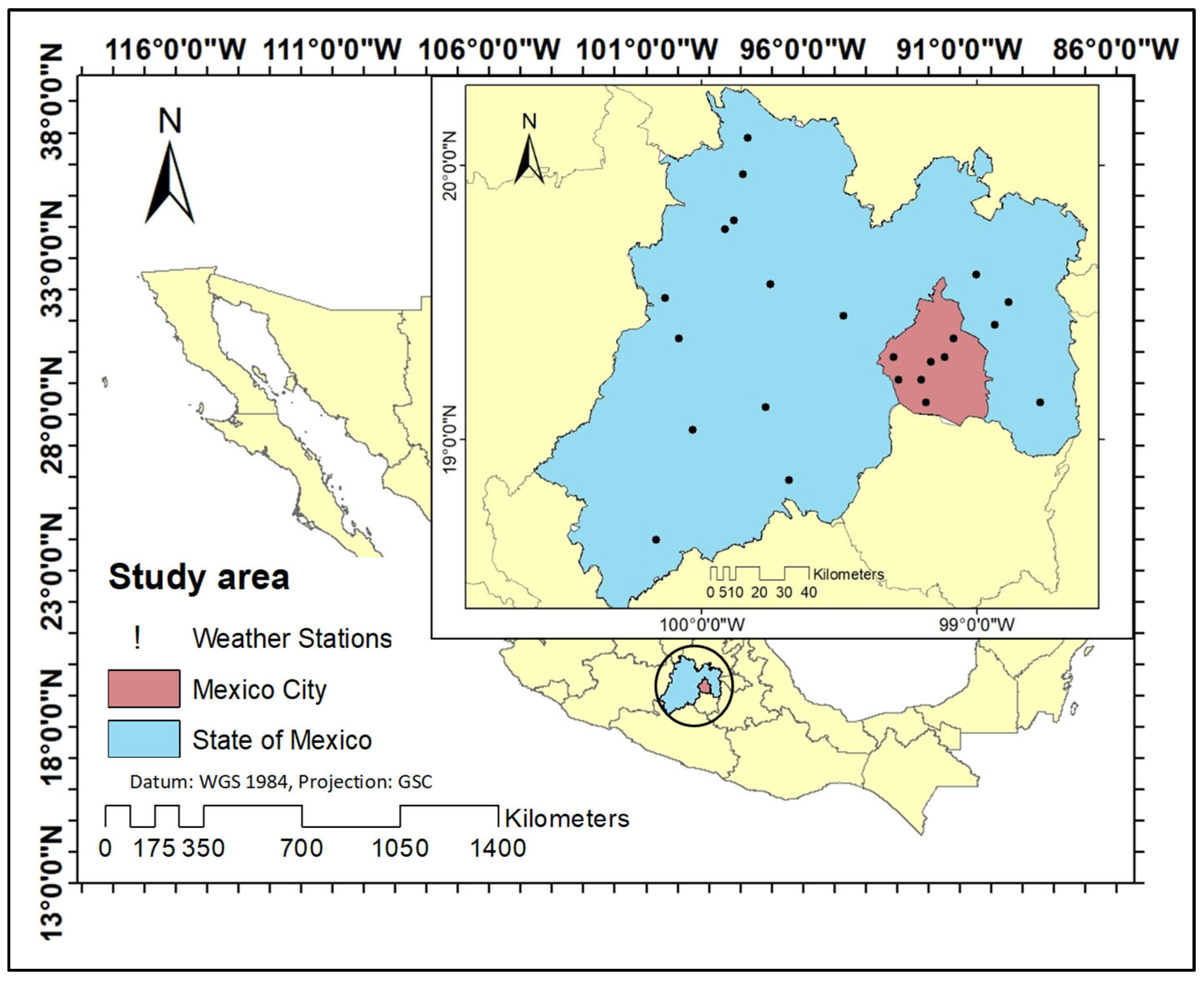
In recent years, there has been an urban growth reflected in the development of new population settlements and civil work developments. According to the last population census conducted by INEGI, the State of Mexico has an area of 22,351.8 km², which represents 1.1% of Mexico’s surface area; however, it is the most populated state with 16,992,418 inhabitants;.Mexico City (CdMx) has an area of 1494.3 km² which represents 0.1% of the country’s surface; Mexico City has 9,209,944 inhabitants. The study area is located between 2250 and 2750 m above sea level; the predominant climate is dry temperate, with an average annual temperature of 15.9 °C and an average annual rainfall of 686 mm; a climate known as sub-humid temperate covers all of the State of Mexico and Mexico City [17].

2.2. Climatological Data

The analysis of 23 meteorological stations across the area of interest over a 42-year period (January 1981 to December 2023) provides a robust dataset for understanding regional climatic trends (Figure 1). Notably, the continued operation of 59% of these stations underscores the challenges of maintaining long-term observational networks. To address gaps and ensure comprehensive data, the geographic coordinates of each station were employed to recover supplementary climatic data via the Climate Engine platform (http://ClimateEngine.org (accessed on 9 September 2024)) [18].

The CHIRPS database was selected due to its capacity to provide precipitation data on daily, pentad, and monthly scales, offering critical granularity. Similarly, the DAYMET database contributed valuable daily and monthly data, complementing the CHIRPS dataset. This dual approach ensures greater reliability in climatic trend analysis, particularly for variables such as precipitation and temperature.

The comparative validation of CHIRPS and DAYMET datasets using observed data from station 15,170 in Chapingo is a critical step in assessing data reliability. The results are highly encouraging, with coefficients of determination (R²) of 0.8921 for precipitation, 0.9974 for maximum temperature, and 0.9824 for minimum temperature. These high R² values indicate strong correlations, affirming the datasets’ suitability for climatological analysis [19].

Although CHIRPS and DAYMET are widely used gridded climate datasets in drought and hydrological research, they are not without limitations. CHIRPS combines satellite-derived precipitation estimates with station-based observations, which can introduce biases in areas with sparse ground data or complex topography [20]. Spatial interpolation errors and temporal inconsistencies have been reported in mountainous regions such as central Mexico [21]. DAYMET, which provides high-resolution daily temperature and precipitation estimates based on interpolation from meteorological stations, can also exhibit elevation-related biases and smoothing effects that limit its accuracy in terrain-diverse or urbanized environments [22]. Several validation studies have shown that CHIRPS generally performs well for regional precipitation analysis, especially at monthly scales, but it may underestimate extreme rainfall events [23]. Similarly, DAYMET has demonstrated acceptable performance for temperature estimation in North America but is sensitive to local station density and quality [22]. In our study, while CHIRPS and DAYMET provided consistent coverage for the State of Mexico and Mexico City, minor discrepancies were observed between gridded and in situ values, particularly under extreme climatic conditions. These uncertainties should be acknowledged when interpreting model outputs and assessing generalizability beyond the calibration domain.

2.3. CHIRPS Satellite Information

The CHIRPS algorithm combines three data sources: (a) the CHPclim precipitation climatology, a 0.05° global climatology based on data from stations, satellite observations, elevation, and coordinates [20]; (b) satellite estimates of infrared thermal precipitation (IRP); and (c) in situ rain gauge measurements. CHPclim differs by using long-term satellite averages to improve its accuracy, especially in mountainous regions [24]. Combining CHIRP with station data uses the estimated correlation between a pixel’s precipitation and nearby stations [25].

Data merging is performed on 5-day (pentad) and monthly scales, adjusting the pentads so that their sum matches the monthly total. A daily version is generated from this data. Preliminary CHIRPS is published 2 days after a pentad, and the final version is in the third week of the following month.

2.4. DAYMET Satellite Data

The Daily Surface Weather Data provides continuous, gridded estimates of daily weather variables by interpolation and statistical modeling. It includes minimum and maximum temperature, precipitation, vapor pressure, shortwave radiation, snow water equivalent, and day length, on a 1 km² grid for North America and Hawaii since 1980, and Puerto Rico since 1950.

The Daymet method estimates meteorological parameters at instrumented sites by interpolation and extrapolation, using weighted data from nearby stations. In the Daymet V4 version, station selection is optimized by eliminating the iterative density calculation, defining instead a fixed search radius based on pre-computed distances. Two workflows generate variables: one for daily temperature and one for precipitation [22].

2.5. Standardized Precipitation Evapotranspiration Index (SPEI)

The Standardized Precipitation Evapotranspiration Index (SPEI) is an extension of the SPI that incorporates both precipitation and potential evapotranspiration (PET) to evaluate drought, considering the impact of temperature increase on water demand.

The SPEI is calculated using the water balance (Di = P-ETo) at different time scales (1, 3, 6, 12, and 24 months). Unlike the SPI, which only uses precipitation, the SPEI provides a more accurate measure of drought severity by including atmospheric evaporative demand.

Initially, the Thornthwaite equation [26] was proposed to estimate evapotranspiration due to its simplicity, but more accurate methods such as the FAO-56 Penman–Monteith equation [27] are preferable if sufficient data are available. Failing this, the Hargreaves equation, which was used in this study, is recommended.

The SPEI calculation was performed in RStudio^® with the SPEI.R software version 1.8.1 [28], using data on the precipitation, minimum and maximum temperature, and latitude of the study site. The values obtained were analyzed according to the classification of McKee, Doesken, and Kleist [29] to identify the evolution of droughts, their intensity, duration, and dates of onset and termination (see

Table 1. SPEI categories and classification [29].

Index Value	Category
>2.00	Extremely humid
1.50 to 1.99	Very humid
1.00 to 1.49	Moderately humid
−0.99 to 0.99	Near normal
−1.00 to −1.49	Moderately dry
−1.50 to −1.99	Very dry
<−2.00	Extremely dry

).

2.6. Selection of Representative Weather Stations

For the identification of representative weather stations in the context of climate change and drought assessment, a quantitative approach was implemented based on the nonparametric Mann–Kendall statistical test [30,31], widely used for the detection of monotonic trends in climatic time series [32,33].

Three fundamental climatic variables were analyzed, namely, monthly cumulative precipitation (PCP), maximum temperature (TMAX) and minimum temperature (TMIN), using data from 381 meteorological stations. Z-statistic values were calculated for each variable at each station. Significant trends were considered to be those whose absolute value of the Z statistic was greater than or equal to 1.96 (95% confidence level).

The stations were classified into three levels of representativeness:

• Highly representative: stations with significant trends in two or more variables.
• Moderately representative: stations with only one significant variable.
• Unrepresentative: stations with no significant trends.

This classification approach has been used in similar studies to identify key stations for climate change monitoring. For example, Ahmad et al. [34] applied criteria based on the number of variables with significant trend to select critical stations in a South Asian basin. Similarly, Kousari et al. [35] classified stations according to the magnitude and significance of detected changes in temperature and precipitation, which allowed identifying control points for vulnerability analysis. In addition, Gong et al. [36] proposed a regional pattern recognition methodology that included the hierarchization of stations by their degree of climate response, which is compatible with the classification used in this study.

Additionally, a climate pattern was assigned to each station based on the combination of detected trends, following criteria similar to those employed by recent studies on the classification of local climate responses [2,36,37].

• Dry and warm: significant decrease in precipitation and increase in TMAX or TMIN.
• Dry and cold: decrease in precipitation and decrease in temperature.
• Strong warming: significant increase in TMAX or TMIN without relevant changes in precipitation.
• Climatic stability: no significant trends.

This methodology not only allows an objective and reproducible selection of stations for the monitoring and analysis of climate change but also facilitates the zoning of areas with homogeneous climate behavior, which is essential for regional drought studies (SPEI) and planning of adaptation measures (

Table 2. An example of the classification of stations with their respective Z-values and assigned weather patterns.

ID	Name	PCP	TMAX	TMIN	Classification	Weather Pattern
9002	Ajusco	−1.53	12.39	3.55	Moderately Representative	High temperature
9004	Calvario 61	−1.07	11.86	3.73	Moderately Representative	High temperature
9014	Santa Úrsula Coapa	−1.18	4.51	3.97	Moderately Representative	High temperature
9019	Desierto De Los Leones	−2.35	9.95	0.79	Highly Representative	Dry and warm
9022	El Guarda	−1.67	14.1	1.22	Moderately Representative	High temperature
9026	Morelos 77	0.2	0.64	2.61	Moderately Representative	Mixed change
9067	Monte Alegre	−2.23	7.42	−4.04	Highly Representative	Dry and warm
15001	Acambay	−1.01	6	9.11	Moderately Representative	High temperature
15002	Aculco (Smn)	−1.56	10.44	5.45	Moderately Representative	High temperature
15006	Amatepec	−1.76	8.51	−6.14	Highly Representative	High temperature
15007	Amecameca De Juárez	−1.38	8.64	3.67	Moderately Representative	High temperature
15009	Atlacomulco	−2.23	7.74	6.29	Highly Representative	Dry and warm
15023	Chimalhuacán	0.02	5.5	3.59	Moderately Representative	High temperature
15034	Ixtapan De La Sal	−2.03	9.71	1.96	Highly Representative	Dry and warm
15036	Ixtlahuaca (Smn)	−1.51	8	5.45	Highly Representative	High temperature
15061	Nezahualcóyotl	0.68	1.02	2.04	Moderately Representative	Mixed change
15062	Nevado De Toluca	−2.31	15.35	−1.14	Highly Representative	Dry and warm
15066	Palizada	−2.58	13.07	6.88	Highly Representative	Dry and warm
15118	Temascaltepec	−2.9	9.01	3.49	Highly Representative	Dry and warm
15131	Villa De Allende	−2.53	12.1	3.76	Highly Representative	Dry and warm
15170	Chapingo (Dge)	−0.19	2.35	6.62	Moderately Representative	Humid and warm
15231	Presa Iturbide	−4.04	12.09	6.43	Highly Representative	Dry and warm
15277	San Miguel Tenochtitlan	−2.48	7.43	5.25	Highly Representative	Dry and warm

). Moreover, the approach has been validated in similar research in regions of Mexico and other parts of the world [35,38].

2.7. Drought Forecasting

Anticipating the characteristics of a drought (magnitude, duration, and distribution) is key to mitigating its effects [4]. Accurate forecasting improves water resource management and is based on climatic indicators such as precipitation or specialized indices such as SPI and SPEI.

Mishra & Singh [39] discuss various drought forecasting methodologies, including regression, time series, probabilistic models, artificial neural networks (ANNs), hybrid approaches, and data mining. In recent years, ANNs have stood out for their machine learning capabilities [40], being applied in hydrology to model rainfall–runoff, flow rates, groundwater, and water quality [41]. Their main advantage is to identify nonlinear patterns without the need for predefined mathematical models [42].

The combination of neural networks and Kalman filters has been studied in drought prediction and SPEI calculation. Models such as DKF-ARX-Pt (Kalman filter with exogenous variables such as precipitation and temperature), GRU (gated recurrent unit), and NARX (neural autoregressive networks with external input) have been applied.

2.8. Model Selection

The selection of forecasting models—FK (Kalman filter with exogenous variables), GRU, and NARX—was performed based on a combination of interpretability, computational efficiency, and proven performance in time series forecasting under data-scarce conditions. The Kalman filter (FK) was selected for its low computational cost, probabilistic formulation, and ability to integrate exogenous variables, making it suitable for operational use in regions with variable data quality. GRU was chosen over more complex architectures like LSTM due to its simpler structure and comparable performance, especially on medium- and short-term forecasting horizons, as demonstrated by Alkubaisi et al. [8]. GRUs also train faster and require fewer parameters, which is advantageous when working with monthly climatic series such as the SPEI. The NARX model was included due to its established use in modeling nonlinear dependencies in hydrological and climate time series, supported by prior research [13,14].

Recent hybrid ensemble and decomposition-based models have shown enhanced predictive skill but at the cost of greater complexity and reduced interpretability. For example, hybrid Complementary Ensemble Empirical Mode Decomposition (CEEMD) long short-term memory (LSTM) outperformed single LSTM in SPI forecasting within China [43], and Convolutional Neural Network (CNN)–LSTM and Improved Complete Ensemble Empirical Mode Decomposition with Adaptive Noise (ICEEMDAN)—Northern Goshawk Optimization (NGO)–LSTM hybrids have demonstrated strong results in streamflow and hydrological forecasting at sub-seasonal scales [44,45]. However, deploying such models in practice requires significant infrastructure and expertise. Our study therefore benchmarks three diverse yet pragmatic models spanning statistical, recurrent, and neural paradigms. This approach provides a solid foundation for future work exploring advanced hybrids—such as CNN-GRU, transformer-based ensembles [46], or multi-source architectures [45]—without compromising reproducibility or operational utility.

2.9. Kalman Filter with Exogenous Variables (DKF-ARX-Pt)

The Kalman filter with exogenous variables, known as DKF-ARX-Pt, is an extension of the classical Kalman filter, used to estimate the state of dynamic systems under uncertainty, but incorporating external or exogenous variables that influence the process. Traditionally, the Kalman filter is used in linear systems where a model of the system is known, and the state of the system is estimated as noisy observations are received. However, in complex phenomena such as drought, prediction models must consider not only past observations of the system itself (such as drought indices), but also external factors that affect its evolution, such as precipitation and temperature [12].

The ARX (autoregressive with exogenous input) model is fundamental in the formulation of the DKF-ARX-Pt, since it extends the classical auto-regressive time series model to include inputs from external variables. This model takes the form, Equation (1):

$$y\left(t\right)=\sum _{i=1}^p{a}_{i}y\left(t-i\right)+\sum _{j=1}^q{b}_{j}u\left(t-j\right)+e\left(t\right)$$

(1)

where

• y(t) is the dependent variable (e.g., the drought index such as the SPEI);
• u(t) is the exogenous input (such as precipitation or temperature);
• ai and bj are the autoregressive and exogenous coefficients, respectively;
• e(t) is the model error.

In the context of the Kalman filter, the DKF-ARX-Pt incorporates these exogenous inputs within the state estimation framework, allowing the model to adjust not only based on system observations but also on the influences of external climatic variables.

2.10. Gated Recurring Unit (GRU)

Gated recurrent unit (GRU) is a type of recurrent neural network (RNN) that is highly effective in time series modeling, including the prediction of climate variables such as drought. Introduced by Cho et al. [13], GRUs have been used for problems where long-term dependence and gradient propagation are critical, such as meteorological data analysis and the prediction of climatic phenomena.

Their main advantage over traditional RNNs lies in their ability to mitigate the gradient fading problem, allowing them to capture long-term relationships in temporal data. This is particularly relevant in drought prediction, where current conditions may be influenced by climatic events that occurred months or even years ago [47].

2.11. Autoregressive Neural Networks with External Input (NARX)

Neural autoregressive networks with external input (NARX) have proven to be an effective technique for modeling nonlinear dynamical systems, including drought prediction. Proposed by Lin et al. [14], NARX extend classical autoregressive models by capturing nonlinear relationships between climate variables, differing from traditional approaches such as ARIMA or ARX. In SPEI prediction, they can integrate exogenous variables such as precipitation and temperature to improve accuracy. Hernández-Vásquez et al. [48] applied artificial neural networks in the Sonora River basin, obtaining an average R² of 0.76 in validation, evidencing its predictive capacity.

2.12. Prediction Model Evaluation Metrics

In the evaluation of time series and hydrological models, it is essential to quantify both error magnitudes and goodness-of-fit. The following metrics were used to compare SPEI forecasting models:

• MAE (mean absolute error): Measures average absolute deviation between predictions and observations; less sensitive to outliers than squared metrics [49].
• MSE (mean squared error) and RMSE (root mean squared error): Average squared deviations and their square root; RMSE penalizes larger errors more heavily [50].
• R² (coefficient of determination): Proportion of variance explained by the model, indicating overall fit [51].
• NSE (Nash–Sutcliffe efficiency coefficient): A hydrological standard equivalent to R² for model efficiency; values closer to 1 indicate higher predictive skill [52].
• KGE (Kling–Gupta efficiency): Integrates correlation, bias, and variability into a single metric, offering a balanced evaluation of model performance [53].

This suite of metrics provides a comprehensive view of predictive accuracy and reliability, facilitating the selection of the most appropriate SPEI forecasting approach.

2.13. Model Training and Forecasting

A time-based split was used for model validation: 70% of the data was used for training and 30% for testing, maintaining chronological order to preserve causality and avoid data leakage [54]. For each training example, a rolling window of 36 months was used as input to predict the subsequent SPEI value, with no future data included in the training sequences [55]. All normalization was performed using scaling parameters derived solely from the training data and then applied to the test set to ensure strict separation between training and evaluation processes [56].

This flowchart (Figure 2) helps clarify the sequential structure of the methodology, especially the parallel processing of multiple models (FK, GRU, and NARX) and SPEI time scales. It also highlights the integration of uncertainty analysis and model comparison as essential components of the forecasting framework.

Although the evaluation of predictive accuracy is based on average metrics such as MAE, RMSE, R², NSE, and KGE, model selection also considers computational efficiency, stability across stations and SPEI scales, and the robustness of the predictions under uncertainty.

• Calibration strategy: In order to calibrate and fairly compare the three forecasting approaches (Kalman filter, NARX, and GRU), we split each station’s monthly SPEI series into a training set and a test set, using a 70%/30% chronological split. That is, for each station and each horizon we used the earliest 70% of the data (1981–2018) to fit the model and reserve the last 30% (2019–2023) for out-of-sample evaluation [57].
• Cross-validation: Within the training window we applied a rolling 10-fold cross-validation. At each fold, the model is re-estimated on 80% of the training block and validated on the remaining 20%, sliding forward by one year per fold. Hyperparameters (e.g., GRU cell size, NARX lag order, and process noise in the Kalman filter) were selected to minimize mean squared error in CV.
• Reproducibility: For all random operations (weight initialization in GRU and data shuffling in CV), we fixed a global seed (e.g., np.random.seed [41] and the equivalent in TensorFlow) to ensure that results can be exactly reproduced.
• Final evaluation: Once hyperparameters were fixed, each model was retrained on the entire training period and then ran on the hold-out test set. All performance metrics reported in the results that derive from this test set forecast.

The FK model incorporates uncertainty through stochastic simulations: during forecasting, random process noise was added at each step using a multivariate normal distribution derived from the model’s estimated state covariance matrix [12]. This enabled the generation of a distribution of possible future values and the construction of confidence intervals for 3- and 6-month forecasts [58]. Although this uncertainty mechanism was not implemented in the GRU and NARX models, future work will explore techniques such as Monte Carlo dropout [59] or bootstrap ensembles [60] to quantify prediction uncertainty in deep learning settings.

The absence of formal uncertainty quantification in the GRU and NARX models is acknowledged as a limitation. Incorporating such methods will be essential to improve the reliability of model outputs, especially for operational drought early warning systems and climate risk planning.

The GRU and NARX models were implemented using the Keras API in TensorFlow [61]. Both architectures received input sequences of the previous 36 months of meteorological data (precipitation and maximum and minimum temperature). Each consisted of two recurrent layers—GRU for the GRU model [13] and LSTM for the NARX model [62]—each with 64 units and tanh activation. Droput layers (rate = 0.2) were added after each recurrent layer to reduce overfitting [63]. The output layer used a single neuron with linear activation. Models were trained using the Adam optimizer [64] with a learning rate of 0.001, a batch size of 32, and Mean Squared Error (MSE) loss, for 50 epochs. Hyperparameters were selected based on preliminary convergence and validation performance assessments.

All models and analyses were implemented using Python 3.11 within the PyCharm IDE on a Windows 10 operating system. The following packages and libraries were used:

• TensorFlow 2.15 and Keras 2.15 for deep learning model development (GRU, NARX)
• NumPy 1.24 and Pandas 1.5 for data manipulation
• Scikit-learn 1.2 for metrics and preprocessing
• PyKalman 0.9.5 for Kalman filter implementation
• Matplotlib 3.7 for plotting
• SciPy 1.10 and Statsmodels 0.13 for statistical tests
• OpenPyXL 3.1 for Excel output handling

3. Results

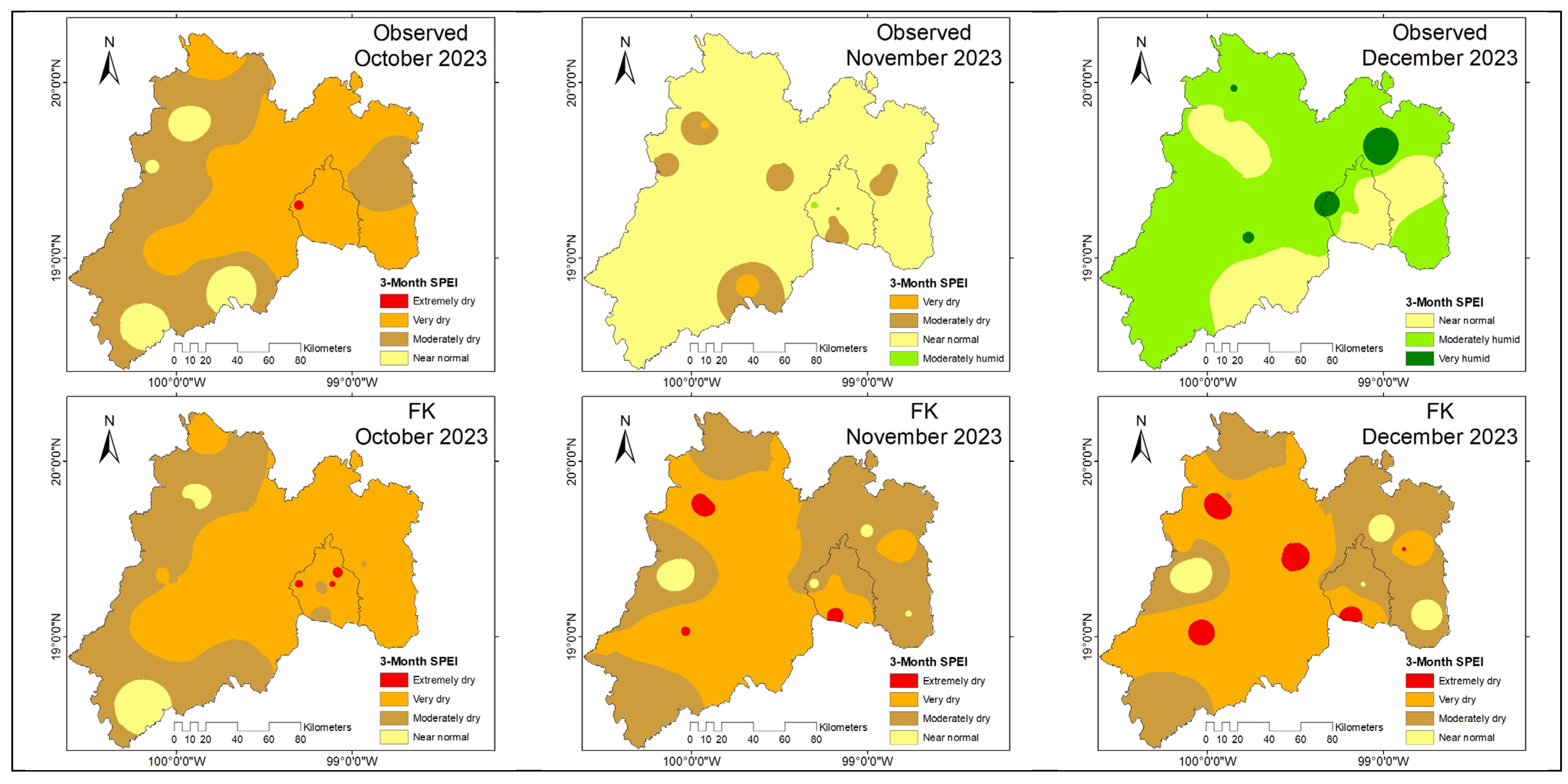
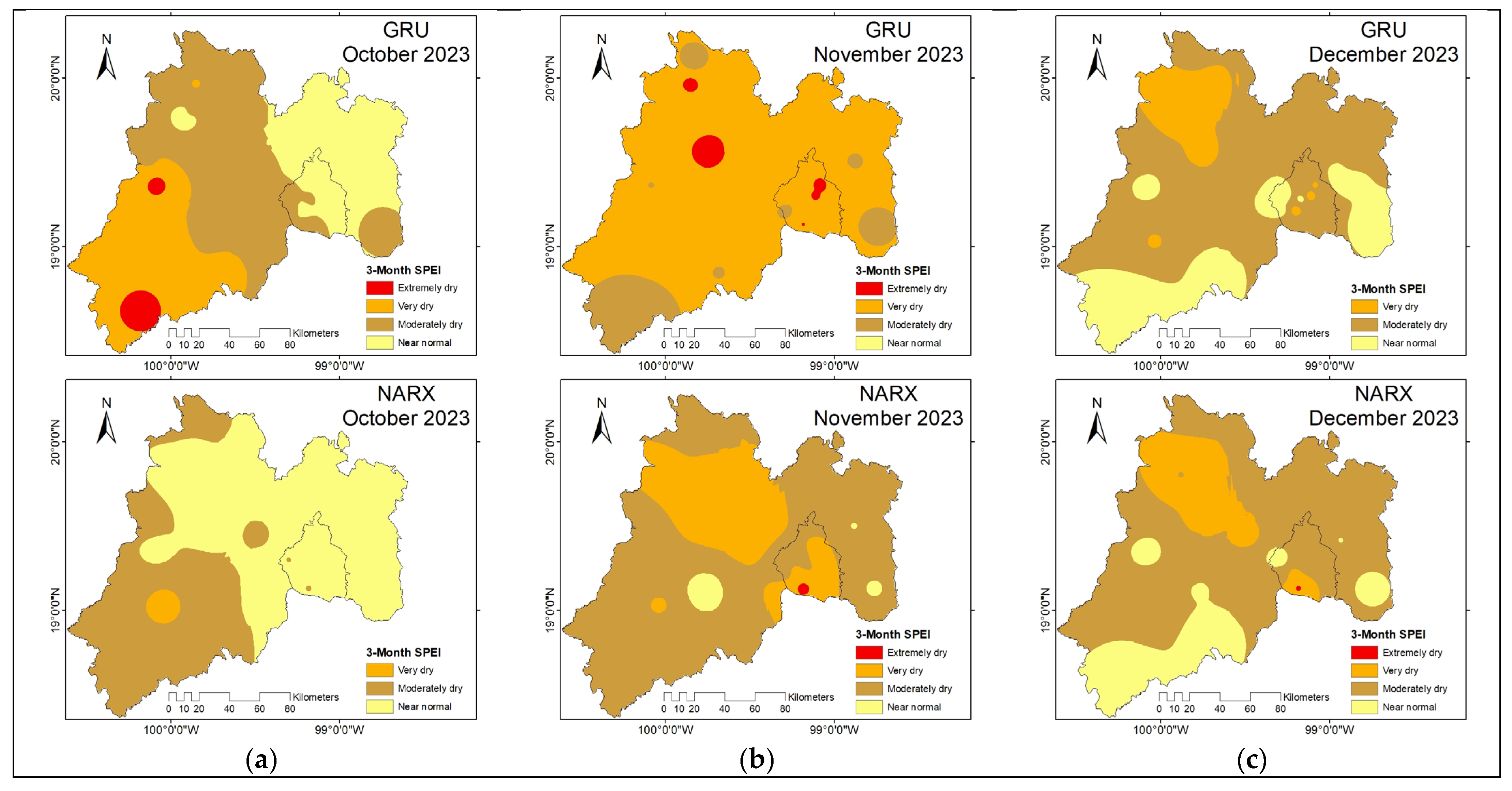
Three methodological approaches were applied to forecast the SPEI in 23 stations in the State of Mexico and Mexico City: the Kalman filter with exogenous variables (FK or DKF-ARX-Pt), autoregressive neural networks with external input (NARX), and gated recurrent unit (GRU).

Table 3. Main parameters used for each forecasting model.

Model	Parameters
FK (DKF-ARX-Pt)	- AR order: 2 - Exogenous order: 2 - Q: estimated from residual variance - R: tuned via cross-validation - Initialization from first 12 months
GRU	- 2 layers with 64 units each - Dropout: 0.2 - Optimizer: Adam - Learning rate: 0.001 - Batch size: 32 - Epochs: 50
NARX (LSTM-based)	- 2 LSTM layers with 64 units each - Dropout: 0.2 - Optimizer: Adam - Learning rate: 0.001 - Batch size: 32 - Epochs: 50 - Input/output lags: 3

summarizes the main parameters used to train each forecasting model. The FK model, based on a deterministic Kalman filter, relies on predefined AR and exogenous orders and requires minimal tuning. In contrast, the GRU and NARX models were optimized using neural architecture with dropout regularization and gradient-based learning.

Among the evaluated models, the Kalman filter (FK or DKF-ARX-Pt) exhibited the lowest computational effort, with training times below one minute per station. In contrast, deep learning models like GRU and NARX required significantly more time due to iterative optimization over 50 epochs (

Table 4. Average training time per model (per station) using Intel Core i7, 16 GB RAM.

Model	Average Training Time (Per Station)
FK (DKF-ARX-Pt)	~0.8 min
GRU	~12 min
NARX	~15 min

).

While NARX obtained the best average values in all performance metrics (

Table 5. Summary of the averages of each metric for the three models.

Model	MAE	RMSE	R2	NSE	KGE
FK	0.117	0.159	0.976	0.976	0.735
GRU	0.101	0.140	0.980	0.980	0.829
NARX	0.098	0.136	0.982	0.982	0.864

), the DKF-ARX-Pt (FK) model demonstrated more consistent behavior across stations and time scales, in addition to requiring less computational effort (Table 4). Despite slightly lower accuracy in average metrics, FK offers a more robust and stable performance across different scenarios. This consistency was observed throughout all stations and SPEI time scales evaluated, making FK particularly suitable for operational forecasting. The GRU model showed competitive performance in some cases but suffered from higher variance and less reliable convergence. NARX, although occasionally reaching higher accuracy for specific stations, lacked general robustness and presented longer training times.

The NARX model was the most accurate in absolute terms, with the lowest MAE and RMSE values and the highest R², NSE, and KGE. This indicates that it was able to reproduce both the general trend and the internal variability of the SPEI series with a high degree of fidelity. GRU also performed outstandingly well, especially at intermediate scales (SPEI3 to SPEI6), where it offered accuracy comparable to NARX with lower computational demands.

As shown in

Table 6. Paired tests (t-test and Wilcoxon) between pairs of models for each metric and horizon (α = 0.05).

Prediction	Metric		Model 1		Model 2		t-Stat	p-Value t-Test	W-Stat	p-Value Wilcoxon
3 months	MAE		FK		NARX		1.23	0.224	1.1	0.27
3 months	MAE		FK		GRU		3.21	0.012	2.45	0.018
3 months	MAE	NARX	GRU	2.87	0.023	2.17	0.031
3 months	RMSE	FK	NARX	1.45	0.165	1.3	0.195
3 months	RMSE	FK	GRU	3.05	0.017	2.3	0.022
3 months	RMSE	NARX	GRU	2.6	0.029	2.05	0.042
3 months	R2	FK	NARX	1.1	0.285	0.95	0.345
3 months	R2	FK	GRU	2.75	0.02	2.2	0.028
3 months	R2	NARX	GRU	3	0.011	2.4	0.015
6 months	MAE	FK	NARX	0.78	0.442	0.68	0.495
6 months	MAE	FK	GRU	1.02	0.321	0.98	0.328
6 months	MAE	NARX	GRU	3.85	0.004	3	0.007
6 months	RMSE	FK	NARX	0.56	0.579	0.45	0.651
6 months	RMSE	FK	GRU	1.02	0.321	0.98	0.328
6 months	RMSE	NARX	GRU	3.85	0.004	3	0.007
6 months	R2	FK	NARX	1.56	0.132	1.4	0.158
6 months	R2	FK	GRU	2.1	0.048	1.95	0.052
6 months	R2	NARX	GRU	2.45	0.031	2.2	0.028

, at the 3-month horizon, the GRU model achieves a significantly lower MAE than the Kalman filter (t (n–1) = 3.21; p = 0.012; Wilcoxon p = 0.018) and a significantly higher RMSE performance against NARX (t = 3.05; p = 0.017; Wilcoxon p = 0.022). GRU also outperforms NARX in R² (t = 3.00; p = 0.011; Wilcoxon p = 0.015). In contrast, the differences between the Kalman filter and NARX at 3 months are not statistically significant (p > 0.05 for MAE, RMSE, and R²).

At the 6-month horizon, only the RMSE comparison between NARX and GRU is significant (t = 3.85; p = 0.004; Wilcoxon p = 0.007), indicating that NARX maintains lower error variability over longer lead times. No other pairwise differences (FK vs. RN or FK vs. GRU) reach significance (all p > 0.05 in MAE, RMSE, and R²), suggesting comparable performance among those models at six months.

Overall, these statistical tests confirm the superiority of GRU for short-term (3 m) SPEI forecasting, while for medium-term (6 m) applications, NARX and the Kalman filter provide equally reliable results.

The FK model presented (Figure 3) the best overall performance in predicting the 3-month SPEI3: low average MAE (~0.10), indicating a small average deviation from the observed values; also low RMSE (~0.13), confirming the model’s consistency in prediction; R² ≈ 0.98, implying that the model explains 98% of the observed variability of SPEI3; NSE ≈ 0.98, which is considered excellent by hydrological standards; KGE ≈ 0.85, a sign that the model adequately reproduces the distribution, skewness and variability of the data. It is the most reliable model for short-term SPEI3 prediction, with high accuracy and robustness.

The GRU model showed moderate performance compared to FK: average MAE around 0.17, higher than FK; RMSE also higher (~0.21), indicating higher error dispersion. R² ≈ 0.69, below the threshold of good fit. NSE ≈ 0.69, reflecting an acceptable but not excellent fit. KGE ≈ −3.3, a very negative value evidencing imbalances between the mean, variance, and correlation of the predictions with respect to the observed data. Although GRU can capture certain trends, its overall performance is inconsistent and needs optimization.

The NARX model performed similarly to GRU, but with slight improvements in some metrics: average MAE ≈ 0.17, comparable to GRU; RMSE around 0.21, not much improvement over GRU; R² ≈ 0.69, like GRU and well below FK; NSE ≈ 0.69, indicating adequate but not outstanding performance; KGE ≈ −0.51, better than GRU but still negative, suggesting that the model does not adequately reproduce the observed SPEI statistical structure. Although NARX approaches the performance of GRU, it also does not reach the accuracy and stability of the FK model.

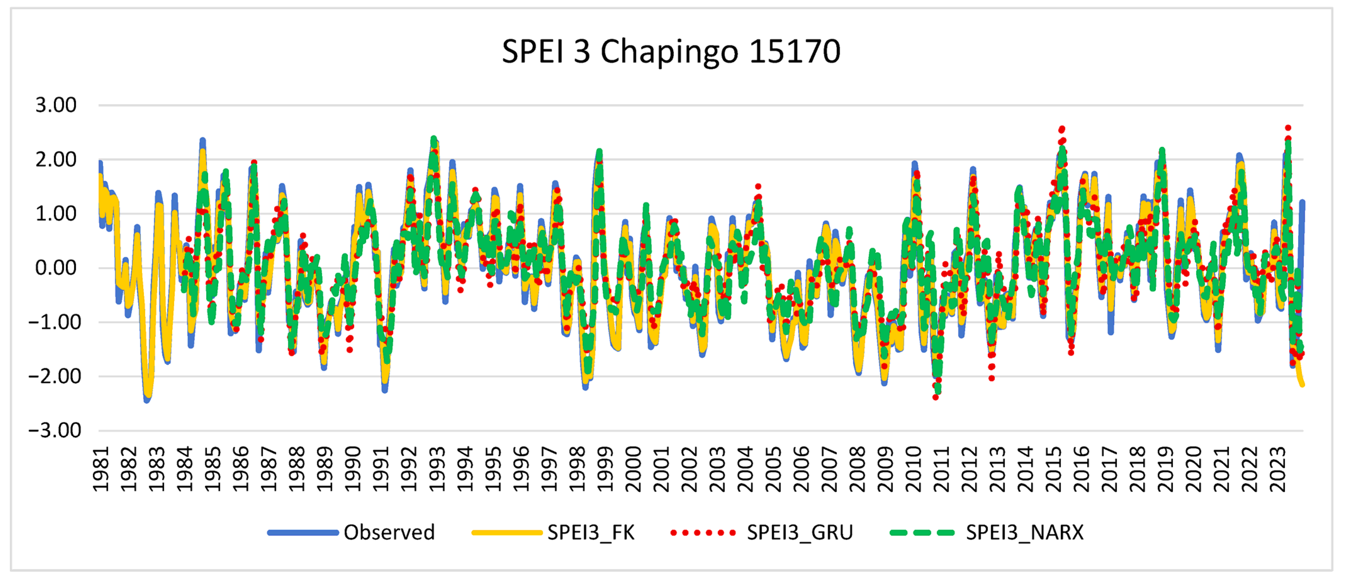
Figure 4 shows the temporal evolution of the observed SPEI3 index and the predictions generated by the FK, GRU, and NARX models, as well as their respective uncertainty bands (FK and GRU). It is observed that the FK model follows more accurately the interannual variability of SPEI 3 and maintains a narrower prediction band, indicating greater stability. In contrast, GRU presents greater dispersion in extreme events and NARX tends to smooth severe droughts, which could affect its early detection capability.

FK (Kalman filter) clearly outperforms GRU and NARX on all metrics. Both GRU and NARX present difficulties in capturing the SPEI3 structure, reflected in their low NSE and negative KGE. For practical applications, especially early warning systems or water planning, the FK model is the most reliable at this scale and time scale.

The FK was the best performing model in predicting the 3-month SPEI24 (Figure 5). The metrics reflect excellent fit, with low MAE (0.0325) and low RMSE (0.049), indicating accuracy and stability. R² and NSE ≈ 0.9975, showing an over-salient ability to replicate temporal variability. KGE ≈ 0.95, meaning that the model not only predicts accurately, but also preserves the statistical properties of the observed index. This is ideal for the prediction of prolonged droughts such as those captured by SPEI24. It also ensures high reliability for warning and water management systems.

The GRU model, despite having a good overall fit (R² and NSE ≈ 0.92), presents important limitations, with errors notoriously larger than FK (with an MAE of 0.10) and a negative KGE (−1.13), indicating that the model does not correctly replicate the structure of the index (bias, variability, and correlation). This suggests that although the GRU can follow the general trend, its statistical performance is inadequate. It is acceptable in trend, but not reliable for operational decisions without additional adjustments.

NARX slightly outperforms GRU in accuracy, with MAE ≈ 0.091 and RMSE ≈ 0.117, slightly better than GRU. R² and NSE ≈ 0.935, which are slightly higher too. However, KGE is still negative (−0.71), which compromises its use in statistical structure-sensitive applications. It is better than GRU, but still not competitive against FK. It has potential for improvement if hyperparameters are adjusted.

The Kalman filter (KF) is clearly superior for SPEI24 forecasting 3 months in advance (

Table 7. Average metrics of the 23 stations analyzed for a 3-month prediction with SPEI24.

Model	MAE	RMSE	R2	NSE	KGE	Global Evaluation
FK	0.0325	0.0490	0.9975	0.9975	0.95	Excellent
GRU	0.1003	0.1286	0.9207	0.9207	−1.13	Acceptable, but statistically weak
NARX	0.0913	0.1170	0.9348	0.9348	−0.71	Moderate, better than GRU but still deficient in structure

). Its ability to maintain accuracy, a low error spread, and statistical replication makes it the most reliable model. The GRU and NARX models, although offering acceptable R² and NSE values, fail to correctly reproduce the index structure (evidenced by their negative KGE values), which limits their practical applicability without significant adjustments.

4. Discussion

The results obtained in the present study show significant differences in the performance of the three models evaluated for the forecast of the Standardized Precipitation Evapotranspiration Index (SPEI), especially on medium- and long-term scales (

Table 8. Performance comparison by model for 3-month forecasting (averages over 23 stations).

SPEI	Model	MAE	RMSE	R2	NSE	KGE	Global Evaluation
SPEI1	FK	0.403	0.513	0.728	0.728	−6.02	Weak
SPEI1	GRU	0.244	0.307	0.204	0.204	−0.13	Very low
SPEI1	NARX	0.242	0.302	0.226	0.226	−0.08	Very low
SPEI3	FK	0.101	0.132	0.982	0.982	0.85	Excellent
SPEI3	GRU	0.167	0.213	0.697	0.697	−3.34	Unstable
SPEI3	NARX	0.170	0.217	0.691	0.691	−0.51	Could be improved
SPEI6	FK	0.073	0.096	0.990	0.990	0.91	Very good
SPEI6	GRU	0.152	0.193	0.776	0.776	−2.73	Low
SPEI6	NARX	0.147	0.185	0.796	0.796	−0.72	Moderate
SPEI9	FK	0.053	0.073	0.994	0.994	0.95	Very good
SPEI9	GRU	0.128	0.166	0.844	0.844	−1.39	Acceptable
SPEI9	NARX	0.124	0.160	0.856	0.856	−0.15	Could be improved
SPEI12	FK	0.041	0.061	0.996	0.996	0.96	Excellent
SPEI12	GRU	0.096	0.126	0.909	0.909	−0.88	Acceptable
SPEI12	NARX	0.099	0.129	0.905	0.905	0.08	Moderate
SPEI24	FK	0.033	0.049	0.997	0.997	0.95	Excellent
SPEI24	GRU	0.100	0.129	0.921	0.921	−1.13	Acceptable
SPEI24	NARX	0.091	0.117	0.935	0.935	−0.71	Moderate

). Although all models showed high levels of accuracy in terms of R² and NSE (above 0.97), a more detailed analysis of complementary metrics such as MAE, RMSE, and especially Kling–Gupta efficiency (KGE) allows clearer advantages and limitations to be established between the approaches.

FK (Kalman filter) is the best model at all SPEI scales (Table 8), except at SPEI1 where all models fail. GRU performs acceptably at SPEI9–SPEI24 but has significant instability at short scales such as SPEI1–SPEI3. NARX is competitive at SPEI9–SPEI24, although its negative KGE on many scales suggests that it does not replicate well the statistical structure of the observed SPEI.

The NARX model (autoregressive neural networks with external input) proved to be the most accurate, with the lowest mean absolute error (MAE = 0.098) and the highest KGE (0.864). This indicates that NARX not only achieves high correlation with the observed data, but also adequately reproduces the natural variability of SPEI, without notable systematic biases. Its ability to incorporate extemporaneous inputs and maintain long-term memory makes it particularly suitable for predicting cumulative climate indicators such as SPEI, especially at scales such as SPEI6 to SPEI12.

On the other hand, the GRU (gated recurrent unit) model showed a performance very close to that of NARX, with an MAE of 0.101 and a KGE of 0.829. GRU, being a simplified recurrent architecture with respect to LSTM, offers an additional advantage in terms of computational efficiency and lower training complexity. Its good performance, especially at the SPEI3 and SPEI6 scales, makes it a viable option for applications where fast response is required or limited computational resources are available.

In comparison, the FK model (Kalman filter with exogenous variables, DKF-ARX-Pt), although achieving an R² of 0.976 and an NSE of the same value, showed lower performance on the KGE metric (0.735). This suggests that, although the model can accurately capture the overall trend of the index, it has more difficulty in faithfully representing the dispersion and error structure, especially at short scales such as SPEI1, where its performance was significantly lower (KGE < 0). Nevertheless, the FK model is still useful for long scales (SPEI12 and SPEI24), where its dynamic structure makes it stable and less susceptible to overfitting.

A key aspect in the discussion is the role of the SPEI scale in the performance of the models. It was confirmed that the intermediate scales (SPEI3 to SPEI12) represent the best compromise between sensitivity and predictive stability. The SPEI1 scale, due to its high variability and dependence on very short-term weather events, presented high errors and lower reliability for all models, while SPEI24, although stable, smooths the data too much and may miss critical information on rapid drought events.

As shown in Table 5, the NARX model achieves the lowest average error metrics (MAE and RMSE) and the highest values in R², NSE, and KGE, indicating excellent predictive accuracy on average. However, despite its strong performance, NARX presents challenges in computational demand and occasional instability in training convergence, especially when applied to data-sparse stations or longer SPEI time scales. FK also consistently produced positive KGE and NSE values across nearly all stations, while NARX exhibited performance degradation and instability at short time scales. This justifies our conclusion that FK is the most reliable model overall, especially for long-term drought forecasting and risk analysis.

In addition, the analysis revealed that models with memory (GRU and NARX) tend to perform better than FK, especially in prediction horizons of 3 to 6 months, which is highly relevant for early warning systems, where changes in water conditions need to be anticipated in time to plan mitigation measures.

5. Conclusions

The present comparative analysis of Standardized Precipitation Evapotranspiration Index (SPEI) prediction models at multiple time scales (SPEI1 to SPEI24) and for 3- and 6-month horizons demonstrates key differences in model performance. While the NARX model achieved the best average metrics (the lowest MAE and RMSE, and the highest R², NSE, and KGE), it exhibited instability and higher computational costs, limiting its applicability in real-time or data-scarce contexts.

In contrast, the DKF-ARX-Pt (Kalman filter) model proved to be the most consistent and robust across stations and SPEI scales. It achieved high accuracy (R² and NSE > 0.97), low error dispersion, and positive KGE values at almost all scales—especially at medium and long scales such as SPEI6, SPEI12, and SPEI24. Its low computational demand and stable behavior make it highly suitable for early warning systems, drought risk monitoring, and climate adaptation strategies.

GRU showed competitive performance at intermediate scales, with relatively low training complexity, but its performance varied more across stations and lead times. All models struggled to predict SPEI1 reliably, reflecting the challenges of capturing short-term variability in climate systems.

In summary, FK offers the best trade-off between accuracy, generalization, and computational efficiency. While NARX and GRU demonstrate potential, their practical deployment would require further tuning and computational resources. This study supports the FK model as a strong candidate for operational drought forecasting in Central Mexico, especially under resource-limited or real-time conditions.