

Effects of Variations in Water Table Orientation on LNAPL Migration Processes

Abstract
1. Introduction
2. Mathematical Model of LNAPL Migration Under Variations in Water Table Orientation
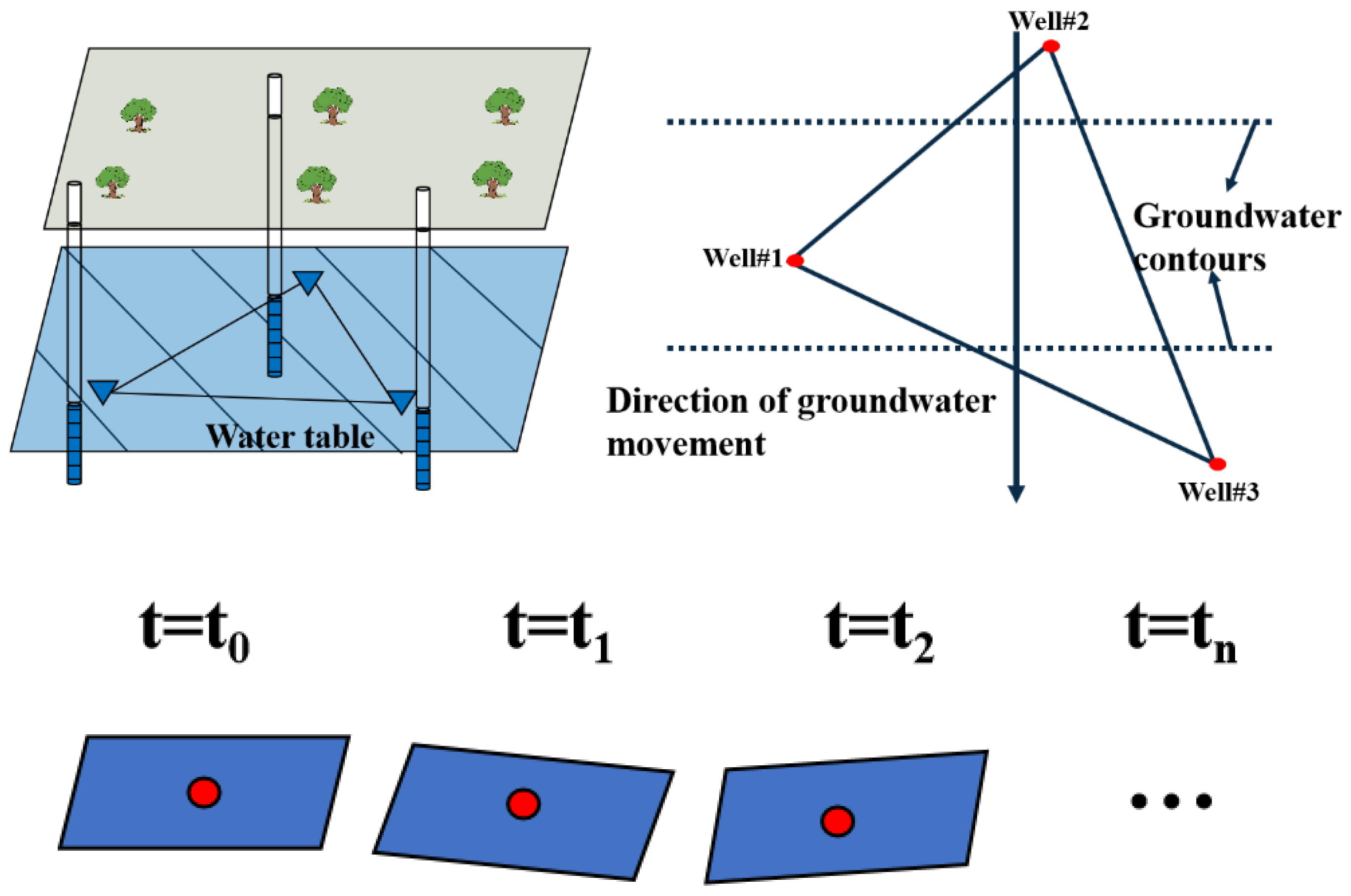
2.1. Equation for Variations in Water Table Orientation
2.2. Conservation of Momentum Equation
2.3. Constitutive Model
2.4. Temperature Variation Equation
3. Case Study and Model Construction
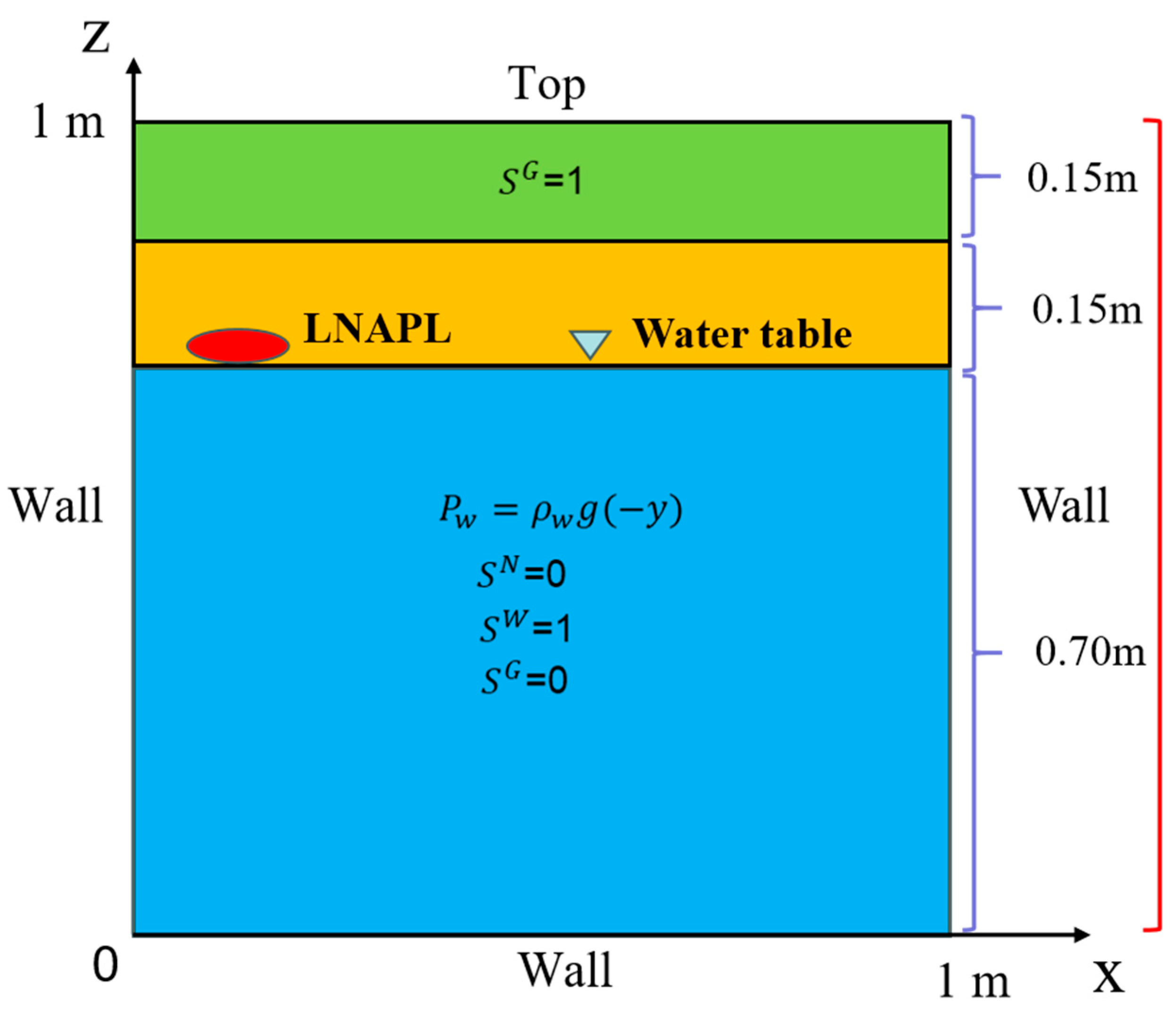
Overview of Case Study and Initial and Boundary Conditions
- (1)
- Flow field
- (2)
- Chemical field
4. Results
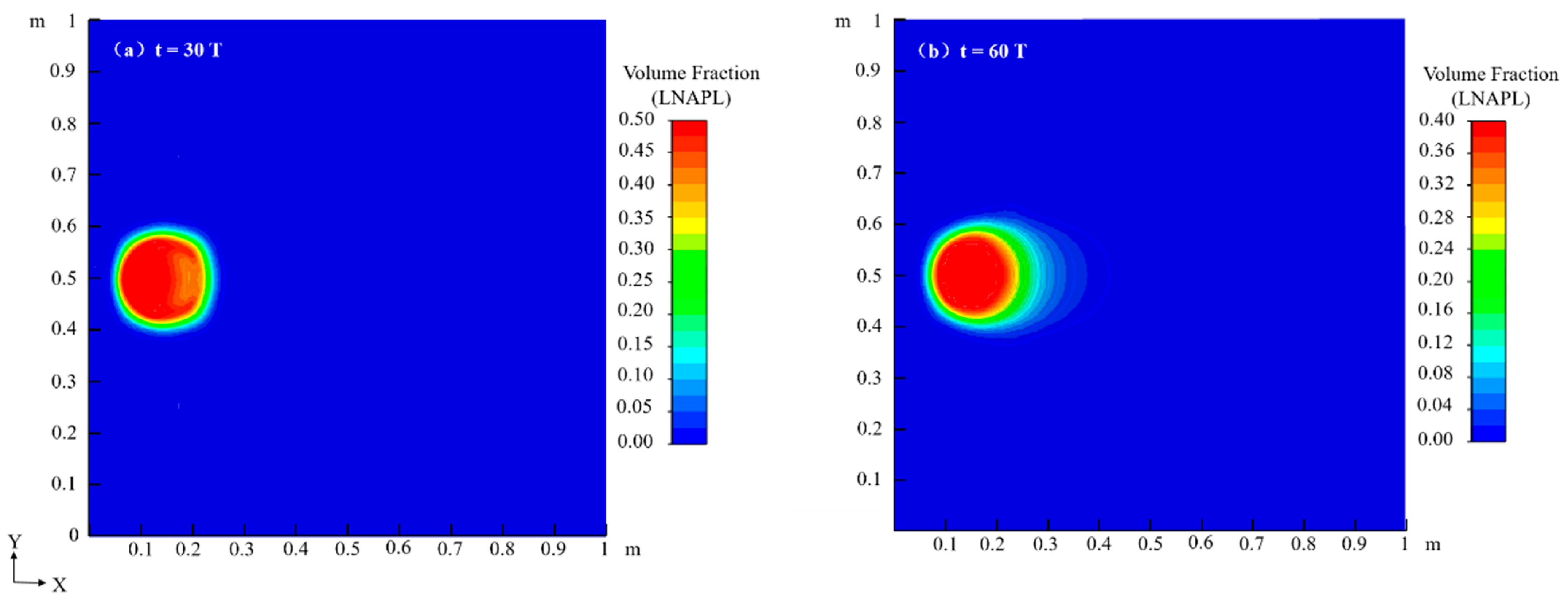
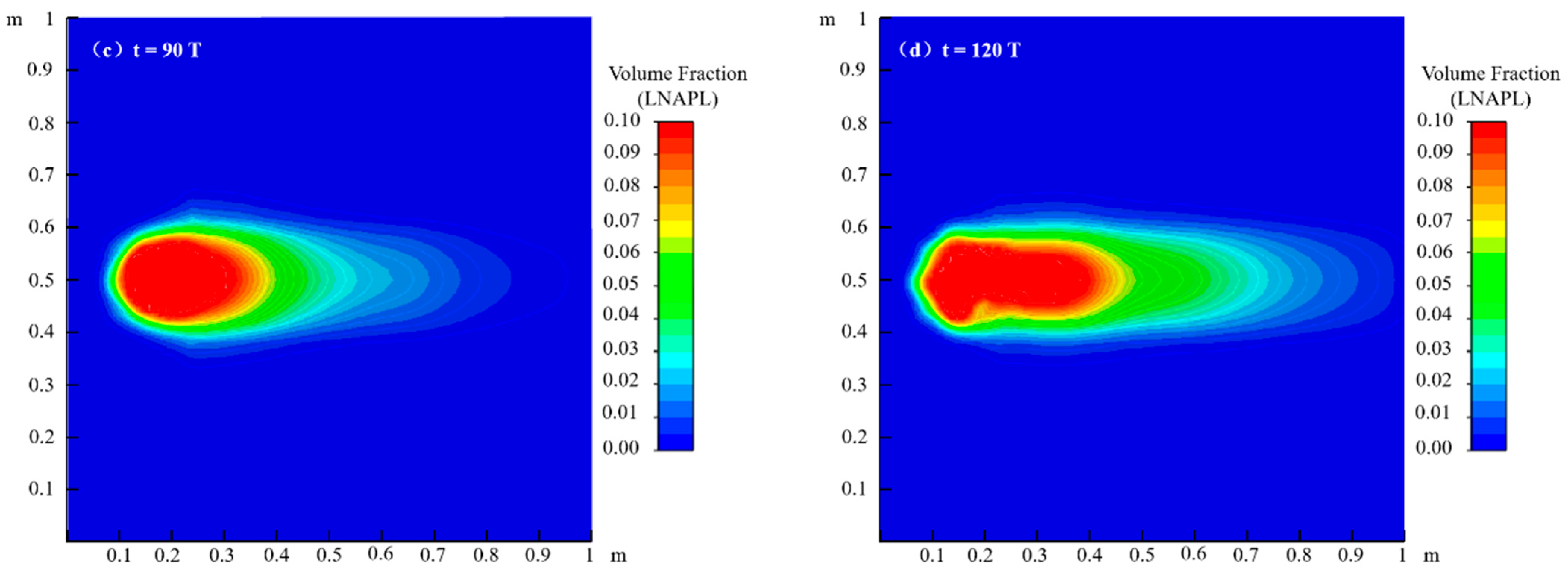
4.1. Migration Process of LNAPL Without Variations in Water Table Orientation
4.1.1. Flow Field
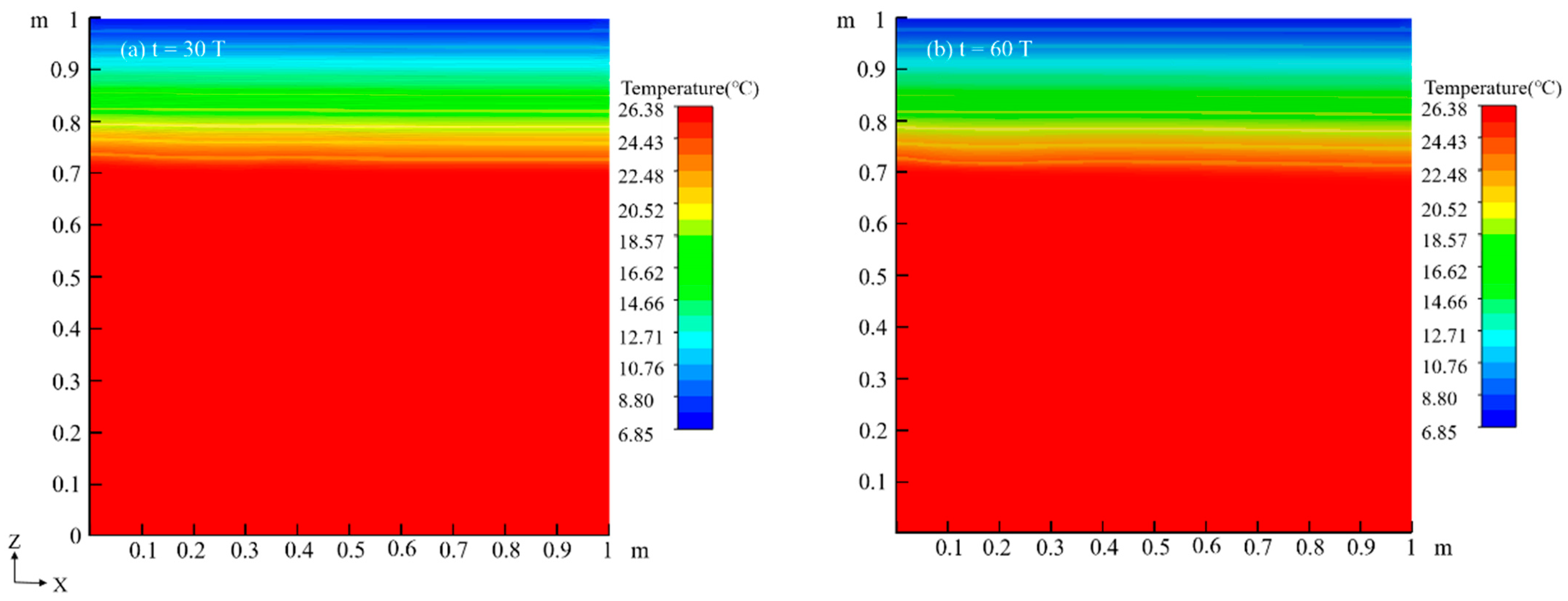
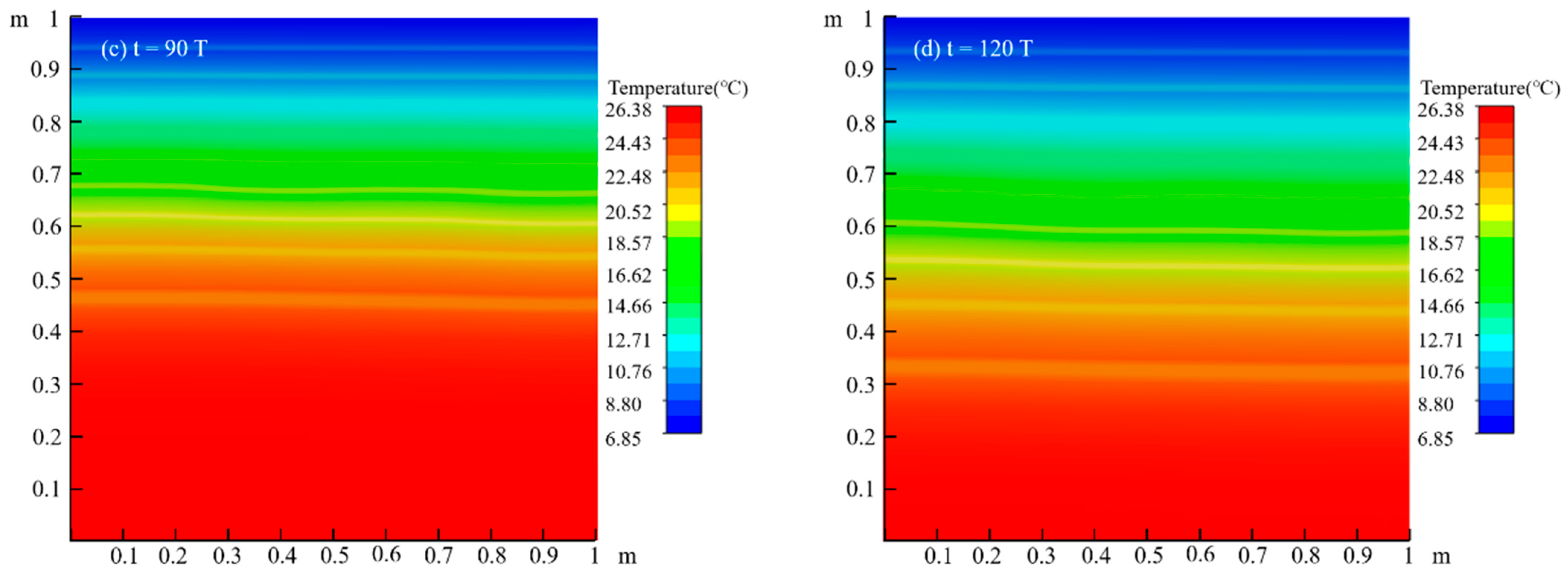
4.1.2. Temperature Field
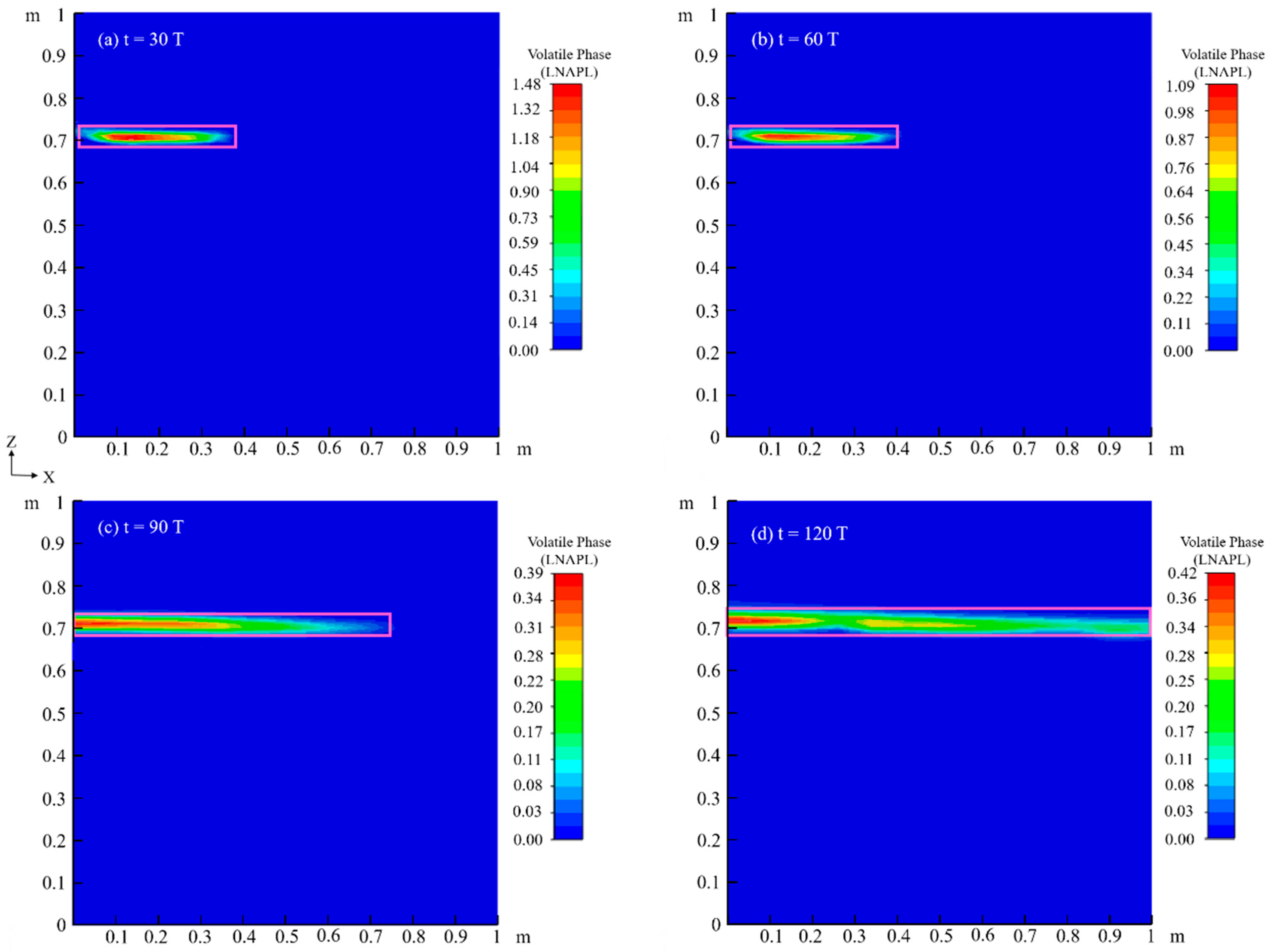
4.2. Migration Process of LNAPL with Variations in Water Table Orientation
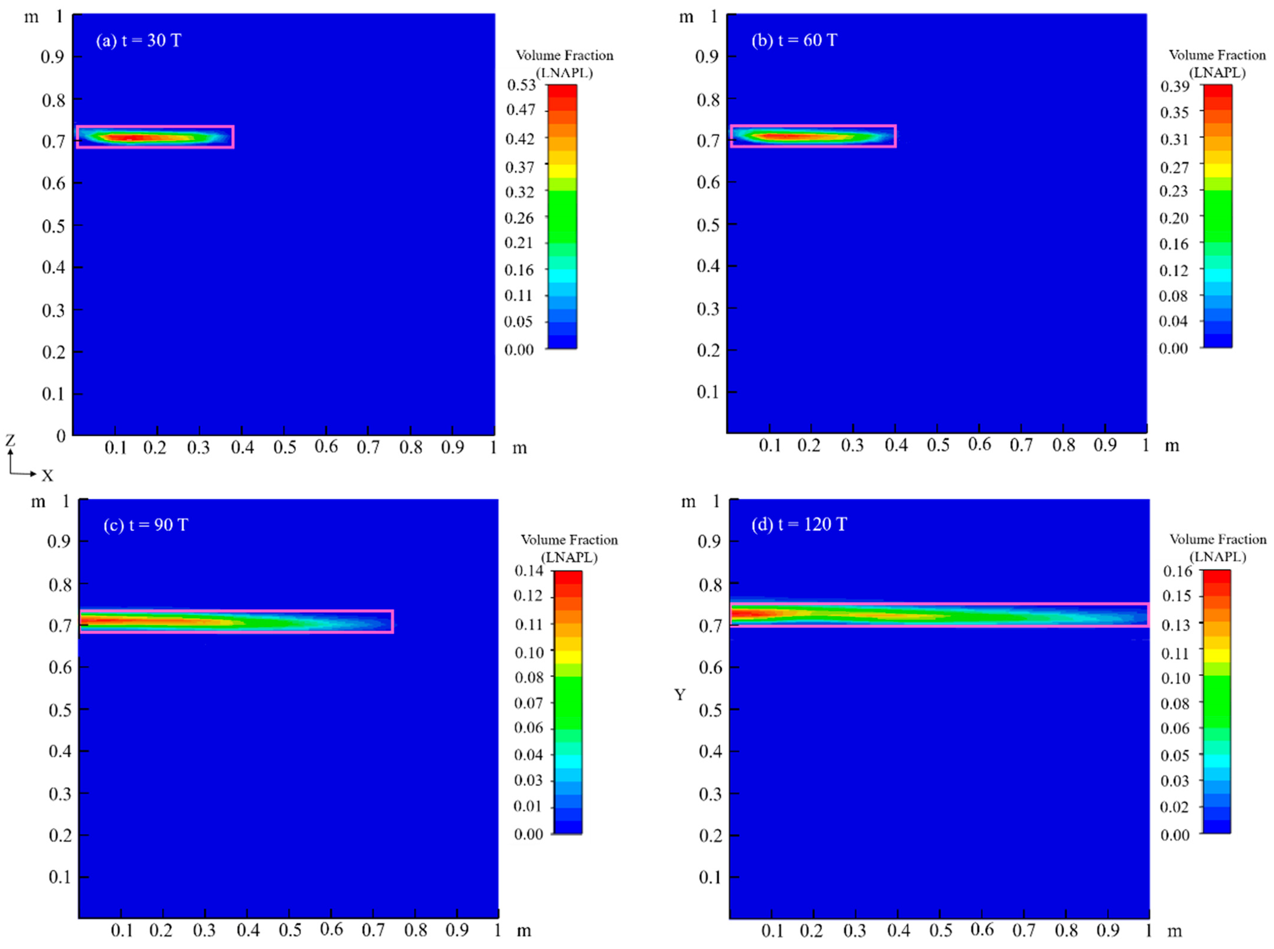
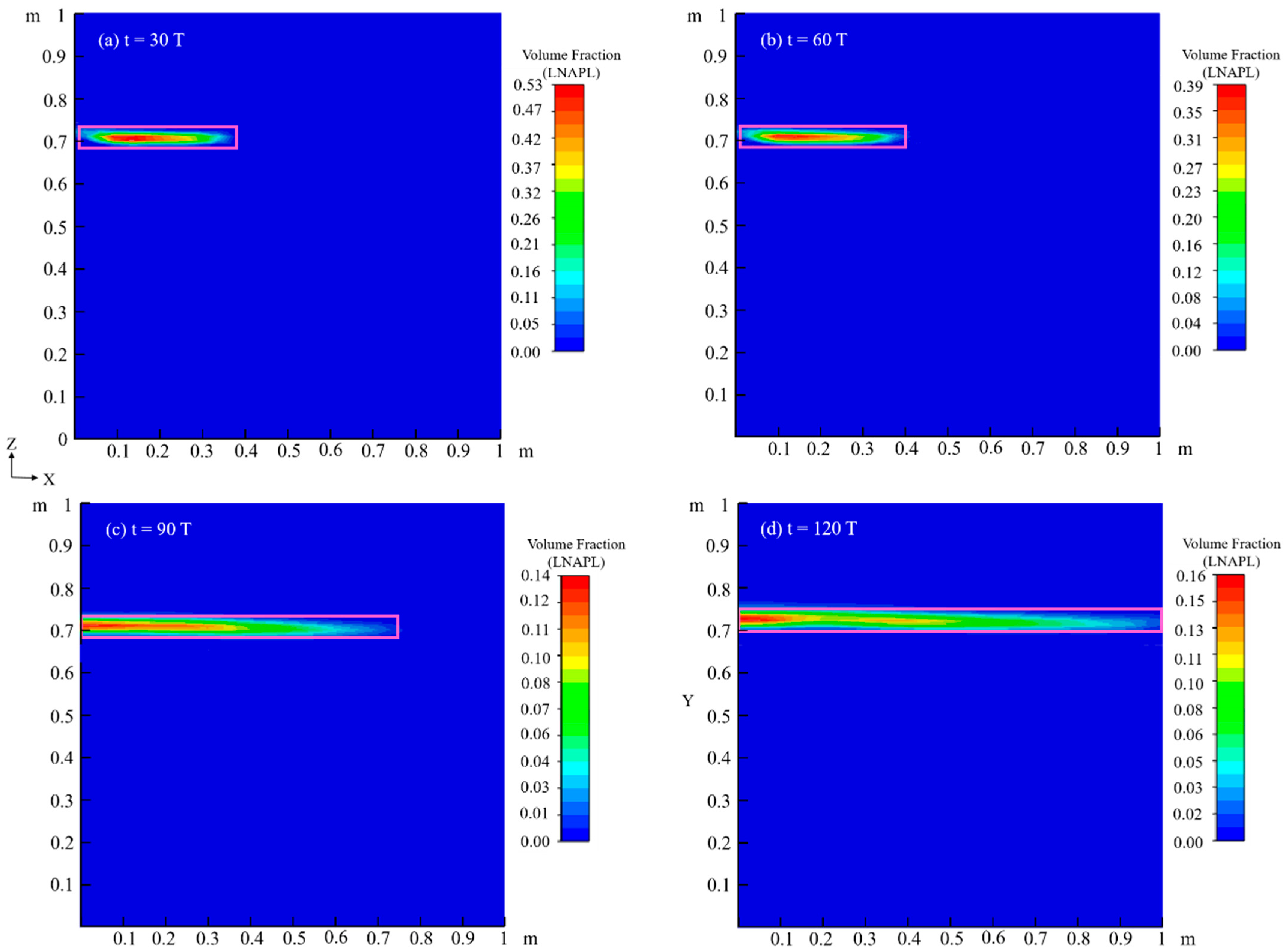
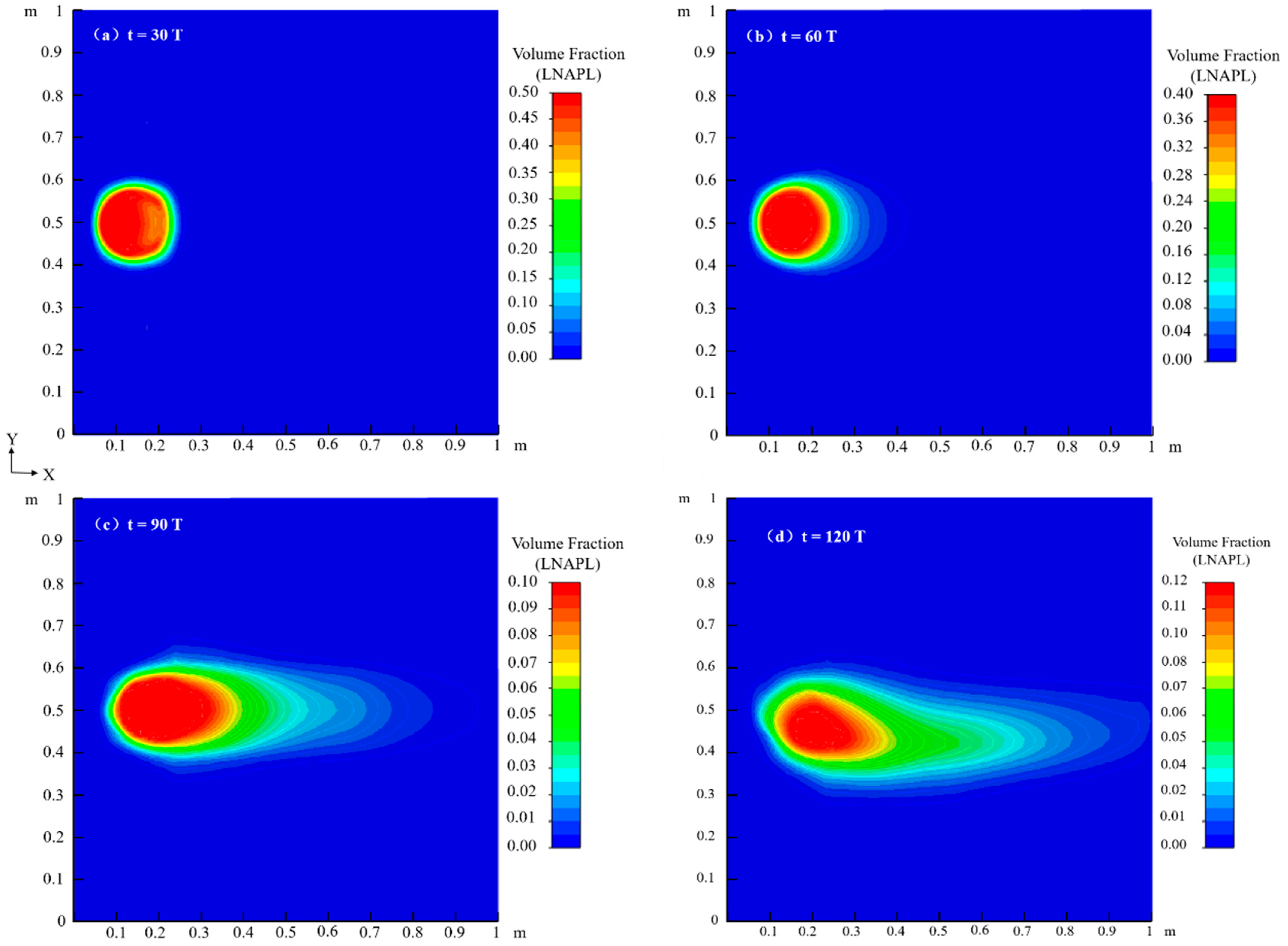
4.2.1. Flow Field
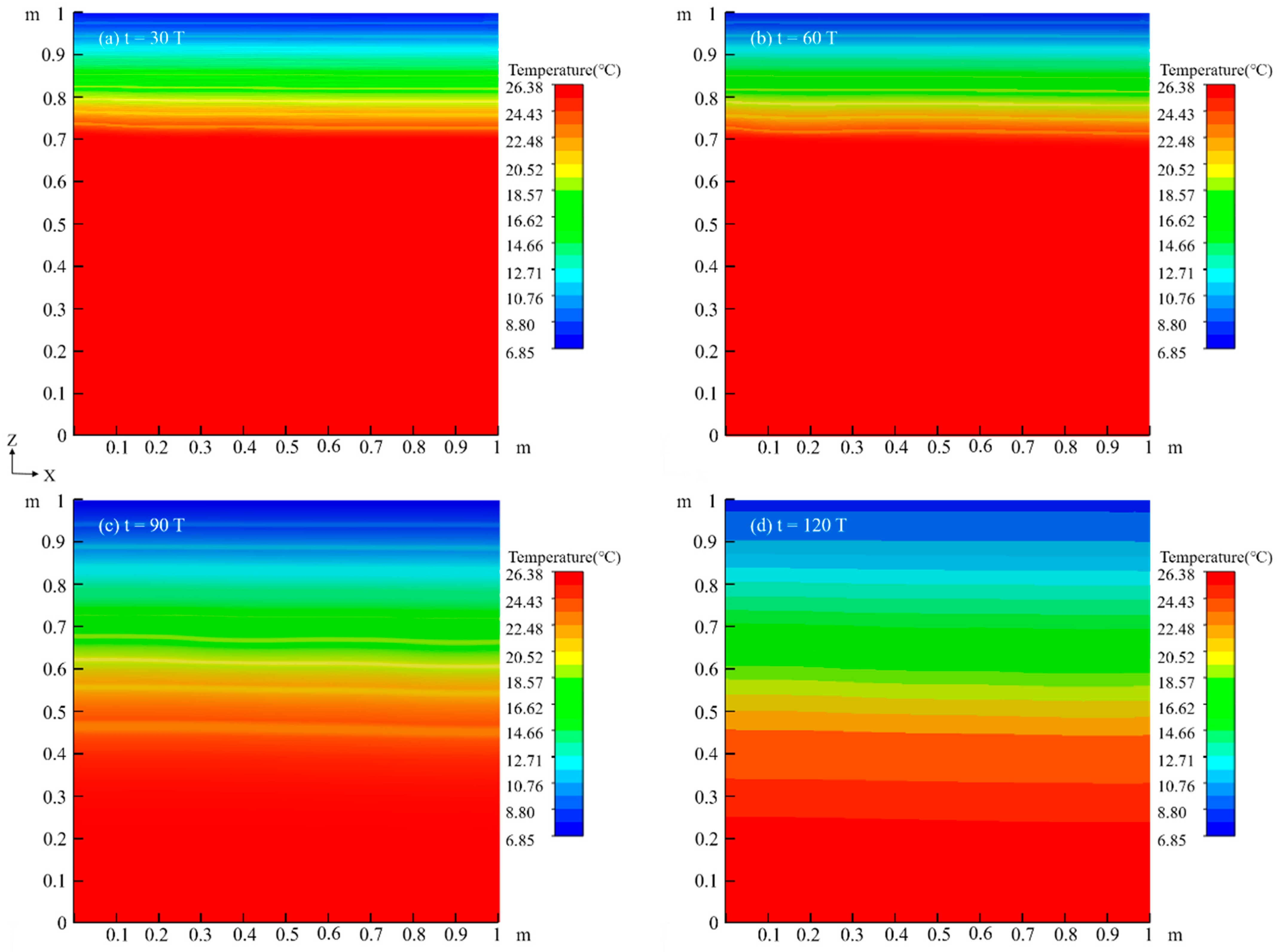
4.2.2. Temperature Field
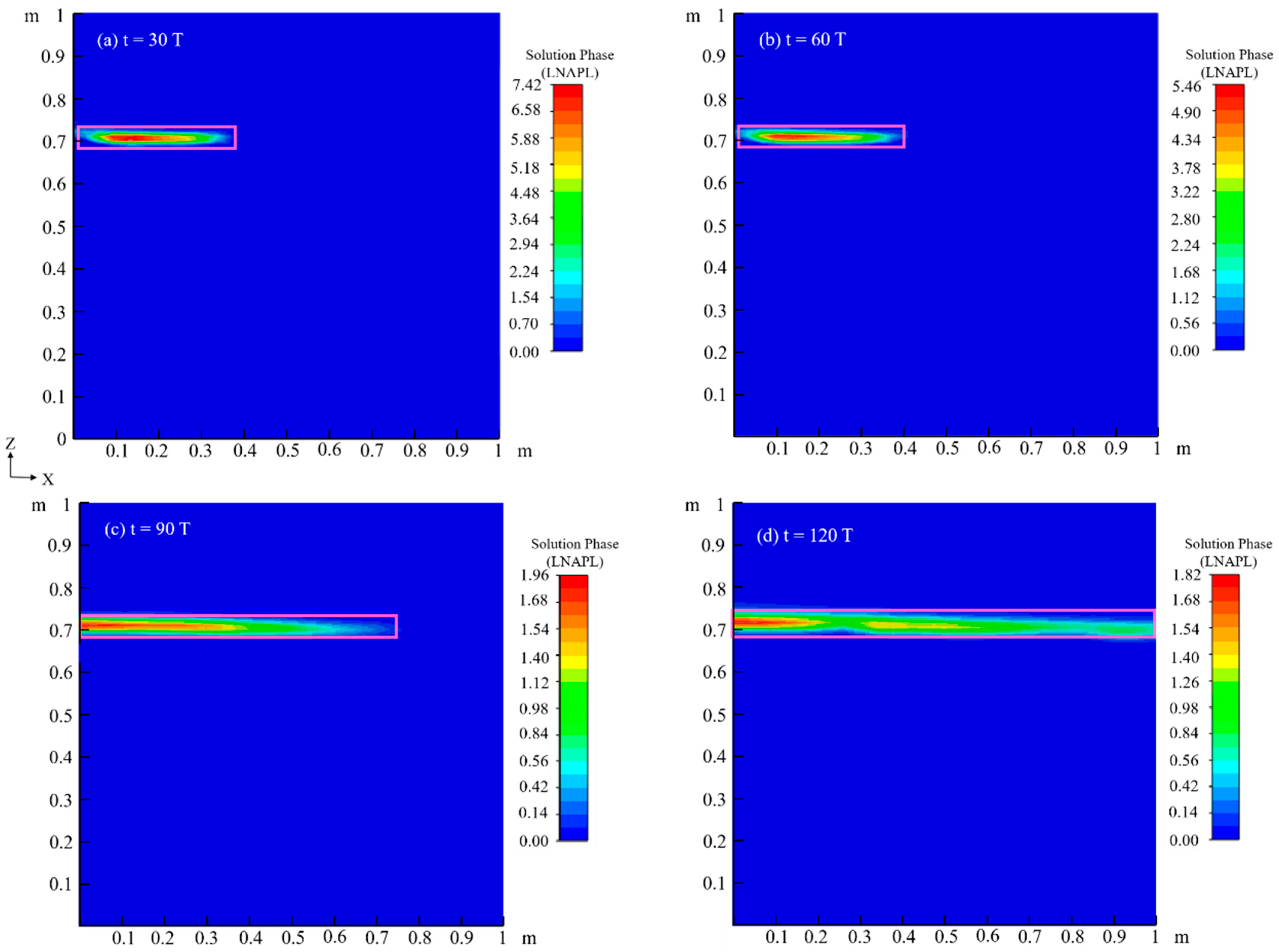
4.2.3. Chemical Field
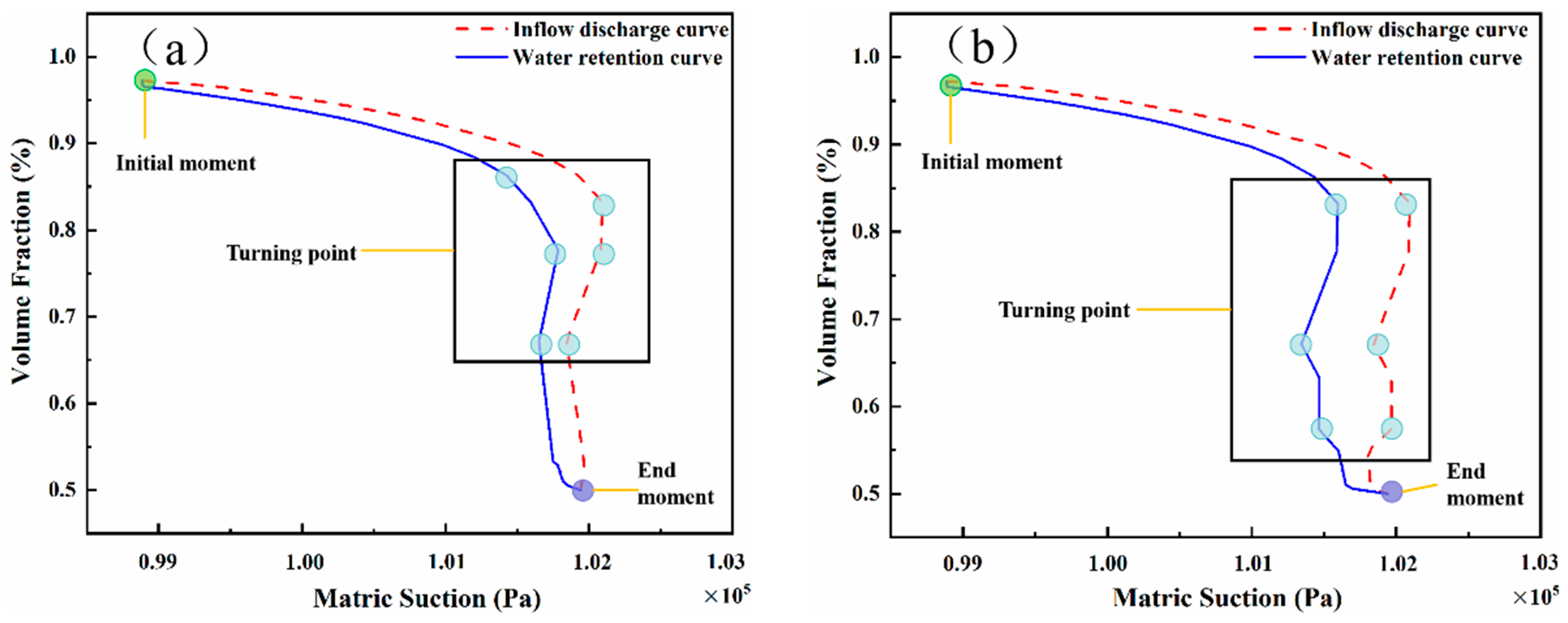
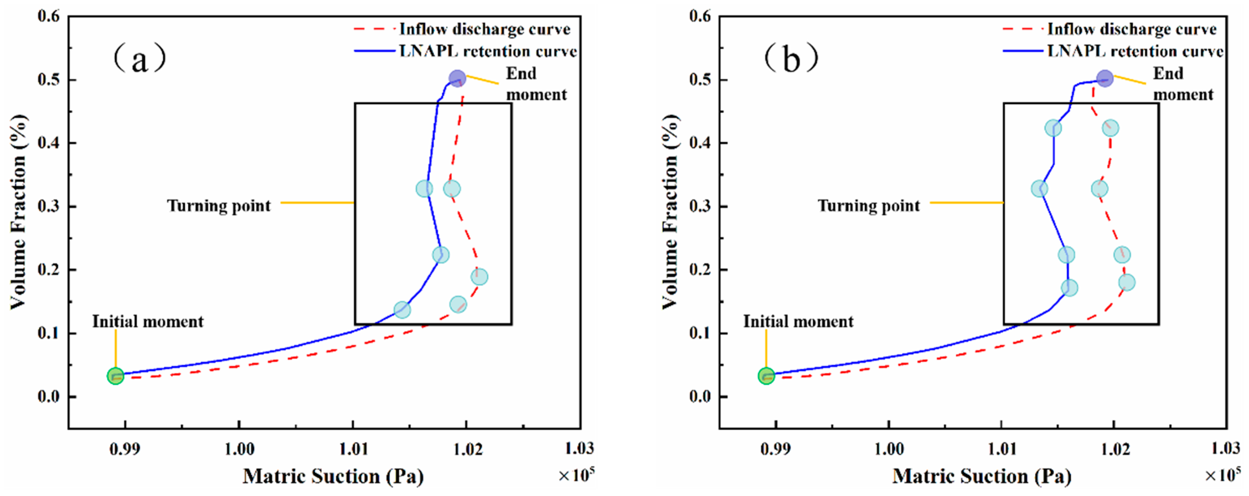
4.3. Effects of Capillary Action on LNAPL Migration Distribution with Variations in Water Table Orientation
5. Discussion
6. Conclusions
Author Contributions
Funding
Data Availability Statement
Acknowledgments
Conflicts of Interest
References
- Maire, J.; Joubert, A.; Kaifas, D.; Invernizzi, T.; Marduel, J.; Colombano, S.; Cazaux, D.; Marion, C.; Klein, P.-Y.; Dumestre, A.; et al. Assessment of flushing methods for the removal of heavy chlorinated compounds DNAPL in an alluvial aquifer. Sci. Total Environ. 2018, 612, 1149–1158. [Google Scholar] [CrossRef] [PubMed]
- Alazaiza, M.Y.; Copty, N.K.; Abunada, Z. Experimental investigation of cosolvent flushing of DNAPL in double-porosity soil using light transmission visualization. J. Hydrol. 2020, 584, 124659. [Google Scholar] [CrossRef]
- Qiang, S.; Shi, X.; Revil, A.; Kang, X.; Liu, Y.; Wu, J. Residual NAPL morphology effects on electrical resistivity: Insights from micromodel displacement experiments and pore network simulations. Water Resour. Res. 2022, 58, e2022WR033233. [Google Scholar] [CrossRef]
- Xu, J.-C.; Yang, L.-H.; Yuan, J.-X.; Li, S.-Q.; Peng, K.-M.; Lu, L.-J.; Huang, X.-F.; Liu, J. Coupling surfactants with ISCO for remediation of NAPLs: Recent progress and application challenges. Chemosphere 2022, 303, 135004. [Google Scholar] [CrossRef]
- Mateas, D.; Tick, G.; Carroll, K. In situ stabilization of NAPL contaminant source-zones as a remediation technique to reduce mass discharge and flux to groundwater. J. Contam. Hydrol. 2017, 204, 40–56. [Google Scholar] [CrossRef]
- Shi, Y.; Sun, Y.; Gao, B.; Xu, H.; Shi, X.; Wu, J. Retention and Transport of Bisphenol A and Bisphenol S in Saturated Limestone Porous Media. Water Air Soil. Pollut. 2018, 229, 260. [Google Scholar] [CrossRef]
- Kechavarzi, C.; Soga, K.; Illangasekare, T.; Nikolopoulos, P. Laboratory Study of Immiscible Contaminant Flow in Unsaturated Layered Sandy soils. Vadose Zone J. 2008, 7, 1–9. [Google Scholar] [CrossRef]
- Simantiraki, F.; Aivalioti, M.; Gidarakos, E. Implementation of an image analysis technique to determine LNAPL infiltration and distribution in unsaturated porous media. Desalination 2009, 248, 705–715. [Google Scholar] [CrossRef]
- Pan, Y.; Yang, J.; Jia, Y.; Xu, Z. Experimental study on non-aqueous phase liquid multiphase flow characteristics and controlling factors in heterogeneous porous media. Environ. Earth Sci. 2016, 75, 75. [Google Scholar] [CrossRef]
- Teng, Y. Analysis of the LNAPL Migration Process in the Vadose Zone under Two Different Media Conditions. Int. J. Environ. Res. Public. Health 2021, 18, 11073. [Google Scholar] [CrossRef]
- Man, J.; Zhou, Q.; Wang, G.; Yao, Y. Modeling and evaluation of NAPL-impacted soil vapor intrusion facilitated by vadose zone breathing. J. Hydrol. 2022, 615, 128683. [Google Scholar] [CrossRef]
- Suk, H.; Zheng, K.; Liao, Z.; Liang, C.; Wang, S.; Chen, J. A new analytical model for transport of multiple contaminants considering remediation of both NAPL source and downgradient contaminant plume in groundwater. Adv. Water Resour. 2022, 167, 104290. [Google Scholar] [CrossRef]
- Cavelan, A.; Golfier, F.; Colombano, S.; Davarzani, H.; Deparis, J.; Faure, P. A critical review of the influence of groundwater level fluctuations and temperature on LNAPL contaminations in the context of climate variations. Sci. Total. Environ. 2022, 806, 150412. [Google Scholar] [CrossRef] [PubMed]
- Gatsios, E.; Jonás, G.; Rayner, J.L.; McLaughlan, R.G.; Davis, G.B. LNAPL transmissivity as a remediation metric in complex sites under water table fluctuations. J. Environ. Manag. 2018, 215, 40–48. [Google Scholar] [CrossRef] [PubMed]
- Onaa, C.; Olaobaju, E.A.; Amro, M.M. Experimental and numerical assessment of light non-aqueous phase liquid (LNAPL) subsurface migration behavior in the vicinity of groundwater table. Environ. Technol. Innov. 2021, 23, 101573. [Google Scholar] [CrossRef]
- Libera, A.; Barros, F.P.J.; Guadagnini, A. Influence of pumping operational schedule on solute concentrations at a well in randomly heterogeneous aquifers. J. Hydrol. 2017, 546, 490–502. [Google Scholar] [CrossRef]
- Atlabachew, A.; Shu, L.; Wu, P.; Zhang, Y.; Xu, Y. Numerical modeling of solute transport in a sandy soil tank physical model under varying hydraulic gradient and hydrological stresses. Hydrogeol. J. 2018, 26, 2089–2113. [Google Scholar] [CrossRef]
- Bai, Q.; Li, X.; Tian, Y.; Fang, J. Equations and numerical simulation for coupled water and heat transfer in frozen soil. Chin. J. Geotech. Eng. 2015, 37, 131–136. [Google Scholar] [CrossRef]
- Gao, Y. Particle tracking using dynamic water-level data. Water 2020, 12, 2063. [Google Scholar] [CrossRef]
- Kacem, M.; Benadda, B. Mathematical Model for Multiphase Extraction Simulation. J. Environ. Eng. 2018, 144, 04018040. [Google Scholar] [CrossRef]
- Parker, J.C.; Lenhard, R.J.; Kuppusamy, T. A parametric model for constitutive properties governing multiphase flow in porous media. Water Resour. Res. 1987, 23, 618–624. [Google Scholar] [CrossRef]
- Dou, Z.; Chen, Y.C.; Zhuang, C.; Zhou, Z.F.; Wang, J.G. Emergence of non-aqueous phase liquids redistribution driven by freeze-thaw cycles in porous media based on low-field NMR. J. Hydrol. 2022, 612, 128106. [Google Scholar] [CrossRef]
- Kacem, M.; Esrael, D.; Boeije, C.S.; Benadda, B. Multiphase Flow Model for NAPL Infiltration in Both the Unsaturated and Saturated Zones. J. Environ. Eng. 2019, 145, 04019072. [Google Scholar] [CrossRef]
- Millington, R.J. Gas Diffusion in Porous Media. Science 1959, 130, 100–102. [Google Scholar] [CrossRef]
- Zhang, M.L.; Wen, Z.; Xue, K.; Chen, L.Z.; Li, D.S. A coupled model for liquid water, water vapor and heat transport of saturated-unsaturated soil in cold regions: Model formulation and calibration. Environ. Earth Sci. 2016, 75, 701. [Google Scholar] [CrossRef]
- Luo, C.-L.; Yu, Y.-Y.; Zhang, J.; Tao, J.-Y.; Ou, Q.-J.; Cui, W.-H. Thermal-water-salt coupling process of unsaturated saline soil under unidirectional freezing. J. Mt. Sci. 2023, 20, 557–569. [Google Scholar] [CrossRef]
- Parker, J.C.; Lenhard, R.J. Determining three-phase permeability—Saturation—Pressure relations from two-phase system measurements. J. Pet. Sci. Eng. 1990, 4, 57–65. [Google Scholar] [CrossRef]
- Wang, C.; Su, X.; Lyu, H.; Yuan, Z. Remobilization of LNAPL in unsaturated porous media subject to freeze-thaw cycles using modified light transmission visualization technique. J. Hydrol. 2021, 603, 127090. [Google Scholar] [CrossRef]
- Zhang, J.; Lai, Y.; Li, J.; Zhao, Y. Study on the influence of hydro-thermal-salt-mechanical interaction in saturated frozen sulfate saline soil based on crystallization kinetics. Int. J. Heat. Mass. Transf. 2020, 146, 118868. [Google Scholar] [CrossRef]
- Koohbor, B.; Colombano, S.; Harrouet, T.; Deparis, J.; Lion, F.; Davarzani, D.; Ataie-Ashtiani, B. The effects of water table fluctuation on LNAPL deposit in highly permeable porous media: A coupled numerical and experimental study. J. Contam. Hydrol. 2023, 256, 104183. [Google Scholar] [CrossRef]
- Ismail, R.; Al-Raoush, R.; Alazaiza, M. The impact of water table fluctuation and salinity on LNAPL distribution and geochemical properties in the smear zone under completely anaerobic conditions. Environ. Earth Sci. 2023, 82, 368. [Google Scholar] [CrossRef]
- Huntley, D.; Beckett, G. Persistence of LNAPL sources: Relationship between risk reduction and LNAPL recovery. J. Contam. Hydrol. 2002, 59, 3–26. [Google Scholar] [CrossRef] [PubMed]

| Material | Quality | Parameter | Value |
|---|---|---|---|
| Soil | -VG Model parameters | 6.1 | |
| -VG Model parameters | 6 | ||
| -VG Model parameters | 0.83 | ||
| -VG Model parameters | 0.5 | ||
| porosity | 0.445 | ||
| Specific heat capacity of the soil | 722 | ||
| Organic carbon content | 0.03 | ||
| LNAPL Phase | LNAPL density | 700 | |
| LNAPL Phase viscosity | 0.0017 | ||
| LNAPL Specific heat capacity | 1006.43 | ||
| LNAPL Thermal conductivity | 0.0242 | ||
| LNAPL Henry’s constant | 0.27 | ||
| Water Phase | Water density | 998.2 | |
| Gravitational acceleration | −9.80999 | ||
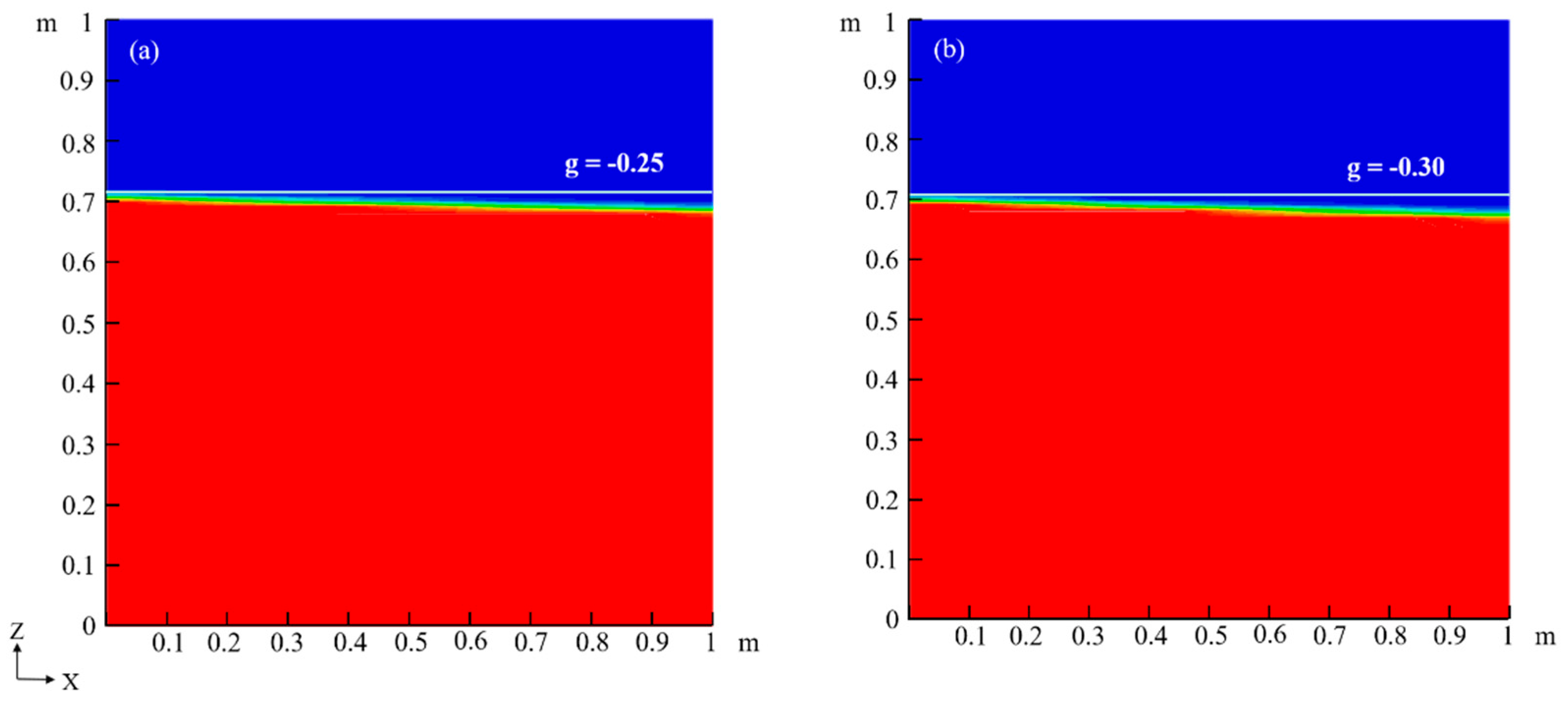
| −0.25 | |||
| −0.3 | |||
| Aqueous viscosity | 0.001003 | ||
| Water thermal conductivity | 0.55 | ||
| Water compared to heat capacity | 4182 |
Disclaimer/Publisher’s Note: The statements, opinions and data contained in all publications are solely those of the individual author(s) and contributor(s) and not of MDPI and/or the editor(s). MDPI and/or the editor(s) disclaim responsibility for any injury to people or property resulting from any ideas, methods, instructions or products referred to in the content. |
© 2025 by the authors. Licensee MDPI, Basel, Switzerland. This article is an open access article distributed under the terms and conditions of the Creative Commons Attribution (CC BY) license (https://creativecommons.org/licenses/by/4.0/).
Share and Cite
Yu, H.; Guan, Q.; Zhao, X.; He, H.; Chen, L.; Gao, Y. Effects of Variations in Water Table Orientation on LNAPL Migration Processes. Water 2025, 17, 1989. https://doi.org/10.3390/w17131989
Yu H, Guan Q, Zhao X, He H, Chen L, Gao Y. Effects of Variations in Water Table Orientation on LNAPL Migration Processes. Water. 2025; 17(13):1989. https://doi.org/10.3390/w17131989
Chicago/Turabian StyleYu, Huiming, Qingqing Guan, Xianju Zhao, Hongguang He, Li Chen, and Yuan Gao. 2025. "Effects of Variations in Water Table Orientation on LNAPL Migration Processes" Water 17, no. 13: 1989. https://doi.org/10.3390/w17131989
APA StyleYu, H., Guan, Q., Zhao, X., He, H., Chen, L., & Gao, Y. (2025). Effects of Variations in Water Table Orientation on LNAPL Migration Processes. Water, 17(13), 1989. https://doi.org/10.3390/w17131989