

Towards a Realistic Data-Driven Leak Localization in Water Distribution Networks


Abstract
1. Introduction
2. Methodology
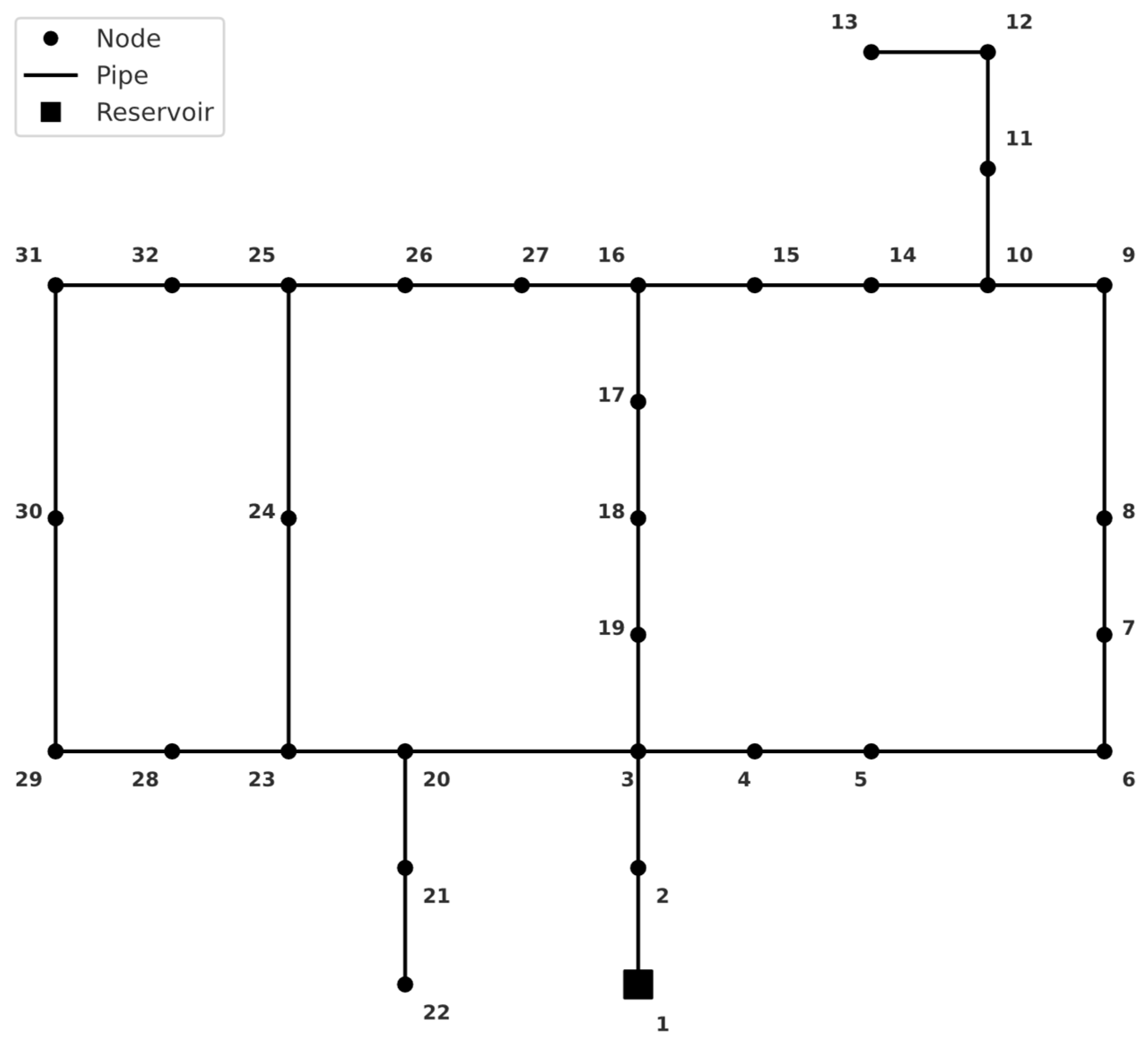
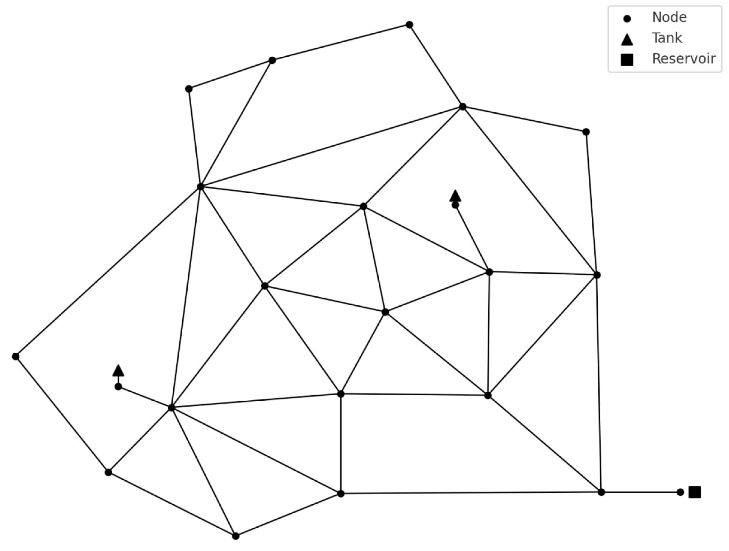
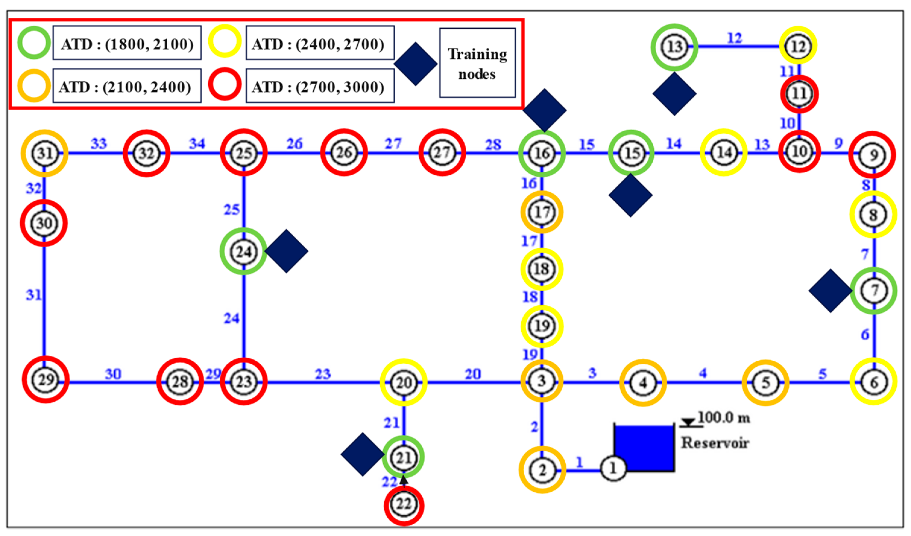
2.1. Benchmark Networks
- (a)
- Hanoi network
- (b)
- Anytown WDN
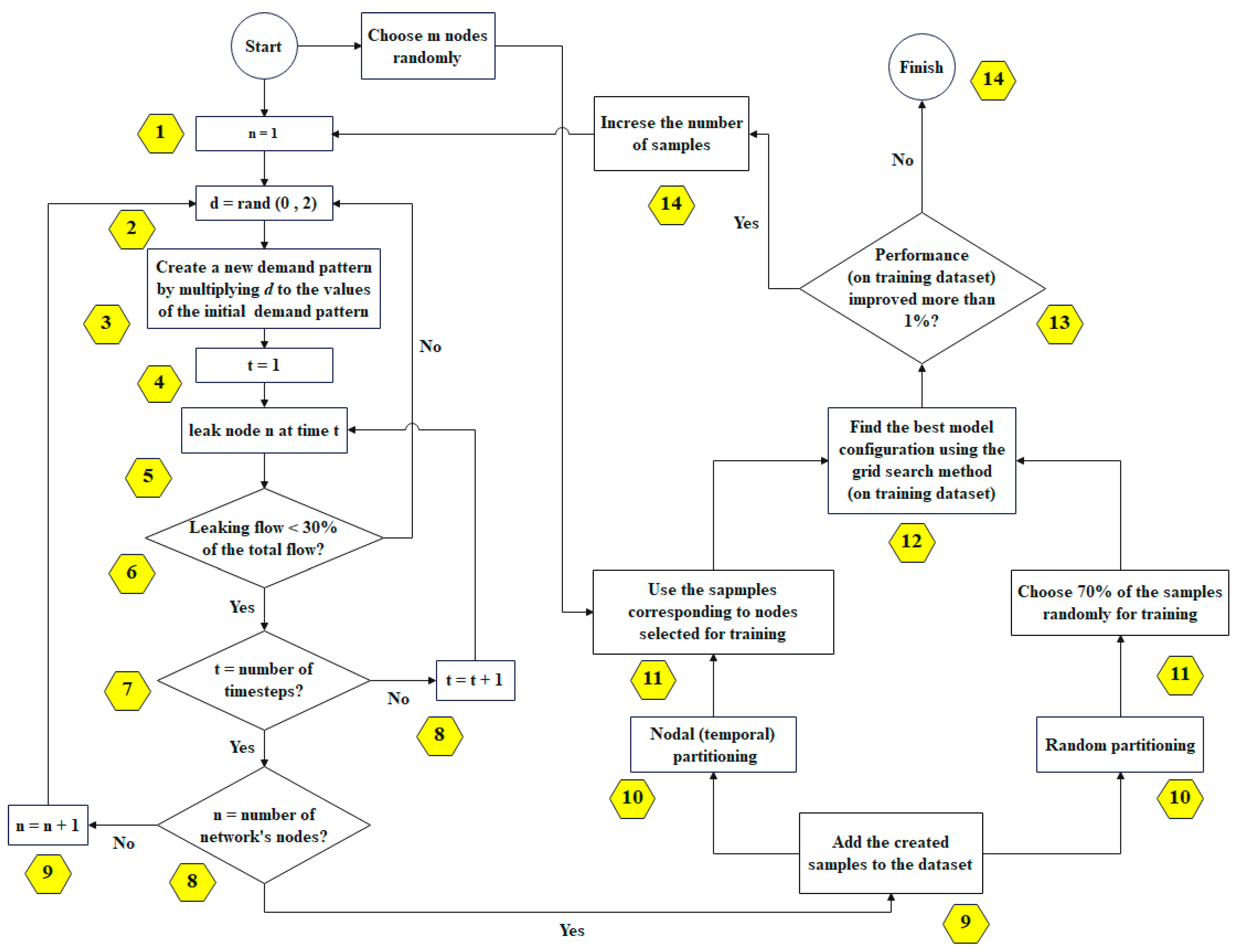
2.2. Data Simulation in EPANET
2.3. Feature and Target Engineering
2.4. Dataset Partitioning Strategy
2.5. ML Model Selection
2.6. Training
2.7. Evaluation Metrics
3. Results
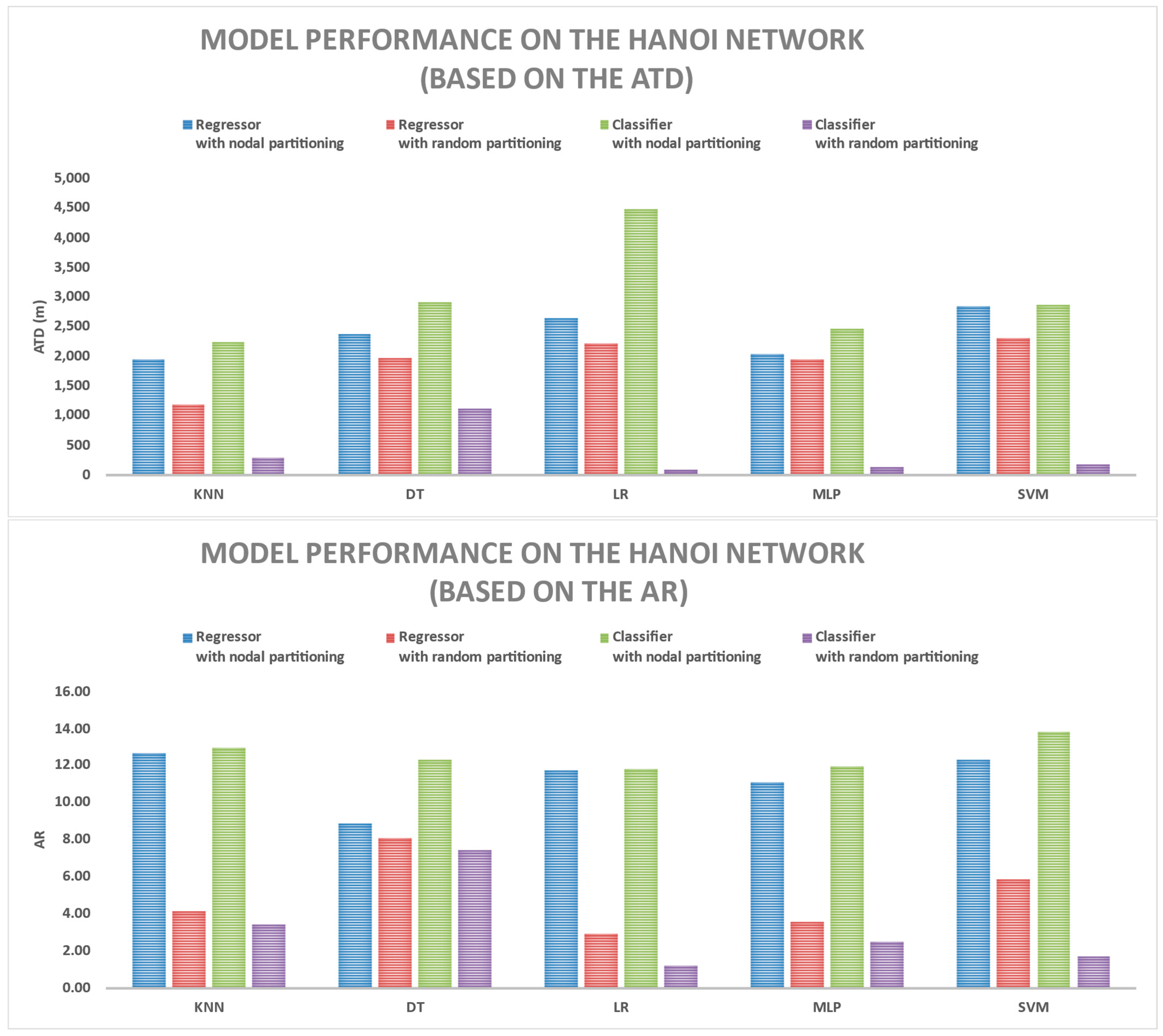
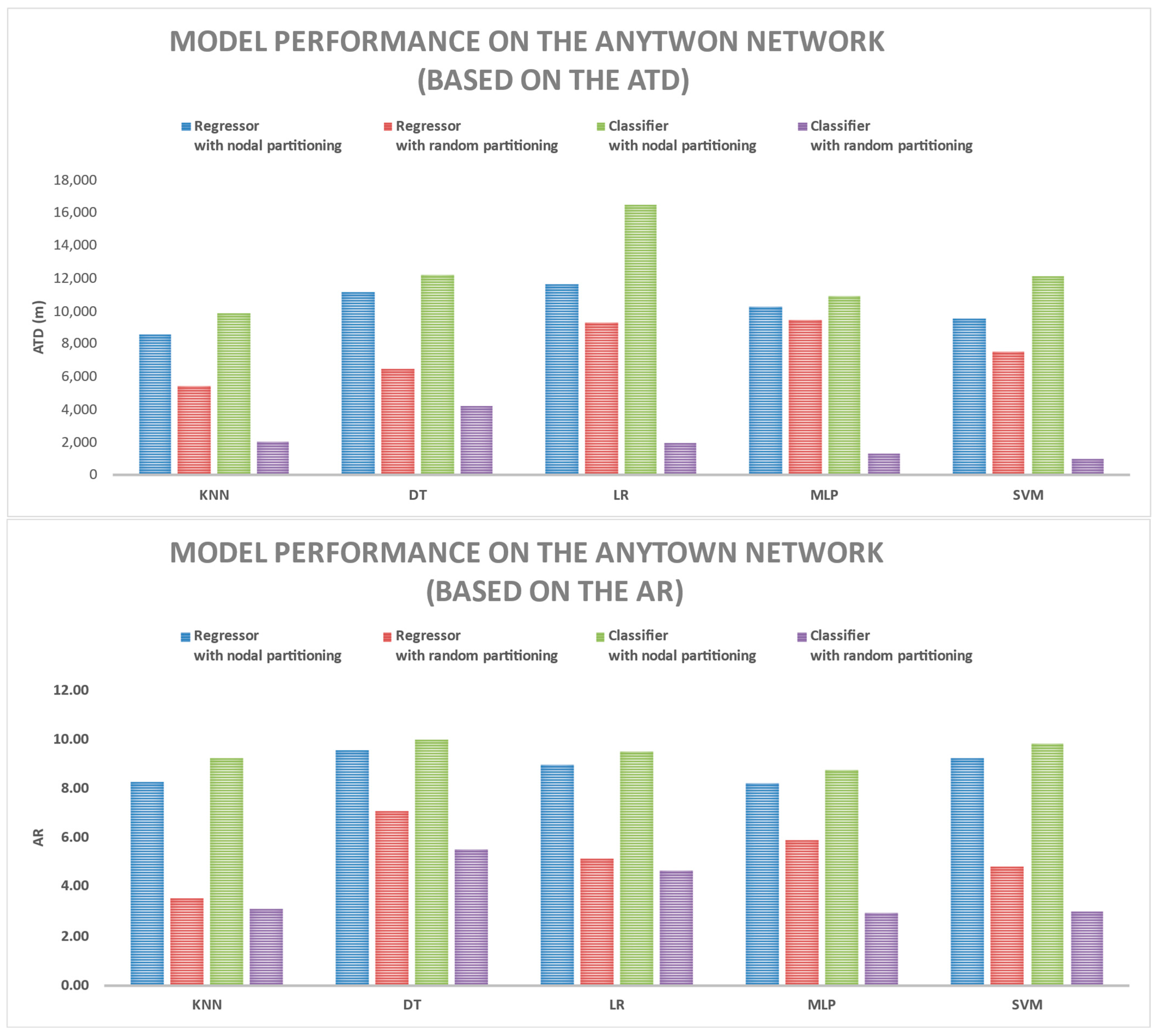
3.1. Comparing Various Models Based on ATD and AR Metrics
3.2. Comparing Results of Models on Train and Test Datasets
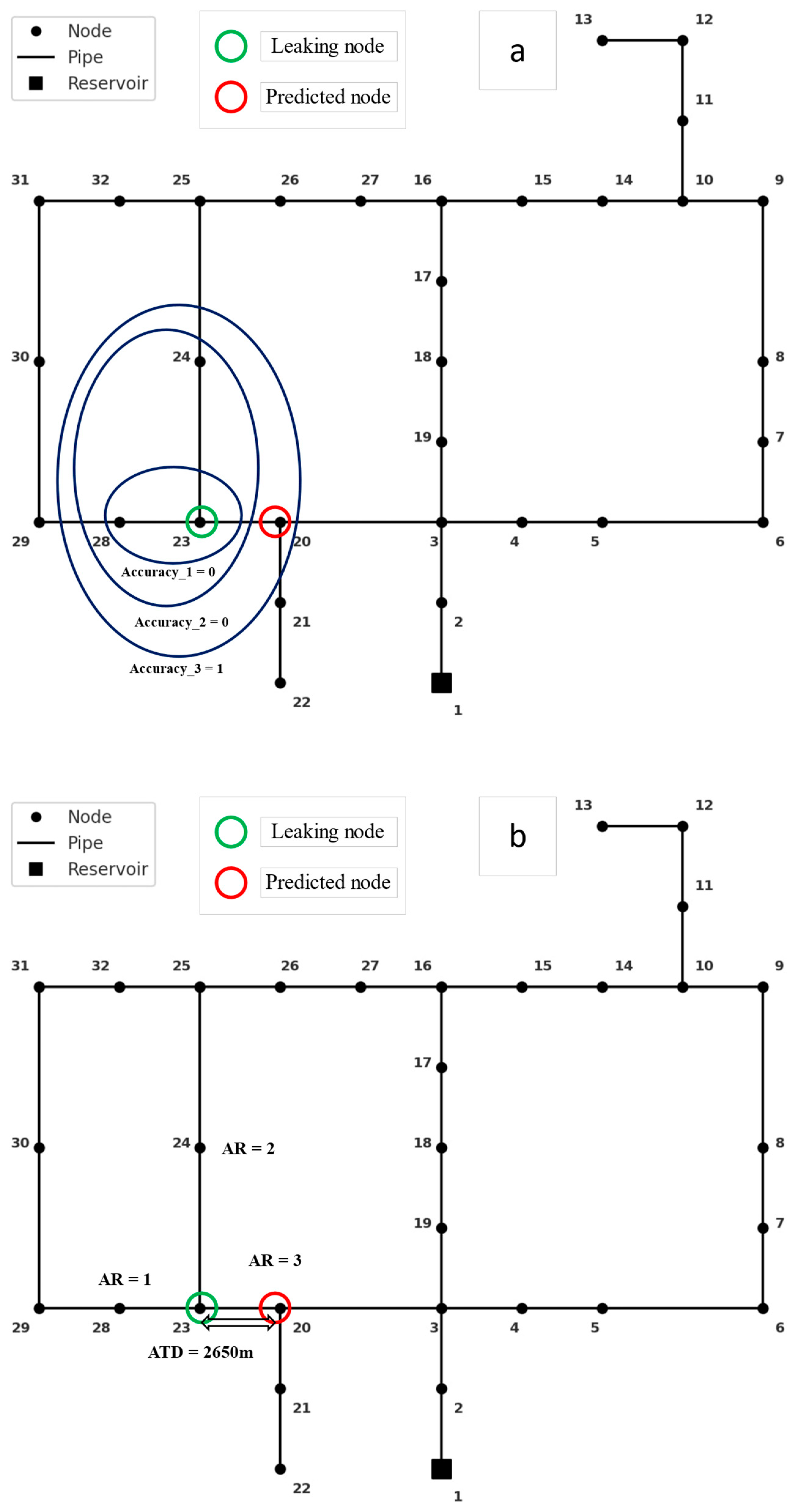
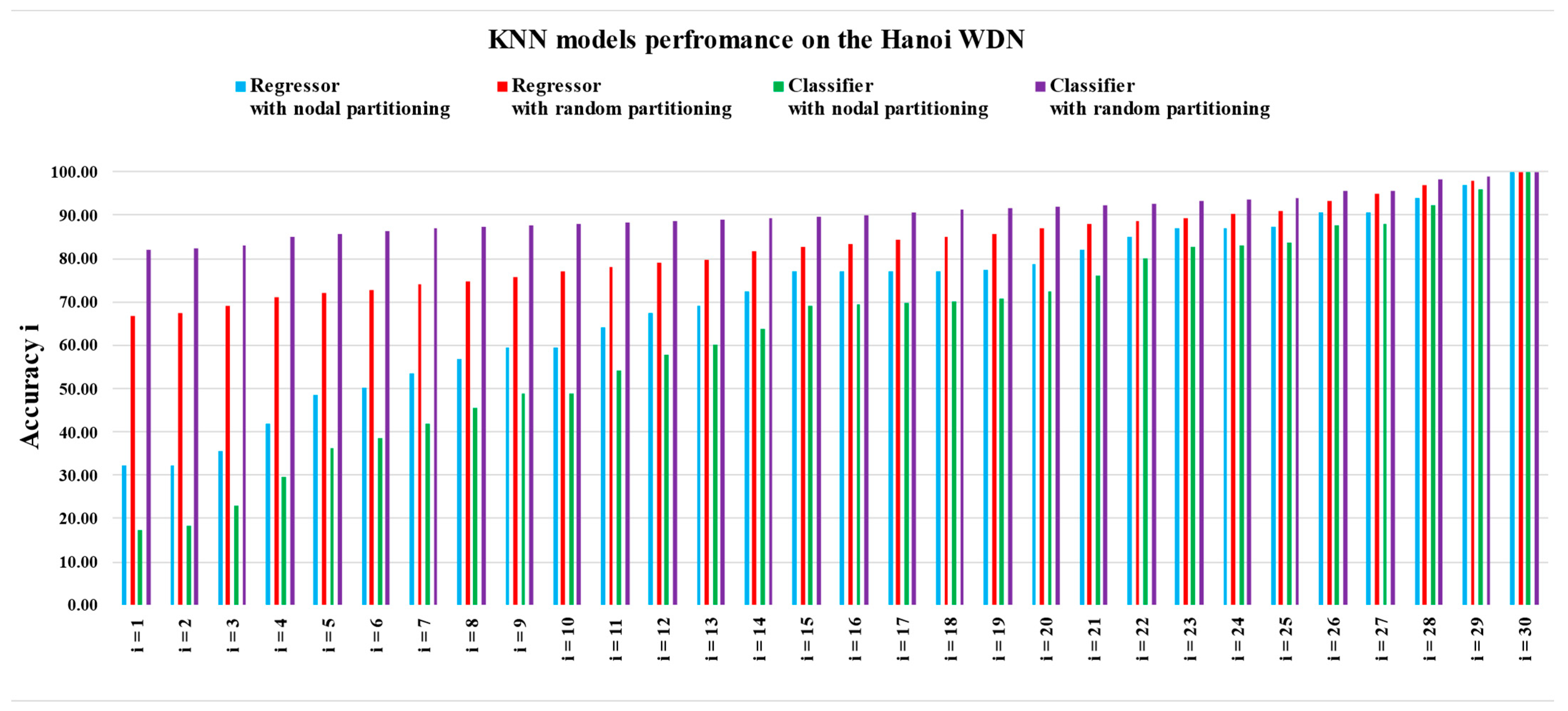
3.3. Comparing Various KNN Models Based on the Accuracyi Index
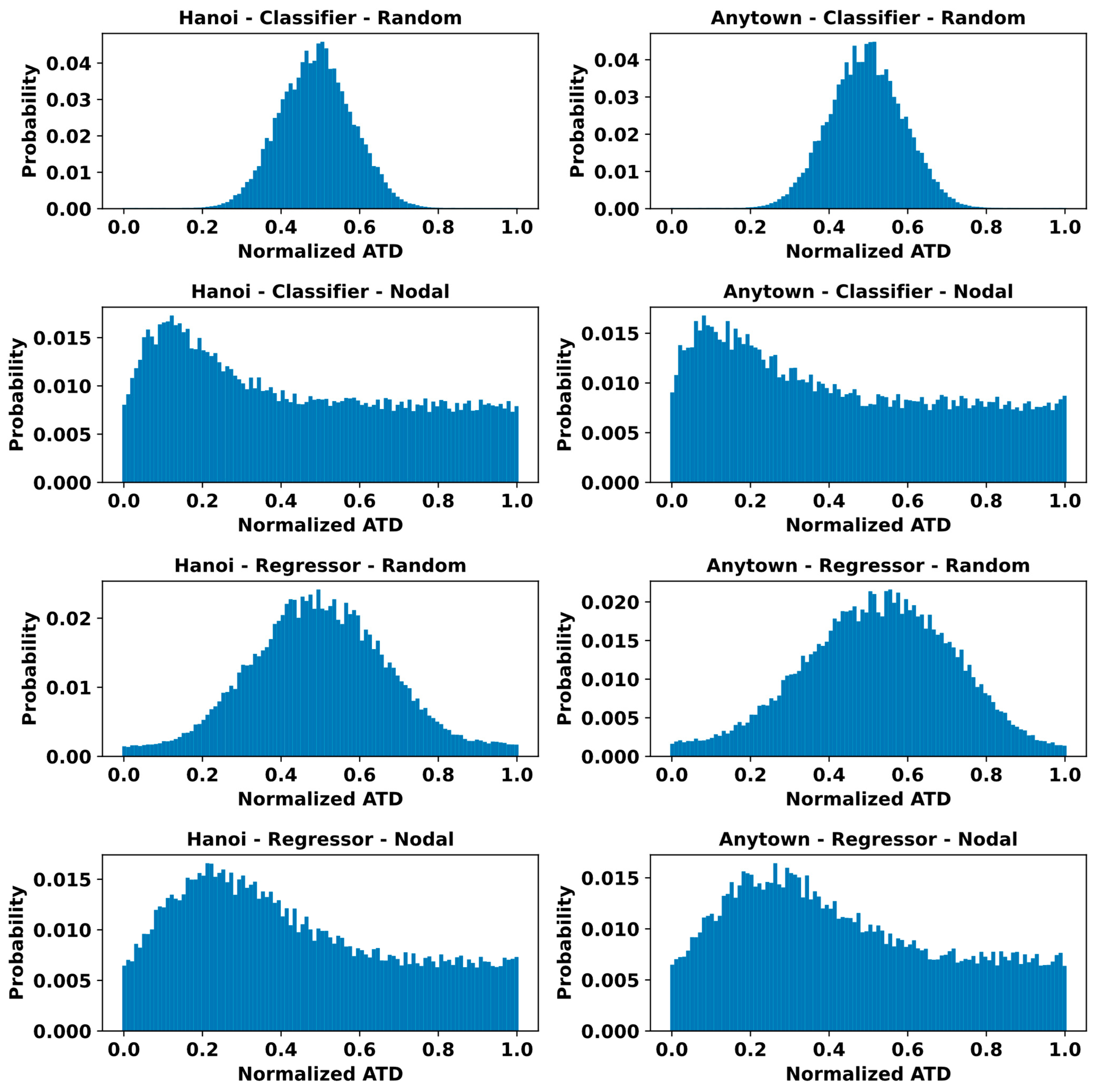
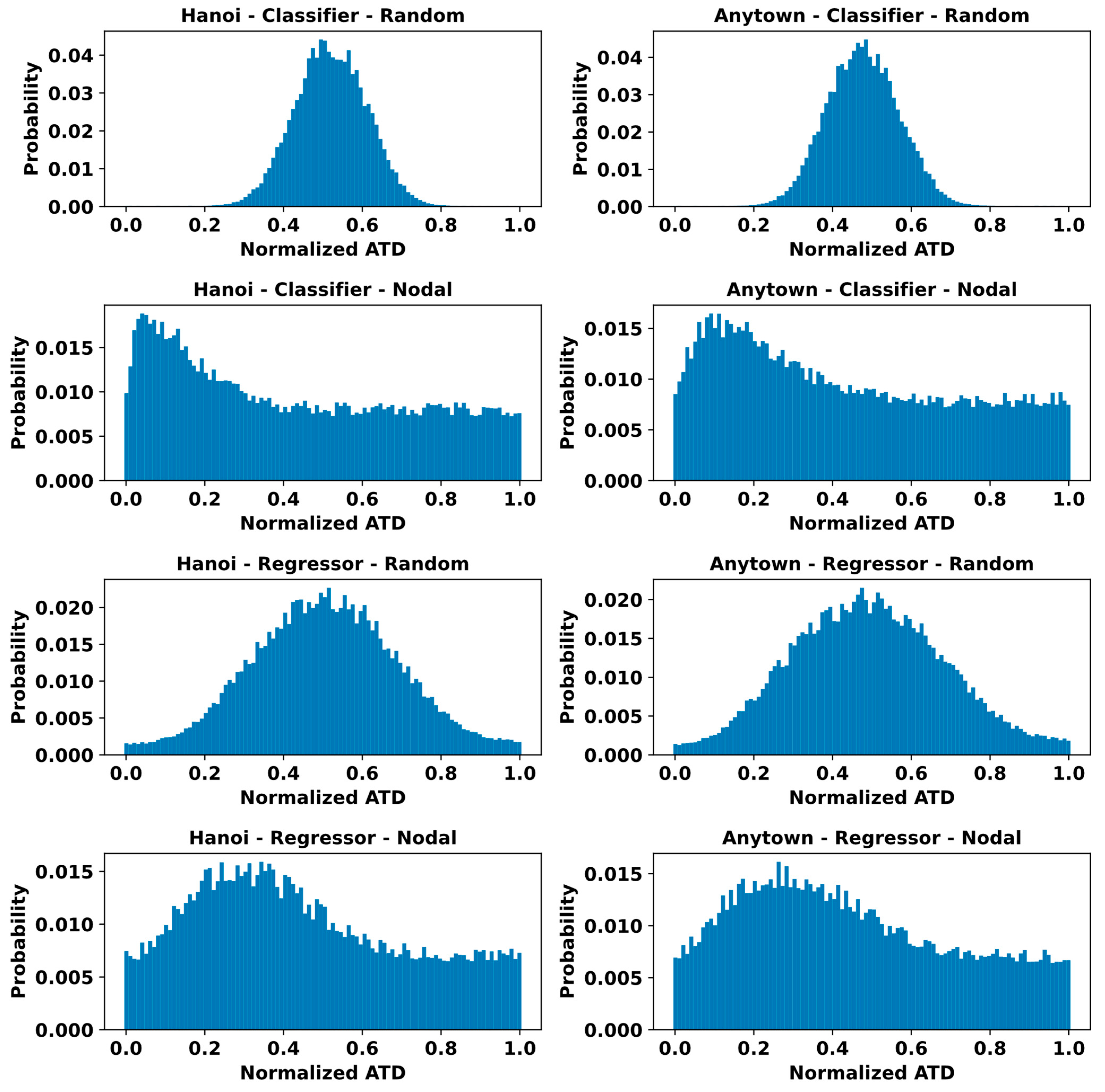
3.4. Assessing Error Distribution of the Models
3.5. Analysis of the Spatial Performance of the Models
4. Discussion and Conclusions
Author Contributions
Funding
Data Availability Statement
Conflicts of Interest
Appendix A

| Label | Diameter (mm) |
|---|---|
| 1 | 1016 |
| 2 | 1016 |
| 3 | 1016 |
| 4 | 1016 |
| 5 | 1016 |
| 6 | 1016 |
| 7 | 1016 |
| 8 | 1016 |
| 9 | 1016 |
| 10 | 762 |
| 11 | 609.6 |
| 12 | 609.6 |
| 13 | 508 |
| 14 | 406.4 |
| 15 | 304.8 |
| 16 | 304.8 |
| 17 | 406.4 |
| 18 | 508 |
| 19 | 508 |
| 20 | 1016 |
| 21 | 508 |
| 22 | 304.8 |
| 23 | 1016 |
| 24 | 762 |
| 25 | 762 |
| 26 | 508 |
| 27 | 304.8 |
| 28 | 304.8 |
| 29 | 406.4 |
| 30 | 406.4 |
| 31 | 304.8 |
| 32 | 304.8 |
| 33 | 406.4 |
| 34 | 1016 |
| Label | Base Demand (CMH) | Demand Pattern |
|---|---|---|
| 1 (Reservoir) | N.A. | N.A. |
| 2 | 890 | 1 |
| 3 | 850 | 1 |
| 4 | 130 | 1 |
| 5 | 725 | 1 |
| 6 | 1005 | 1 |
| 7 | 1350 | 1 |
| 8 | 550 | 1 |
| 9 | 525 | 1 |
| 10 | 525 | 1 |
| 11 | 500 | 4 |
| 12 | 560 | 4 |
| 13 | 940 | 4 |
| 14 | 615 | 1 |
| 15 | 280 | 1 |
| 16 | 310 | 5 |
| 17 | 865 | 5 |
| 18 | 1345 | 5 |
| 19 | 60 | 5 |
| 20 | 1275 | 2 |
| 21 | 930 | 4 |
| 22 | 485 | 4 |
| 23 | 1045 | 6 |
| 24 | 820 | 6 |
| 25 | 170 | 6 |
| 26 | 900 | 2 |
| 27 | 370 | 2 |
| 28 | 290 | 3 |
| 29 | 360 | 3 |
| 30 | 360 | 3 |
| 31 | 105 | 3 |
| 32 | 805 | 3 |
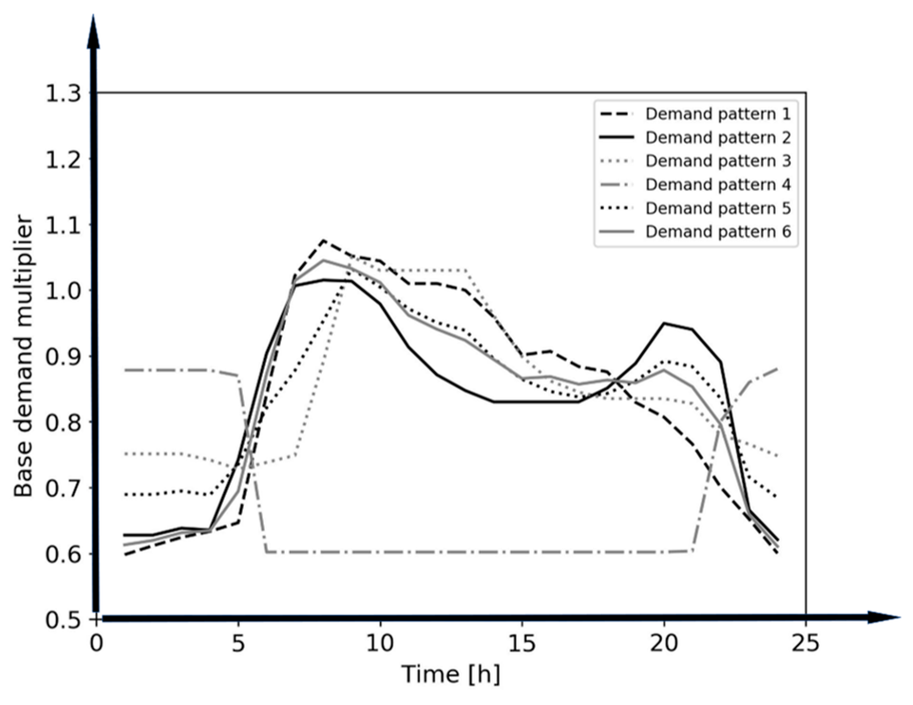
| Hour | Demand Multipliers |
|---|---|
| 0 | 1 |
| 1 | 1 |
| 2 | 1 |
| 3 | 0.9 |
| 4 | 0.9 |
| 5 | 0.9 |
| 6 | 0.7 |
| 7 | 0.7 |
| 8 | 0.7 |
| 9 | 0.6 |
| 10 | 0.6 |
| 11 | 0.6 |
| 12 | 1.2 |
| 13 | 1.2 |
| 14 | 1.2 |
| 15 | 1.3 |
| 16 | 1.3 |
| 17 | 1.3 |
| 18 | 1.2 |
| 19 | 1.2 |
| 20 | 1.2 |
| 21 | 1.1 |
| 22 | 1.1 |
| 23 | 1.1 |
| Model | Hyperparameters and Their Options |
|---|---|
| KNN | n-neighbors: {1, 2, 3, 4, 5, 6, 7, 8, 9, 10} |
| DT | criterion: {squared_error, friedman_mse, absolute_error, poisson} (for regressor) |
| criterion: {gini, entropy, log_loss} (for classifier) | |
| max_depth: {None, 1, 2, 5, 10, 20} | |
| min_samples_split: {2, 5, 10, 20} | |
| min_sample_leaf: {1, 2, 5, 10, 20} | |
| max_features: {1, 2, 5, 10, 20, 50, 100} | |
| LR | None |
| LoR (as an equivalent classifier for LR) | penalty: {None, L1, L2, elastic net} |
| C: {1, 2, 5, 10, 20, 50, 100} | |
| solver: {liblinear, newton-cg, lbfgs, sag, saga} | |
| MLP | hidden_layer_sizes: {(10), (20), (30), (40), (50), (60), (70), (80), (90), (100)} |
| activation: {relu, tanh, logistic} | |
| solver: {lbfgs, sgd, adam} | |
| learning_rate: {constant, adaptive} | |
| learning_rate_init: {0.01, 0.01, 0.001, 0.0001} | |
| SVM | C: {10,000, 20,000, 50,000, 100,000} |
| kernel: {linear, rbf, poly} | |
| degree: {2, 3} (for kernel: rbf) | |
| epsilon: {0.01, 0.02, 0.05, 0.1} (for regression} |
| Model | Results on Hanoi WDN | Results on Anytown WDN |
|---|---|---|
| KNN regressor with temporal partitioning | n-neighbors: 1 | n-neighbors: 1 |
| KNN regressor with random partitioning | n-neighbors: 2 | n-neighbors: 2 |
| KNN classifier with temporal partitioning | n-neighbors: 1 | n-neighbors: 1 |
| KNN classifier with random partitioning | n-neighbors: 2 | n-neighbors: 3 |
| DT regressor with temporal partitioning | criterion: absolute_error | criterion: poisson |
| max_depth: 10 | max_depth: 20 | |
| max_features: 20 | max_features: 10 | |
| min_sample_leaf: 1 | min_sample_leaf: 2 | |
| min_samples_split: 2 | min_samples_split: 5 | |
| DT regressor with random partitioning | criterion: friedman_mse | criterion: absolute_error |
| max_depth: None | max_depth: 20 | |
| max_features: 50 | max_features: 10 | |
| min_sample_leaf: 2 | min_sample_leaf: 1 | |
| min_samples_split: 5 | min_samples_split: 2 | |
| DT classifier with temporal partitioning | criterion: gini | criterion: log_loss |
| max_depth: 5 | max_depth: 10 | |
| max_features: 100 | max_features: 20 | |
| min_sample_leaf: 2 | min_sample_leaf: 1 | |
| min_samples_split: 2 | min_samples_split: 2 | |
| DT classifier with random partitioning | criterion: gini | criterion: gini |
| max_depth: None | max_depth: None | |
| max_features: 50 | max_features: 20 | |
| min_sample_leaf: 1 | min_sample_leaf: 1 | |
| min_samples_split: 2 | min_samples_split: 2 | |
| LR regressor with temporal partitioning | None | None |
| LR regressor with random partitioning | None | None |
| LoR classifier with temporal partitioning | C: 20 | C: 100 |
| penalty: L1 | penalty: L1 | |
| solver: liblinear | solver: liblinear | |
| LoR classifier with random partitioning | C: 50 | C: 100 |
| penalty: l1 | penalty: l1 | |
| solver: liblinear | solver: liblinear | |
| MLP regressor with temporal partitioning | activation: logistic | activation: logistic |
| hidden_layer_sizes: (70) | hidden_layer_sizes: (90) | |
| learning_rate: adaptive | learning_rate: adaptive | |
| learning_rate_init: 0.001 | learning_rate_init: 0.01 | |
| solver: lbfgs | solver: lbfgs | |
| MLP regressor with random partitioning | activation: relu | activation: relu |
| hidden_layer_sizes: (30) | hidden_layer_sizes: (30) | |
| learning_rate: constant | learning_rate: constant | |
| learning_rate_init: 0.0001 | learning_rate_init: 0.01 | |
| solver: lbfgs | solver: lbfgs | |
| MLP classifier with temporal partitioning | activation: relu | activation: logistic |
| hidden_layer_sizes: (10) | hidden_layer_sizes: (50) | |
| learning_rate: constant | learning_rate: constant | |
| learning_rate_init: 0.01 | learning_rate_init: 0.01 | |
| solver: adam | solver: lbfgs | |
| MLP classifier with random partitioning | activation: logistic | activation: relu |
| hidden_layer_sizes: (80) | hidden_layer_sizes: (30) | |
| learning_rate: constant | learning_rate: constant | |
| learning_rate_init: 0.0001 | learning_rate_init: 0.01 | |
| solver: lbfgs | solver: lbfgs | |
| SVM regressor with temporal partitioning | C: 20,000 | C: 100,000 |
| epsilon: 10 | epsilon: 100 | |
| kernel: rbf | kernel: rbf | |
| degree: N.A. | degree: N.A. | |
| SVM regressor with random partitioning | C: 100,000 | C: 50,000 |
| epsilon: 100 | epsilon: 100 | |
| kernel: rbf | kernel: rbf | |
| degree: N.A. | degree: N.A. | |
| SVM classifier with temporal partitioning | C: 10,000 | C: 100,000 |
| kernel: poly | kernel: poly | |
| degree: 2 | degree: 2 | |
| SVM classifier with random partitioning | C: 10,000 | C: 100,000 |
| kernel: poly | kernel: poly | |
| degree: 2 | degree: 2 |


References
- Sun, C.; Parellada, B.; Puig, V.; Cembrano, G. Leak localization in water distribution networks using pressure and data-driven classifier approach. Water 2020, 12, 54. [Google Scholar] [CrossRef]
- Fares, A.; Tijani, I.A.; Rui, Z.; Zayed, T. Leak detection in real water distribution networks based on acoustic emission and machine learning. Environ. Technol. 2023, 44, 3850–3866. [Google Scholar] [CrossRef] [PubMed]
- Daniel, I.; Pesantez, J.; Letzgus, S.; Khaksar Fasaee, M.A.; Alghamdi, F.; Berglund, E.; Mahinthakumar, G.; Cominola, A. A Sequential Pressure-Based Algorithm for Data-Driven Leakage Identification and Model-Based Localization in Water Distribution Networks. J. Water Resour. Plan. Manag. 2022, 148, 04022025. [Google Scholar] [CrossRef]
- Steffelbauer, D.B.; Deuerlein, J.; Gilbert, D.; Abraham, E.; Piller, O. Pressure-Leak Duality for Leak Detection and Localization in Water Distribution Systems. J. Water Resour. Plan. Manag. 2022, 148, 04021106. [Google Scholar] [CrossRef]
- Sanz, G.; Perez, R.; Escobet, A. Leakage localization in water networks using fuzzy logic. In Proceedings of the 2012 20th Mediterranean Conference on Control & Automation (MED), Barcelona, Spain, 3–6 July 2012; pp. 646–651. [Google Scholar] [CrossRef]
- Romero-Ben, L.; Alves, D.; Blesa, J.; Cembrano, G.; Puig, V.; Duviella, E. Leak detection and localization in water distribution networks: Review and perspective. Annu. Rev. Control 2023, 55, 392–419. [Google Scholar] [CrossRef]
- Burkart, N.; Huber, M.F. A Survey on the Explainability of Supervised Machine Learning. J. Artif. Intell. Res. 2021, 70, 245–317. [Google Scholar] [CrossRef]
- Soldevila, A.; Boracchi, G.; Roveri, M.; Tornil-Sin, S.; Puig, V. Leak detection and localization in water distribution networks by combining expert knowledge and data-driven models. Neural Comput. Appl. 2022, 34, 4759–4779. [Google Scholar] [CrossRef]
- Rossman, L.A. EPANET 2 USERS MANUAL. 2000. Available online: https://www.microimages.com/documentation/tutorials/epanet2usermanual.pdf (accessed on 29 April 2025).
- Pernot, P. Calibration in Machine Learning Uncertainty Quantification: Beyond consistency to target adaptivity. APL Mach. Learn. 2023, 1, 046121. [Google Scholar] [CrossRef]
- Braiek, H.B.; Khomh, F. On testing machine learning programs. J. Syst. Softw. 2020, 164, 110542. [Google Scholar] [CrossRef]
- Ramazi, P.; Haratian, A.; Meghdadi, M.; Mari Oriyad, A.; Lewis, M.A.; Maleki, Z.; Vega, R.; Wang, H.; Wishart, D.S.; Greiner, R. Accurate long-range forecasting of COVID-19 mortality in the USA. Sci. Rep. 2021, 11, 13822. [Google Scholar] [CrossRef]
- Ramazi, P.; Kunegel-Lion, M.; Greiner, R.; Lewis, M.A. Predicting insect outbreaks using machine learning: A mountain pine beetle case study. Ecol. Evol. 2021, 11, 13014–13028. [Google Scholar] [CrossRef] [PubMed]
- Sousa, C.; Calheiros, C.; Maria, A.; Geraldes, A.; Onukwube, C.U.; Aikhuele, D.O.; Sorooshian, S. Development of a Fault Detection and Localization Model for a Water Distribution Network. Appl. Sci. 2024, 14, 1620. [Google Scholar] [CrossRef]
- Mazaev, G.; Weyns, M.; Vancoillie, F.; Vaes, G.; Ongenae, F.; Van Hoecke, S. Probabilistic leak localization in water distribution networks using a hybrid data-driven and model-based approach. Water Supply 2023, 23, 162–178. [Google Scholar] [CrossRef]
- Tyagi, V.; Pandey, P.; Jain, S.; Ramachandran, P. A Two-Stage Model for Data-Driven Leakage Detection and Localization in Water Distribution Networks. Water 2023, 15, 2710. [Google Scholar] [CrossRef]
- Mazaev, G.; Weyns, M.; Moens, P.; Haest, P.J.; Vancoillie, F.; Vaes, G.; Debaenst, J.; Waroux, A.; Marlein, K.; Ongenae, F.; et al. A microservice architecture for leak localization in water distribution networks using hybrid AI. J. Hydroinformatics 2023, 25, 851–866. [Google Scholar] [CrossRef]
- Li, J.; Zheng, W.; Lu, C. An Accurate Leakage Localization Method for Water Supply Network Based on Deep Learning Network. Water Resour. Manag. 2022, 36, 2309–2325. [Google Scholar] [CrossRef]
- Lučin, I.; Lučin, B.; Čarija, Z.; Sikirica, A. Data-driven leak localization in urban water distribution networks using big data for random forest classifier. Mathematics 2021, 9, 672. [Google Scholar] [CrossRef]
- Mashhadi, N.; Shahrour, I.; Attoue, N.; El Khattabi, J.; Aljer, A. Use of machine learning for leak detection and localization in water distribution systems. Smart Cities 2021, 4, 1293–1315. [Google Scholar] [CrossRef]
- Soldevila, A.; Blesa, J.; Fernandez-Canti, R.M.; Tornil-Sin, S.; Puig, V. Data-driven approach for leak localization in water distribution networks using pressure sensors and spatial interpolation. Water 2019, 11, 1500. [Google Scholar] [CrossRef]
- Zhou, X.; Tang, Z.; Xu, W.; Meng, F.; Chu, X.; Xin, K.; Fu, G. Deep learning identifies accurate burst locations in water distribution networks. Water Res. 2019, 166, 115058. [Google Scholar] [CrossRef]
- Capelo, M.; Brentan, B.; Monteiro, L.; Covas, D. Near–real time burst location and sizing in water distribution systems using artificial neural networks. Water 2021, 13, 1841. [Google Scholar] [CrossRef]
- Javadiha, M.; Blesa, J.; Soldevila, A.; Puig, V. Leak localization in water distribution networks using deep learning. In Proceedings of the 2019 6th International Conference on Control, Decision and Information Technologies (CoDIT), Paris, France, 23–26 April 2019. [Google Scholar] [CrossRef]
- Fujiwara, O.; Khang, D.B. A two-phase decomposition method for optimal design of looped water distribution networks. Water Resour. Res. 1990, 26, 539–549. [Google Scholar] [CrossRef]
- Geem, Z.W. Optimal cost design of water distribution networks using harmony search. Eng. Optim. 2006, 38, 259–277. [Google Scholar] [CrossRef]
- Walski, T.M.; Brill, E.D.; Gessler, J.; Goulter, I.C.; Jeppson, R.M.; Lansey, K.; Lee, H.; Liebman, J.C.; Mays, L.; Morgan, D.R.; et al. Battle of the Network Models: Epilogue. J. Water Resour. Plan. Manag. 1987, 113, 191–203. [Google Scholar] [CrossRef]
- Xu, J.; Wang, H.; Rao, J.; Wang, J. Zone scheduling optimization of pumps in water distribution networks with deep reinforcement learning and knowledge-assisted learning. Soft Comput. 2021, 25, 14757–14767. [Google Scholar] [CrossRef]
- Yang, L.; Shami, A. On hyperparameter optimization of machine learning algorithms: Theory and practice. Neurocomputing 2020, 415, 295–316. [Google Scholar] [CrossRef]
- Halabaku, E.; Bytyçi, E. Overfitting in Machine Learning: A Comparative Analysis of Decision Trees and Random Forests. Intell. Autom. Soft Comput. 2024, 39, 987–1006. [Google Scholar] [CrossRef]
- Wong, T.T.; Yeh, P.Y. Reliable Accuracy Estimates from k-Fold Cross Validation. IEEE Trans. Knowl. Data Eng. 2020, 32, 1586–1594. [Google Scholar] [CrossRef]
- Pereira, R.B.; Plastino, A.; Zadrozny, B.; Merschmann, L.H.C. Correlation analysis of performance measures for multi-label classification. Inf. Process. Manag. 2018, 54, 359–369. [Google Scholar] [CrossRef]


| Work | The Input | The Output | Trained Classifiers | Case Studies | Results |
|---|---|---|---|---|---|
| [15] | pressure at nodes | label of the leaking node | logistic regression (LoR) | a district-metered area in Belgium | Average topological distance (ATD) = 0.18 to 4.96 km |
| [16] | flow of some pipes and pressure at some nodes | label of the leaking node | LoR | Hanoi | Accuracy = 91% |
| Net3 | Accuracy = 79% | ||||
| C-Town | Accuracy = 30% | ||||
| [17] | pressure at nodes | label of the leaking node | elastic-net LoR | a district-metered area in Belgium | ATD = 0.17 to 1.2 km |
| [18] | pressure at some nodes | label of the leaking pipe | ResNet | Anytown | Accuracy = 94% |
| Net3 | Accuracy = 91% | ||||
| [8] | flow of pipes | label of the leaking area | KNN | Barcelona WDN | Accuracy = 80% |
| [19] | residual pressures at some node | label of the leaking node | Random forest (RF) | Hanoi | Accuracy = 100% |
| [20] | flow of some pipes and residual pressure at some nodes | label of the leaking node | LoR | Lille University network | Accuracy = 100% |
| [21] | residual pressure at nodes | label of the leaking node | KNN | Hanoi | ATD = 2.3 nodes |
| [22] | pressure at some nodes | label of the leaking pipe | ANN | Anytown | Accuracy = 100% |
| Model Name | Model Type | Partitioning Type | Hanoi Train | Hanoi Test | Anytown Train | Anytown Test |
|---|---|---|---|---|---|---|
| KNN | Regressor | Nodal | 1895 | 1951 | 8306 | 8553 |
| Regressor | Random | 1154 | 1180 | 5338 | 5461 | |
| Classifier | Nodal | 810 | 2239 | 3587 | 9919 | |
| Classifier | Random | 272 | 277 | 2043 | 2087 | |
| DT | Regressor | Nodal | 2266 | 2367 | 10,693 | 11,168 |
| Regressor | Random | 1872 | 1970 | 6201 | 6526 | |
| Classifier | Nodal | 1011 | 2905 | 4259 | 12,241 | |
| Classifier | Random | 1086 | 1121 | 4121 | 4255 | |
| LR | Regressor | Nodal | 2597 | 2649 | 11,425 | 11,654 |
| Regressor | Random | 2173 | 2212 | 9178 | 9341 | |
| Classifier | Nodal | 2012 | 4481 | 7423 | 16,528 | |
| Classifier | Random | 86 | 89 | 1958 | 2005 | |
| MLP | Regressor | Nodal | 1988 | 2029 | 10,092 | 10,297 |
| Regressor | Random | 1929 | 1939 | 9445 | 9493 | |
| Classifier | Nodal | 1170 | 2473 | 5173 | 10,930 | |
| Classifier | Random | 138 | 139 | 1353 | 1355 | |
| SVM | Regressor | Nodal | 2778 | 2846 | 9326 | 9555 |
| Regressor | Random | 2245 | 2311 | 7300 | 7517 | |
| Classifier | Nodal | 923 | 2874 | 3908 | 12,174 | |
| Classifier | Random | 167 | 171 | 1009 | 1033 |
| Model Name | Model Type | Partitioning Type | Hanoi Train | Hanoi Test | Anytown Train | Anytown Test |
|---|---|---|---|---|---|---|
| KNN | Regressor | Nodal | 12.33 | 12.70 | 8.02 | 8.26 |
| Regressor | Random | 4.03 | 4.12 | 3.47 | 3.55 | |
| Classifier | Nodal | 4.70 | 12.99 | 3.34 | 9.23 | |
| Classifier | Random | 3.35 | 3.42 | 3.06 | 3.13 | |
| DT | Regressor | Nodal | 8.48 | 8.86 | 9.16 | 9.57 |
| Regressor | Random | 7.71 | 8.12 | 6.74 | 7.09 | |
| Classifier | Nodal | 4.29 | 12.33 | 3.48 | 10.01 | |
| Classifier | Random | 7.17 | 7.40 | 5.35 | 5.53 | |
| LR | Regressor | Nodal | 11.49 | 11.73 | 8.81 | 8.99 |
| Regressor | Random | 2.88 | 2.93 | 5.07 | 5.16 | |
| Classifier | Nodal | 5.31 | 11.82 | 4.26 | 9.49 | |
| Classifier | Random | 1.13 | 1.15 | 4.53 | 4.64 | |
| MLP | Regressor | Nodal | 10.88 | 11.10 | 8.05 | 8.22 |
| Regressor | Random | 3.53 | 3.55 | 5.90 | 5.93 | |
| Classifier | Nodal | 5.67 | 11.99 | 4.13 | 8.73 | |
| Classifier | Random | 2.46 | 2.47 | 2.96 | 2.97 | |
| SVM | Regressor | Nodal | 12.03 | 12.33 | 9.03 | 9.25 |
| Regressor | Random | 5.71 | 5.88 | 4.70 | 4.84 | |
| Classifier | Nodal | 4.43 | 13.81 | 3.15 | 9.83 | |
| Classifier | Random | 1.68 | 1.72 | 2.94 | 3.01 |
Disclaimer/Publisher’s Note: The statements, opinions and data contained in all publications are solely those of the individual author(s) and contributor(s) and not of MDPI and/or the editor(s). MDPI and/or the editor(s) disclaim responsibility for any injury to people or property resulting from any ideas, methods, instructions or products referred to in the content. |
© 2025 by the authors. Licensee MDPI, Basel, Switzerland. This article is an open access article distributed under the terms and conditions of the Creative Commons Attribution (CC BY) license (https://creativecommons.org/licenses/by/4.0/).
Share and Cite
Ajoodani, A.; Nazif, S.; Ramazi, P. Towards a Realistic Data-Driven Leak Localization in Water Distribution Networks. Water 2025, 17, 1988. https://doi.org/10.3390/w17131988
Ajoodani A, Nazif S, Ramazi P. Towards a Realistic Data-Driven Leak Localization in Water Distribution Networks. Water. 2025; 17(13):1988. https://doi.org/10.3390/w17131988
Chicago/Turabian StyleAjoodani, Arvin, Sara Nazif, and Pouria Ramazi. 2025. "Towards a Realistic Data-Driven Leak Localization in Water Distribution Networks" Water 17, no. 13: 1988. https://doi.org/10.3390/w17131988
APA StyleAjoodani, A., Nazif, S., & Ramazi, P. (2025). Towards a Realistic Data-Driven Leak Localization in Water Distribution Networks. Water, 17(13), 1988. https://doi.org/10.3390/w17131988