
Interdisciplinary Evaluation of the Săpânța River and Groundwater Quality: Linking Hydrological Data and Vegetative Bioindicators


Abstract
1. Introduction
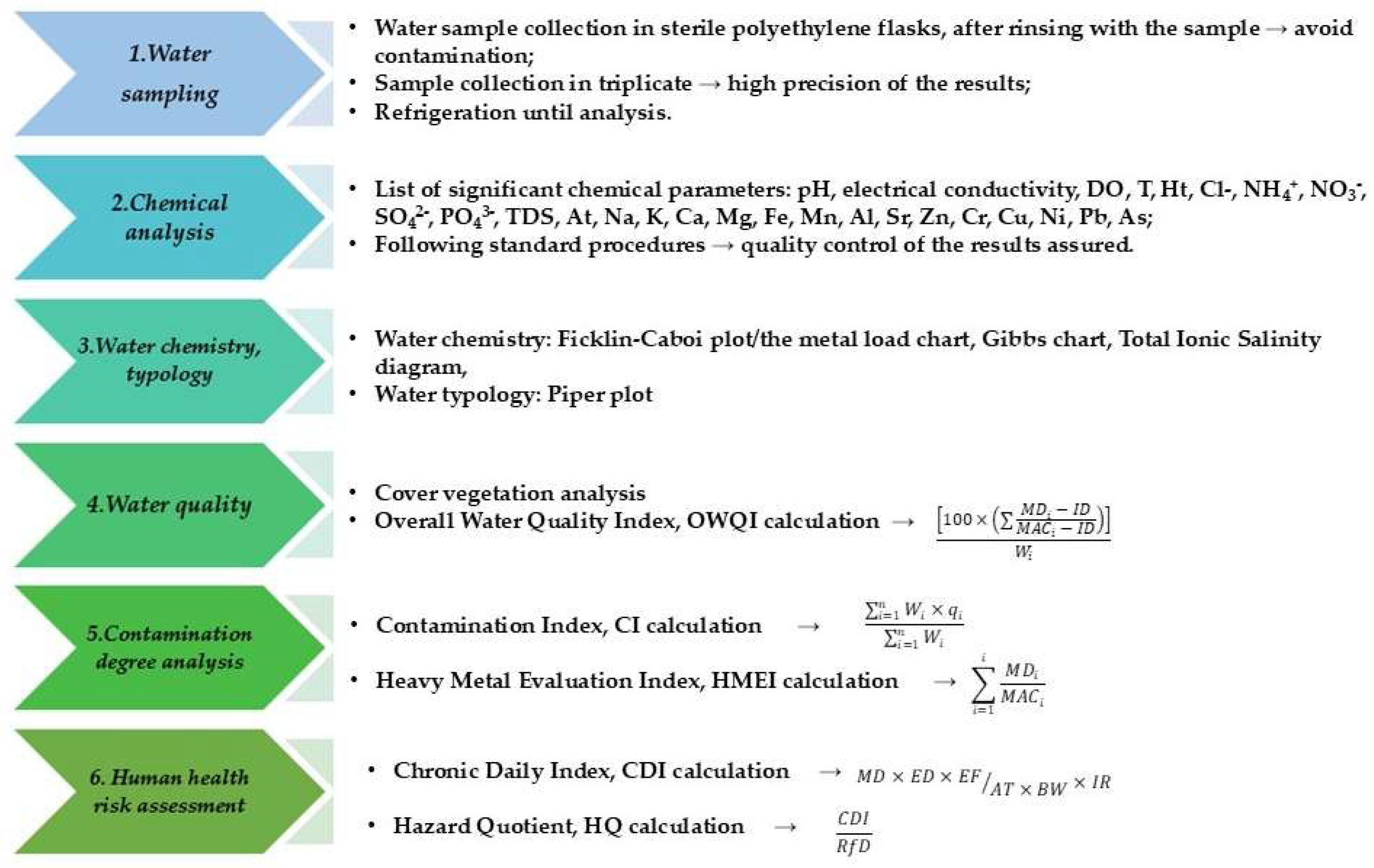
2. Materials and Methods
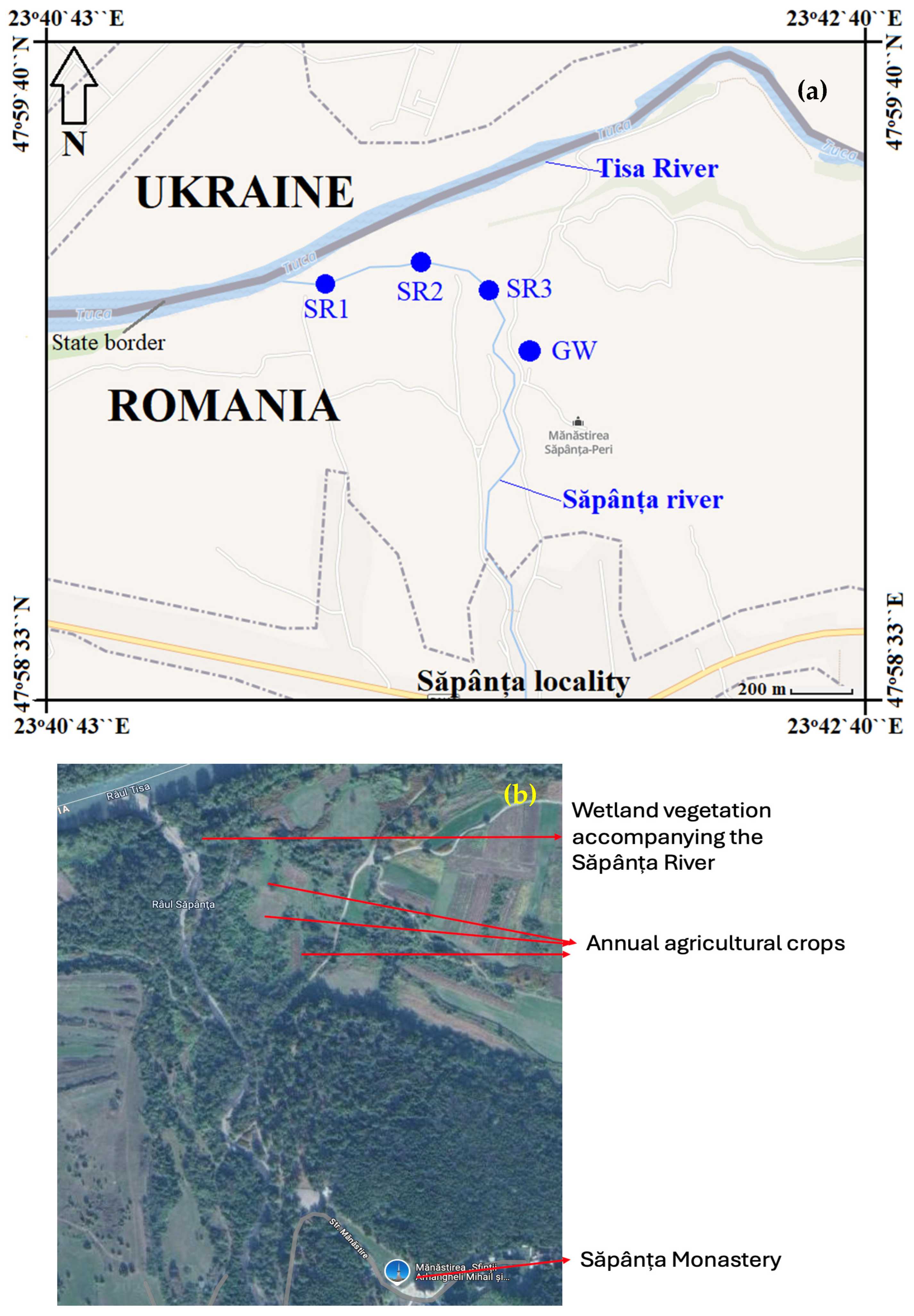
2.1. Study Area and Sampling
2.2. Water Quality Analysis
2.3. Water Typology
2.4. Potential Contamination Degree Evaluation
2.5. Human Health Risk Assessment of Toxins
3. Results and Discussion
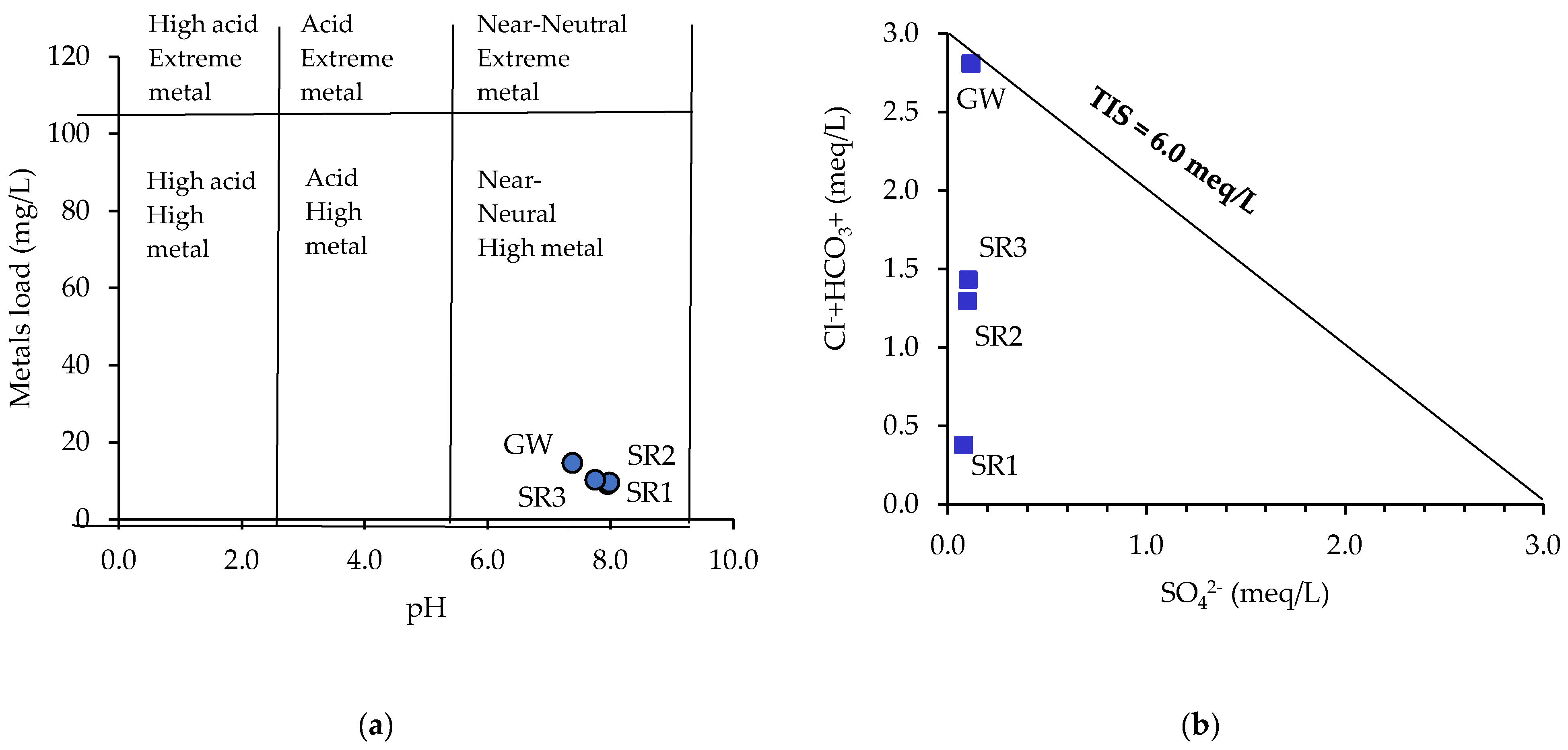
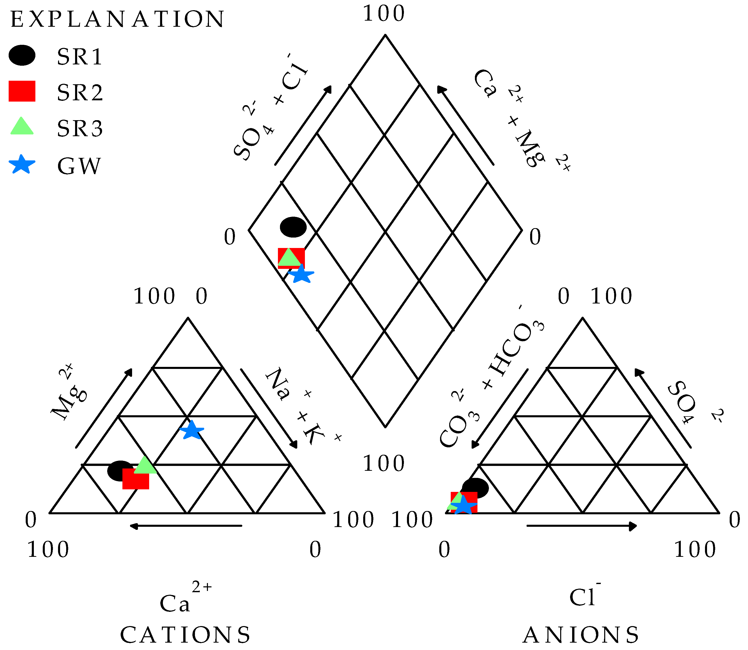
3.1. Analysis of Water Chemistry

| SI | SR1 | SR2 | SR3 | GW | Mean | Median | Min | Max | SD | Errors | MAC * | |
|---|---|---|---|---|---|---|---|---|---|---|---|---|
| EC | μS/cm | 50.0 ± 4.8 | 46.2 ± 4.5 | 43.3 ± 4.1 | 255 ± 23 | 98.6 | 48.1 | 43.3 | 255 | 104 | ±8.3 | 250 |
| pH | - | 7.95 ± 0.77 | 7.98 ± 0.78 | 7.75 ± 0.63 | 7.38 ± 0.21 | 7.77 | 7.85 | 7.99 | 7.98 | 0.28 | ±1.15 | 6.5–9.5 |
| DO | mg/L | 9.26 ± 0.89 | 8.69 ± 0.72 | 8.55 ± 0.81 | 7.99 ± 0.68 | 8.63 | 8.62 | 1.09 | 9.26 | 0.52 | ±1.10 | - |
| T | NTU | 2.15 ± 0.19 | 5.52 ± 0.47 | 3.16 ± 0.30 | 1.09 ± 0.09 | 2.98 | 2.66 | 1.86 | 5.52 | 1.89 | ±0.25 | <5 |
| Ht | °g | 2.45 ± 0.15 | 1.86 ± 0.12 | 2.78 ± 0.22 | 11.55 ± 0.96 | 4.66 | 2.62 | 1.01 | 11.55 | 4.61 | ±0.19 | >5 |
| Cl− | mg/L | 1.01 ± 0.88 | 2.75 ± 0.16 | 1.88 ± 0.16 | 5.65 ± 0.53 | 2.82 | 2.32 | 0.045 | 5.65 | 2.01 | ±0.08 | 250 |
| NH4+ | mg/L | 0.045 ± 0.004 | 0.057 ± 0.005 | 0.053 ± 0.005 | 0.066 ± 0.006 | 0.055 | 0.055 | 2.23 | 0.066 | 0.009 | ±0.002 | 0.5 |
| NO3− | mg/L | 2.23 ± 0.17 | 2.76 ± 0.20 | 2.88 ± 0.24 | 5.52 ± 0.49 | 3.35 | 2.82 | 3.84 | 5.52 | 1.48 | ±0.39 | 50 |
| SO42− | mg/L | 3.84 ± 0.29 | 4.68 ± 0.33 | 4.89 ± 0.41 | 5.45 ± 0.26 | 4.72 | 4.79 | 3.84 | 5.45 | 0.67 | ±0.42 | 250 |
| PO43− | mg/L | 0.02 ± 0.001 | 0.04 ± 0.002 | 0.03 ± 0.001 | 0.03 ± 0.002 | 0.03 | 0.03 | 0.02 | 0.04 | 0.008 | ±0.001 | 0.4 |
| TDS | mg/L | 44.2 ± 4.2 | 47.2 ± 3.9 | 53.5 ± 5.1 | 62.9 ± 5.9 | 52.0 | 50.6 | 44.2 | 62.9 | 8.3 | ±4.2 | - |
| At | mmol/L | 0.35 ± 0.02 | 1.22 ± 0.11 | 1.38 ± 0.09 | 2.65 ± 0.19 | 1.40 | 1.30 | 0.35 | 2.65 | 0.95 | ±0.05 | - |
| Metals | SI | SR1 | SR2 | SR3 | GW | Mean | Median | Min | Max | SD | Errors | MAC * |
|---|---|---|---|---|---|---|---|---|---|---|---|---|
| Na | mg/L | 1.22 ± 0.11 | 1.45 ± 0.14 | 1.56 ± 0.15 | 3.82 ± 0.35 | 2.01 | 1.51 | 1.22 | 3.82 | 1.21 | 0.17 | 200 |
| K | mg/L | 0.76 ± 0.05 | 1.63 ± 0.12 | 1.83 ± 0.16 | 2.63 ± 0.19 | 1.71 | 1.73 | 0.76 | 2.63 | 0.77 | 0.14 | 10 |
| Ca | mg/L | 5.91 ± 0.48 | 5.47 ± 0.51 | 5.33 ± 0.46 | 4.22 ± 0.39 | 5.23 | 5.40 | 4.22 | 5.91 | 0.72 | 0.50 | 100 |
| Mg | mg/L | 1.22 ± 0.10 | 0.94 ± 0.77 | 1.44 ± 0.12 | 3.89 ± 0.27 | 1.87 | 1.33 | 0.94 | 3.89 | 1.36 | 0.16 | 50 |
| Fe | μg/L | 5.52 ± 0.46 | 4.22 ± 0.38 | 5.15 ± 0.47 | 5.92 ± 0.52 | 5.20 | 5.34 | 4.22 | 5.92 | 0.73 | 0.52 | 20 |
| Mn | μg/L | 7.71 ± 0.68 | 7.16 ± 0.70 | 7.03 ± 0.66 | 6.88 ± 0.61 | 7.20 | 7.10 | 6.88 | 7.71 | 0.36 | 0.68 | 50 |
| Al | μg/L | 16.8 ± 0.12 | 17.3 ± 0.08 | 17.9 ± 0.12 | 18.5 ± 0.08 | 17.6 | 17.6 | 16.8 | 18.5 | 0.74 | 1.69 | 200 |
| Sr | μg/L | 19.5 ± 0.15 | 23.2 ± 0.20 | 27.5 ± 0.21 | 31.1 ± 0.26 | 25.3 | 25.4 | 19.5 | 31.1 | 5.05 | 2.49 | 7000 |
| Zn | μg/L | 11.1 ± 0.09 | 14.3 ± 0.08 | 13.5 ± 0.07 | 34.7 ± 0.15 | 18.4 | 13.9 | 11.1 | 34.7 | 10.9 | 1.80 | 5000 |
| Cr | μg/L | 0.88 ± 0.06 | 0.95 ± 0.07 | 0.99 ± 0.08 | 1.23 ± 0.09 | 1.01 | 0.97 | 0.88 | 1.23 | 0.15 | 0.09 | 50 |
| Cu | μg/L | 2.71 ± 0.12 | 3.41 ± 0.28 | 3.22 ± 0.25 | 5.22 ± 0.43 | 3.64 | 3.32 | 2.71 | 5.22 | 1.09 | 0.35 | 100 |
| Ni | μg/L | 0.88 ± 0.05 | 1.07 ± 0.07 | 1.25 ± 0.05 | 1.37 ± 0.02 | 1.14 | 1.16 | 0.88 | 1.37 | 0.21 | 0.10 | 20 |
| Pb | μg/L | 1.11 ± 0.02 | 1.37 ± 0.05 | 1.55 ± 0.09 | 1.84 ± 0.06 | 1.47 | 1.46 | 1.11 | 1.84 | 0.31 | 0.14 | 10 |
| As | μg/L | 0.39 ± 0.012 | 0.52 ± 0.02 | 0.49 ± 0.03 | 0.22 ± 0.01 | 0.41 | 0.44 | 0.22 | 0.52 | 0.14 | 0.04 | 10 |
3.2. Analysis of Water Quality and Contamination Level
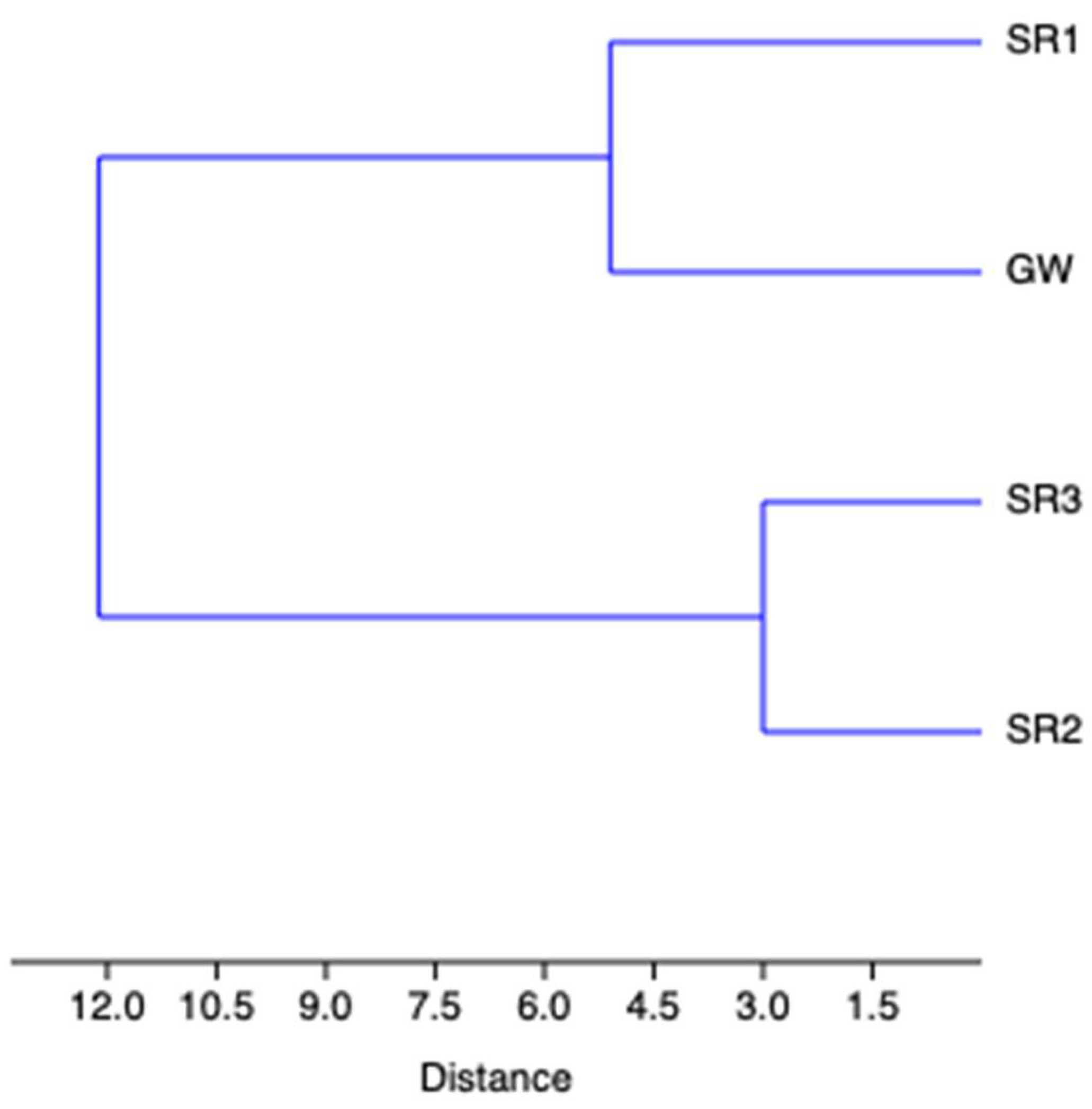
3.3. Water Quality Based on Vegetation Cover near Săpânța River
3.4. Health Risk Assessment for Toxins
4. Conclusions
Supplementary Materials
Author Contributions
Funding
Data Availability Statement
Conflicts of Interest
References
- Nidhi, J.; Yevatikar, R.; Raxamwar, S.T. Comparative study of physico-chemical parameters and water quality index of river. Mater. Today Proc. 2021, 60, 859–867. [Google Scholar]
- Unech, R.; Bibi, C.; Welch, B.; Jamilson, H.; Sundaranar, K. Assessement of the bacteorogical quality and physico-chemical parameters of household water sources. Int. J. Ecol. Sci. Environ. Engin. 2020, 6, 14–17. [Google Scholar]
- Dippong, T.; Hoaghia, M.A.; Senila, M. Appraisal of heavy metal pollution in alluvial aquifers. Study case on the protected area of Ronișoara Forest, Romania. Ecol. Indic. 2022, 143, 109347. [Google Scholar] [CrossRef]
- Dippong, T.; Mihali, C.; Marian, M.; Mare Rosca, O.; Resz, M.A. Correlations between chemical, hydrological and biotic factors in rivers from the protected area of Tisa Superioară, Romania. Process Saf. Environ. Prot. 2023, 176, 40–55. [Google Scholar] [CrossRef]
- Horvat, M.; Horvat, Z. Long term sediment transport simulaţion of the Danube, Sava and Tisa rivers. Int. J. Sediment Res. 2020, 35, 550–561. [Google Scholar] [CrossRef]
- Dippong, T.; Senila, M.; Cadar, O.; Resz, M.A. Assessment of the heavy metal pollution degree and potential health risk implications in lakes and fish from northern Romania. J. Environ. Chem. Eng. 2024, 12, 112217. [Google Scholar] [CrossRef]
- Sanja, M.; Sakan, M.; Ninod, M.; Dordevic, S. Trace element study in Tisa river and Danube alluvial sediment in Serbia. Int. J. Sediment Res. 2013, 28, 234–245. [Google Scholar]
- Dippong, T.; Resz, M.A. Heavy metal contamination assessment and potential human health risk of water quality of lakes situated in the protected area of Tisa, Romania. Heliyon 2024, 10, e28860. [Google Scholar] [CrossRef]
- Dippong, T.; Resz, M.A.; Tănăselia, C.; Cadar, O. Assessing microbiological and heavy metal pollution in surface waters associated with potential human health risk assessment at fish ingestion exposure. J. Hazard. Mater. 2024, 476, 135187. [Google Scholar] [CrossRef]
- Roberto, C.G. Freshwater Biodiversity: A Review of Local and Global Threats. Int. J. Environ. Stud. 2016, 73, 887–904. [Google Scholar]
- Geist, J. Integrative freshwater ecology and biodiversity conservation. Ecol. Ind. 2011, 11, 1507–1516. [Google Scholar]
- Shatwell, T.; Thiery, W.; Kirillin, G. Future projections of temperature and mixing regime of European temperate lakes. Hydrol. Earth Syst. Sci. 2019, 23, 1533–1551. [Google Scholar] [CrossRef]
- Houlahan, J.; Findlay, E.C.S.; Schmidt, B.R.; Meyer, A.H.; Kuzmin, S.L. Quantitative evidence for global amphibian population declines. Nature 2000, 44, 752–755. [Google Scholar] [CrossRef]
- Stuart, N.S.; Chanson, J.S.; Cox, N.A.; Young, B.E.; Rodrigues, A.S.L.; Fischman, D.L.; Waller, R.W. Status and trends of amphibian declines and extinctions worldwide. Science 2004, 3, 1783–1785. [Google Scholar] [CrossRef] [PubMed]
- Geng, M.; Wang, K.; Yang, N.; Li, F.; Zou, Y.; Chen, X.; Deng, Z.; Xie, Y. Spatiotemporal water quality variations and their relationship with hydrological conditions in Dongting Lake after the operation of the Three Gorges Dam, China. J. Clean. Prod. 2021, 283, 124644. [Google Scholar] [CrossRef]
- Faithful, J.W. Physico-chemical changes in two northern headwater lakes in the Northwest Territories, Canada, during winter to spring seasonal transitions. J. Great Lakes Res. 2020, 42, 166–172. [Google Scholar] [CrossRef]
- Mutihac, R.; Van Hulle, M. Comparison of principal component analysis and independedent component analysis for blind source separation. Rom. Rep. Phys. 2004, 56, 20–32. [Google Scholar]
- SR EN ISO 5667-3:2018; Water Quality—Sampling—Part 3: Preservation and Handling of Water Samples. ISO: Geneva, Switzerland, 2018. (In Romanian)
- SR ISO 7888:1985; Water Quality—Determination of Electrical Conductivity. ISO: Geneva, Switzerland, 1985. (In Romanian)
- SR EN ISO 10523:2012; Water Quality—Determination of pH. ISO: Geneva, Switzerland, 2012. (In Romanian)
- SR EN ISO 7027:2001; Water Quality—Determination of Turbidity. ISO: Geneva, Switzerland, 2001. (In Romanian)
- SR EN ISO 5814:2013; Water Quality—Determination of Dissolved Oxygen Content—Electrochemical Probe Method. ISO: Geneva, Switzerland, 2013. (In Romanian)
- SR EN ISO 99693-1:2002; Water Quality—Determination of Alkalinity—Part I: Determination of Total and Permanent Alkalinity. ISO: Geneva, Switzerland, 2002. (In Romanian)
- SR EN ISO 10304-1:2009; Water Quality—Determination of Dissolved Anions by Liquid Phase Ion Chromatography—Part 1: Determination of Bromide, Chloride, Fluoride, Nitrate, Nitrite, Phosphate and Sulfate Ions. ISO: Geneva, Switzerland, 2009. (In Romanian)
- SR ISO 6059-2008; Determining the of the Amount of Calcium and Magnesium Concentrations—EDTA Titrimetric Method. ISO: Geneva, Switzerland, 2008. (In Romanian)
- SR ISO 10566-2001; Water Quality—Determination of Aluminum Content—Spectrometric Method with Purple Pyrocatechol Method. ISO: Geneva, Switzerland, 2001. (In Romanian)
- SR ISO 7150-1:2001; Water Quality—Determination of Ammonium Content—Part 1: Manual Spectrometric Method. ISO: Geneva, Switzerland, 2001. (In Romanian)
- SR ISO 7890-3-2000; Water Quality—Determination of Nitrate Content—Method by Molecular Absorption Spectrometry. ISO: Geneva, Switzerland, 2000. (In Romanian)
- SR EN ISO 6878:2005; Water Quality—Determination of Phosphor Content. ISO: Geneva, Switzerland, 2005. (In Romanian)
- SR ISO 6332:1996; Water Quality—Determination of Iron Content—Spectrometric Method with 1,10—Phenanthroline. ISO: Geneva, Switzerland, 1996. (In Romanian)
- SR ISO 8662/2:1997; Determination of Manganese Content—The Atomic Absorption Spectrometric Method. ISO: Geneva, Switzerland, 1997. (In Romanian)
- SR EN ISO 15586:2004; Water Quality—Determination of Trace Elements by Atomic Absorption Spectrometry with a Graphite Furnace. ISO: Geneva, Switzerland, 2004. (In Romanian)
- SR ISO 8288:2001; Water Quality—Determination of Zinc Content—The Atomic Absorption Spectrometric Method. ISO: Geneva, Switzerland, 2001. (In Romanian)
- Das, K.R.; Bhoominathan, S.D.; Kanagaraj, S.; Govindaraju, M. Development of a water quality index (WQI) for the Loktak Lake in India. Appl. Water Sci. 2017, 7, 2907–2918. [Google Scholar]
- Uugwanga, M.N.; Kgabi, N.A. Heavy metal pollution index of surface and groundwater from around an abandoned mine site, Klein Aub. Phys. Chem. Earth Parts A/B/C 2021, 124, 103067. [Google Scholar] [CrossRef]
- Eid, M.H.; Eissa, M.; Mohamed, E.A.; Hatem, S.R.; Tamas, M.; Kovács, A.; Szűcs, P. New approach into human health risk assessment associated with heavy metals in surface water and groundwater using Monte Carlo Method. Sci. Rep. 2024, 14, 1008. [Google Scholar] [CrossRef]
- Guney, M.; Zagury, G.J.; Dogan, N.; Onay, T.T. Exposure Assessment and Risk Characterization from Trace Elements Following Soil Ingestion by Children Exposed to Playgrounds, Parks and Picnic Areas. J. Hazard. Mater. 2010, 182, 656–664. [Google Scholar] [CrossRef] [PubMed]
- Taddeo, S.; Dronova, I.; Depsky, N. Spectral vegetation indices of wetland greenness: Responses to vegetation structure, composition, and spatial distribution. Remote Sens. Environ. 2019, 234, 111467. [Google Scholar] [CrossRef]
- Chatanga, P.; Nituli, V.; Mugomeri, E.; Keketsi, T.; Chikow, T.V.N. Situational analysis of phisico-chemical and microbiological quality of water along Mohokare River, Lesorho. Egyp. J. Aquat. Res. 2019, 45, 45–51. [Google Scholar] [CrossRef]
- Mohamed, I.; Al-Khalaf, H.; Alwan, H.; Naje, S.A. Envinoramental assessment of Karbala water treatment plant using water quality index. Mater. Today Proc. 2021, 60, 1154–1560. [Google Scholar]
- Dippong, T.; Resz, M.A. Chemical Assessment of Drinking Water Quality and Associated Human Health Risk of Heavy Metals in Gutai Mountains, Romania. Toxics 2024, 12, 168. [Google Scholar] [CrossRef]
- WHO, World Health Organization. Guidelines for Drinking-Water Quality, 4th ed.; Incorporating the 1st Addendum; WHO: Geneva, Switzerland, 2017. [Google Scholar]
- Romanian Government. Related to the Water Quality Destined for Human Consumption; Regulation No. 7 from 25 January 2023; Official Gazette. No. 63/25.01.2023; Romanian Government: Bucharest, Romania, 2023. [Google Scholar]
- Loucif, K.; Neffar, S.; Menasriae, T.; Cherif Maazi, M.; Houhamdi, M.; Chenchounid, H. Physico-chemical and bacteriological quality assessment of surface water at Lake Tonga in Algeria. Environ. Nanotechnol. Monit. Manag. 2020, 13, 100284. [Google Scholar] [CrossRef]
- Zdorovennova, G.; Palshin, N.; Golosov, S.; Efremova, T.; Belashev, B.; Bogdanov, S.; Fedorova, I.; Zverev, I.; Zdorovennov, R.; Terzhevik, A. Dissolved Oxygen in a Shallow Ice-Covered Lake in Winter: Effect of Changes in Light, Thermal and Ice Re-gimes. Water 2021, 13, 2435. [Google Scholar] [CrossRef]
- Constantin, S.; Doxaran, D.; Constantinescu, Ș. Estimation of water turbidity and analysis of its spatio-temporal variability in the Danube River plume (Black Sea) using MODIS satellite data. Cont. Shelf Res. 2016, 112, 14–30. [Google Scholar] [CrossRef]
- Ammann, B.; Birks, H.J.B.; Brooks, S.J.; Eicher, U.; von Grafenstein, U.; Hofmann, W.; Wick, L. Quantification of biotic responses to rapid climatic changes around the Younger Dryas—A synthesis. Palaeogeogr. Palaeoclimatol. Palaeoecol. 2000, 159, 313–347. [Google Scholar] [CrossRef]
- Begum, W.; Rai, S.; Banerjee, S.; Bhattacharjee, S.; Mondal, M.H.; Bhattarai, A.; Saha, B. A comprehensive review on the sources, essentiality and toxicological profile of nickel. RCS Adv. 2022, 12, 9139. [Google Scholar] [CrossRef]
- Zhou, W.; Lan, T.; Shang, G.; Li, J.; Geng, J. Adsorption performance of phosphate in water by mixed precursor base geopolymers. J. Contam. Hydrol. 2023, 255, 104166. [Google Scholar] [CrossRef] [PubMed]
- Algül, F.; Beyhan, M. Concentrations and sources of heavy metals in shallow sediments in Lake Bafa, Turkey. Sci. Rep. 2020, 10, 11782. [Google Scholar] [CrossRef] [PubMed]
- Aliu, S.; Aliu, A.; Mustafi, M.; Selmani, L.; Ibrahimi, B. Physico-chemical paramethers in rivers and in lakeshore of Lake Ohrid-law, economic and social aspects. Proc. Soc. Behav. Sci. 2011, 19, 499–503. [Google Scholar] [CrossRef]
- Moya, S.M.; Botella, N.B. Review of Techniques to Reduce and Prevent Carbonate Scale. Prospecting in water treatment by magnetism and electromagnetism. Water 2021, 13, 2365. [Google Scholar] [CrossRef]
- Okonkwo, O.J.; Mothiba, M. Physico-chemical characteristics and pollution levels of heavy metals in the rivers in Thohoyandou, South Africa. Glob. Ecol. Conserv. 2023, 308, 122–127. [Google Scholar] [CrossRef]
- Ramachandran, A.; Sivakumar, K.; Shanmugasundharam, A.; Sangunathan, U.; Krishnamurthy, R. Evaluation of potable groundwater zones identification basedon WQI and GIS techniques in Adyar river basin, Chennai, Tamilnadu, India. Acta Ecol. Sin. 2020, 41, 285–295. [Google Scholar] [CrossRef]
- Udhayakumar, R.; Manivannan, P.; Raghu, K.; Vaideki, S. Assessment of physico-chemical characteristics of water in Tamilnadu. Ecotoxicol. Environ. Saf. 2016, 134, 474–477. [Google Scholar] [CrossRef]
- Zedler, J.B. Wetlands at your service: Reducing impacts of agriculture at the watershed scale. Front. Ecol. Environ. 2023, 1, 65–72. [Google Scholar] [CrossRef]
- Nguyen, P.M.; Mulligan, G.N. Study on the influence of water composition on iron nail corrosion and arsenic removal performace of the Kanchan arsenic filter (KAF). J. Hazard. Mater. Adv. 2023, 10, 100285. [Google Scholar]
- World Health Organization. Guidelines for Drinking-Water Quality, 4th ed.; WHO: Geneva, Switzerland, 2011; pp. 1–541. ISBN 978-92-4-154815-1. [Google Scholar]
- Nemerow, N.L.; Agardy, F.J.; Sullivan, P.; Salvato, J.A. Enviromental Engineering, Water, Wasterwater, Soil and Grpundwater Treatment and Remediation, 6th ed.; John Wiley & Sons, Inc.: Hoboken, NJ, USA, 2009; pp. 300–380. [Google Scholar]
- Egbueri, J.C. A multi-model study for understanding the contamination mechanisms, toxicity and health risks of hardness, sulfate, and nitrate in natural water resources. Environ. Sci. Pollut. Res. 2023, 30, 61626–61658. [Google Scholar] [CrossRef]
- Eslami, H.; Esmaeili, A.; Razaeian, M.; Salari, M.; Hosseini, A.N.; Mobini, M.; Barani, A. Potentially toxic metal concentration, spatial distribution, and health risk assessment in drinking groundwater resources of southeast Iran. Geosci. Front. 2022, 13, 101276. [Google Scholar] [CrossRef]
- Krok, B.; Mohammadian, S.; Noll, H.M.; Surau, C.; Markwort, S.; Fritzsche, A.; Nachev, M.; Sures, B.; Meckenstock, R.U. Remediation of zinc-contaminated groundwater by iron oxide in situ adsorption barriers–From lab to the field. Sci. Total Environ. 2022, 897, 151066. [Google Scholar] [CrossRef] [PubMed]
- Abbaszade, G.; Tserendorj, D.; Salazar-Yanez, N.; Zachary, D.; Volgyesi, P.; Toth, E. Lead and stable lead isotopes as tracers of soil pollution and human health risk assessment in former industrail citisen of Hungary. Appl. Geochem. 2022, 145, 105397. [Google Scholar] [CrossRef]
- Muneer, J.; AlObaid, A.; Ullah, R.; Rehman, K.U.; Erinle, K.O. Appraisal of toxic metals in water bottom sediments and fish of fresh water lake. J. King Saud Univ. Sci. 2022, 34, 101685. [Google Scholar] [CrossRef]
- Khan, M.; Din, I.; Aziz, F.; Qureshi, I.U.; Zahid, M.; Mustafa, G.; Sher, A.; Hakim, S. Chromium adsorption from water using mesoporous magnetic iron oxide-aluminum silicate absorbent: An investigation of adsorbtion isotherms and kinetics. Curr. Res. Green Sustain. Chem. 2023, 7, 100368. [Google Scholar] [CrossRef]
- Gibbs, J.R. Mechanisms Controlling World Water Chemistry. Science 1970, 80, 1088–1090. [Google Scholar] [CrossRef]
- He, X.; Wei, H. Biodiversity conservation and ecological value of protected areas: A review of current situation and future prospects. Front. Ecol. Evol. 2023, 11, 1261265. [Google Scholar] [CrossRef]
- Zakir, H.M.; Sharmin, S.; Akter, A.; Rahman, M.S. Assessment of health risk of heavy metals and water quality indices for irrigation and drinking suitability of waters: A case study of Jamalpur Sadar area, Bangladesh. Environ. Adv. 2020, 2, 100005. [Google Scholar] [CrossRef]
- Abdo, M.H.; Ahmed, H.B.; Helal, M.; Fekry, M.; Abdelhamid, A.E. Water Quality Index and Environmental Assessment of Rosetta Branch Aquatic System, Nile River, Egypt. Egypt. J. Chem. 2022, 65, 321–331. [Google Scholar] [CrossRef]
- Sadee, B.A.; Zebari, S.M.S.; Galali, Y.; Saleem, M.F. A review on arsenic contamination in drinking water: Sources, health impacts, and remediation approaches. RSC Adv. 2025, 15, 2684–2703. [Google Scholar] [CrossRef]
- Hörnberg, G.; Zackrisson, O.; Segerström, U.; Svensson, B.W.; Ohlson, M.; Bradshaw, R.H. Boreal swamp forests: Biodiversity “hotspots” in an impoverished forest landscape. BioScience 1998, 48, 795–802. [Google Scholar]
- Flinn, M.B.; Adams, S.R.; Whiles, M.R.; Garvey, J.E. Biological responses to contrasting hydrology in backwaters of Upper Mississippi River Navigation Pool 25. Environ. Manag. 2008, 41, 468–486. [Google Scholar] [CrossRef] [PubMed]
- Mitsch, W.J.; Gosselink, J.G. Wetlands, 6th ed.; John Wiley & Sons: Hoboken, NJ, USA, 2023; ISBN 978-1-119-82695-8. [Google Scholar]
- Tiner, R.W. Geographically isolated wetlands of the United States. Wetlands 2003, 23, 494–516. [Google Scholar] [CrossRef]
- Vose, J.M.; Miniat, C.F.; Luce, C.H.; Asbjornsen, H.; Caldwell, P.V.; Campbell, J.L.; Grant, G.E.; Isaak, D.J.; Loheide, S.P., II; Sun, G. Ecohydrological implications of drought for forests in the United States. Forest Ecol. Manag. 2016, 380, 335–345. [Google Scholar] [CrossRef]
- Bonanno, G.; Vymazal, J.; Cirelli, G.L. Translocation, accumulation and bioindication of trace elements in wetland plants. Sci. Total Environ. 2018, 631, 252–261. [Google Scholar] [CrossRef]
- Yan, X.; An, J.; Yin, Y.; Gao, C.; Wang, B.; Wei, S. Heavy metals uptake and translocation of typical wetland plants and their ecological effects on the coastal soil of a contaminated bay in Northeast China. Sci. Total Environ. 2022, 803, 149871. [Google Scholar] [CrossRef]
- Greger, M.; Landberg, T. Use of willow in phytoextraction. Int. J. Phytoremediat. 1998, 1, 115–123. [Google Scholar] [CrossRef]
- Guittonny-Philippe, A.; Petit, M.E.; Masotti, V.; Monnier, Y.; Malleret, L.; Coulomb, B.; Combroux, J.; Baumnerger, T.; Viglione, J.; Laffont-Schwob, I. Selection of wild macrophytes for use in constructed wetlands for phytoremediation of contaminant mixtures. J. Environ. Manag. 2015, 147, 108–123. [Google Scholar] [CrossRef]
- Vymazal, J.; Březinová, T. Accumulation of heavy metals in Phragmites australis for wastewater treatment. Chem. Eng. J. 2016, 290, 232–242. [Google Scholar] [CrossRef]
- Bothe, H.; Słomka, A. Divergent biology of facultative heavy metal plants. J. Plant Physiol. 2017, 219, 45–61. [Google Scholar] [CrossRef]
- Ricotta, C.; Carboni, M.; Acosta, A.T. Let the concept of indicator species be functional! J. Veg. Sci. 2015, 26, 839–847. [Google Scholar] [CrossRef]
- Cakaj, A.; Drzewiecka, K.; Hanć, A.; Lisiak-Zielińska, M.; Ciszewska, L.; Drapikowska, M. Plants as effective bioindicators for heavy metal pollution monitoring. Environ. Res. 2024, 256, 119222. [Google Scholar] [CrossRef] [PubMed]
- Szyczewski, P.; Siepak, J.; Niedzielski, P.; Sobczyński, T. Research on heavy metals in Poland. Pol. J. Environ. Stud. 2009, 18, 755. [Google Scholar]
- Charlesworth, S.; De Miguel, E.; Ordóñez, A. A review of the distribution of particulate trace elements in urban terrestrial environments and its application to considerations of risk. Environ. Geochem. Health 2011, 33, 103–123. [Google Scholar] [CrossRef] [PubMed]
- Bonanno, G.; Orlando-Bonaca, M. Trace elements in Mediterranean seagrasses and macroalgae. A review. Sci. Total Environ. 2018, 618, 1152–1159. [Google Scholar] [CrossRef]
- Kabata-Pendias, A.; Mukherjee, A.B. Trace elements of group 12 (Previously group IIb). In Trace Elements from Soil to Human; Springer: Berlin/Heidelberg, Germany, 2017; pp. 283–319. [Google Scholar]
- Dhote, S.; Dixit, S. Water quality improvement through macrophytes—A review. Environ. Monit. Assess. 2009, 152, 149–153. [Google Scholar] [CrossRef]
- Bonanno, G.; Pavone, P. Leaves of Phragmites australis as potential atmospheric biomonitors of Platinum Group Elements. Ecotox. Environ. Saf. 2015, 114, 31–37. [Google Scholar] [CrossRef]


| Sampling Points | Overall Water Quality Assessment | Contamination Level Assessment | ||||
|---|---|---|---|---|---|---|
| Ʃ[q × Wi] | OWQI | Water Quality | CI | HMEI | Contamination Level | |
| SR1 | 446 | 1.11 | Excellent | 6.90 | 0.43 | Low |
| SR2 | 280 | 0.70 | Excellent | 8.30 | 0.47 | Low |
| SR3 | 467 | 1.16 | Excellent | 8.90 | 0.49 | Low |
| GW | 2643 | 6.57 | Excellent | 9.20 | 0.53 | Low |
| GW | SR3 | SR2 | SR1 | |
|---|---|---|---|---|
| Number of sample areas | 5 | 5 | 5 | 5 |
| Slope inclination (%) | 20 | 5 | 5 | 5 |
| Exposition | N-E | N | N | N |
| Tree height (m) | 5–20 | 5–20 | 5–20 | 5–30 |
| Tree diameter (cm) | 10–20 | 10–30 | 10–30 | 10–40 |
| Stratification | 4 | 4–5 | 4–5 | 5–6 |
| Grassy carpet covering (%) | 70–80 | 80 | 75 | 80–100 |
| Sample surface (mp) | 1000 | 1000 | 1000 | 1000 |
| Plant species | Ad m (dominance abundance index according to the Braun-Blanquet scale | |||
| Salix alba | 2 | 2 | 2 | 2 |
| Salix purpurea | − | 1 | 1 | 2 |
| Salix fragilis | − | − | + | + |
| Alnus glutinosa | + | 2 | 2 | − |
| Populus alba | + | + | 1 | 1 |
| Populus nigra | − | + | − | 1 |
| Aegopodium podagraria | + | + | + | + |
| Humulus lupulus | − | − | + | + |
| Fraxinus excelsior | − | + | + | + |
| Matteucia struthiopteris | − | + | + | − |
| Rubus caesius | − | + | + | + |
| Sambucus nigra | + | − | + | + |
| Clematis vitalba | + | + | + | + |
| Portulaca oleracea | + | − | − | − |
| Leucojum vernum | + | − | − | + |
| Galium odoratum | + | + | + | + |
| Scilla bifolia | + | + | + | + |
| Viola reichenbachiana | + | + | + | + |
| Alliaria petiolata | + | + | − | + |
| Stellaria aquatica | + | + | − | − |
| Stellaria nemorum | + | − | − | + |
| Isopyrum thalictroides | + | + | + | + |
| Anemone ranunculoides | + | − | − | − |
| Eupatorium cannabinum | + | − | + | + |
| Quercus robur | 1 | − | − | − |
| Crataegus monogyna | 1 | − | − | − |
| Geranium robertianum | + | − | − | + |
| Ranunculus ficaria | 1 | 1 | 1 | 1 |
| Potentilla reptans | − | + | + | + |
| Veronica anagallis-aquatica | 1 | − | − | − |
| Ranunculus cassubicus | + | − | + | + |
| Ranunculus sardous | + | − | − | + |
| Chelidonium majus | + | − | − | + |
| Festuca pratensis | 2 | + | + | + |
| Erigeron annuus | − | − | − | ±1 |
| Geum urbanu | + | + | + | + |
| Fragaria vesca | + | + | + | + |
| Lolium perennum | 1 | − | − | − |
| Caltha palustris | 1 | − | − | − |
| Cruciata levipes | + | + | + | + |
| Telekia speciosa | + | + | + | + |
| Corylus avellana | + | − | + | − |
| Carpinus betulus | + | − | − | − |
| Hepatica nobilis | + | − | − | − |
| Glechoma hederacea | + | + | + | + |
| Galium molugo | + | + | + | + |
| Carex pillosa | 1 | − | − | + |
| Alisma plantago-aquatica | + | − | − | − |
| Phragmites australis | 3 | − | − | − |
| Cirsium vulgare | + | − | − | − |
| Rumex aquaticus | + | + | − | − |
| Urtica dioica | 2 | − | − | 1 |
| Corydalis cava | + | + | + | + |
| Mercurialis perennis | + | + | + | − |
| Trifolium repens | + | − | − | + |
| Rorippa austriaca | + | + | + | + |
| Crocus heuffelianus | + | + | + | + |
| Cardamine glanduligera | + | + | − | − |
| Anemone nemorosa | + | + | + | − |
| Juncus conglomeratus | + | − | − | + |
| Scrophularia nodosa | + | − | − | + |
| Scirpus sylvaticus | 1 | − | − | − |
| Chrysosplenium alternifolium | + | + | + | + |
| Asarum europaeum | + | + | + | − |
| Primula vulgaris | + | + | + | − |
| Lycopus europaeus | + | + | + | + |
| Bidens tripartitus | + | + | + | + |
| Lythrum salicaria | − | − | − | + |
| Artemisia vulgarsi | − | − | − | + |
| Polygonum hydropiper | + | + | + | + |
| Arctium lappa | − | − | − | + |
| Equisetum fluviatile | + | + | + | + |
| Solanum dulcamara | + | − | − | + |
| Myosotis nemorosa | + | + | + | + |
| Scutellaria hastifolia | − | − | − | + |
| Gratiola officinalis | − | + | + | + |
| Mentha aquatica | 1 | + | + | − |
| Stellaria media | + | − | − | + |
| Cucubalus baccifer | + | + | + | + |
| Agrostis stolonifera | + | + | + | + |
| Glyceria fluitans | + | + | − | + |
| Trifolium pratense | + | − | − | + |
| Silene alba | − | − | + | + |
| Chenopodium hybridum | + | − | − | + |
| Amaranthus retroflexus | − | − | + | + |
| Chenopodium murale | + | − | − | + |
| Sambucus ebulus | + | + | − | − |
| Calystegia sepium | + | − | − | + |
| Stachys palustris | − | − | + | + |
| Echinocystis lobata | + | − | − | + |
| Acer negundo | − | − | + | + |
| Reynoutria japonica | − | − | − | 2 |
| Solidago canadensis | − | − | + | 1 |
| Robinia pseudoacacia | + | − | − | 1 |
| Erigeron canadensis | − | − | − | + |
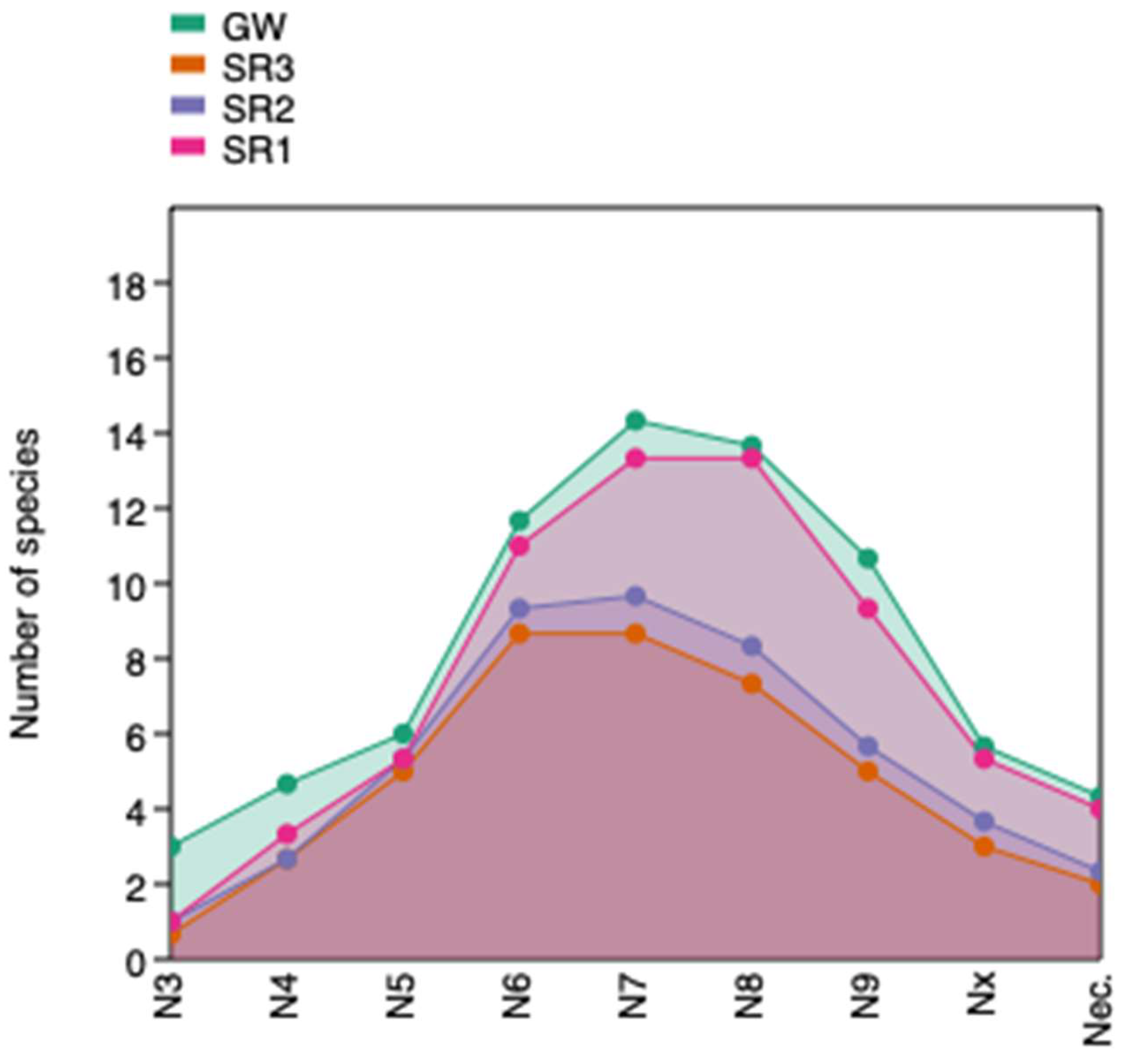
| Number of Species | N × 3 | N4 | N5 | N6 | N7 | N8 | N9 | Nx * | Nec. * |
|---|---|---|---|---|---|---|---|---|---|
| 95 | 3 | 3 | 12 | 8 | 27 | 19 | 9 | 10 | 2 |
| GW | 3 | 3 | 8 | 7 | 20 | 16 | 5 | 11 | 1 |
| SR3 | 0 | 2 | 6 | 7 | 13 | 6 | 3 | 6 | 0 |
| SR2 | 0 | 3 | 5 | 8 | 15 | 6 | 4 | 7 | 0 |
| SR1 | 0 | 3 | 7 | 6 | 20 | 14 | 6 | 8 | 2 |
| SR1 | SR2 | SR3 | GW | |
|---|---|---|---|---|
| SR1 | 0 | 10.296 | 11.533 | 5.099 |
| SR2 | 10.296 | 0 | 3.000 | 12.728 |
| SR3 | 11.533 | 3.000 | 0 | 13.892 |
| GW | 5.099 | 12.727 | 13.892 | 0 |
| Sample Point | SR1 | SR2 | SR3 | GW | |
|---|---|---|---|---|---|
| HQscore | |||||
| As | children | 0.780000 | 1.04000 * | 0.980000 | 0.440000 |
| adults | 0.185714 | 0.247619 | 0.233333 | 0.104762 | |
| Cu | children | 0.008130 | 0.010230 | 0.009660 | 0.015660 |
| adults | 0.001936 | 0.002436 | 0.002300 | 0.003729 | |
| Fe | children | 0.016560 | 0.012660 | 0.015450 | 0.017760 |
| adults | 0.003943 | 0.003014 | 0.003679 | 0.004229 | |
| Ni | children | 0.005280 | 0.006420 | 0.007500 | 0.008220 |
| adults | 0.001257 | 0.001529 | 0.001786 | 0.001957 | |
| Pb | children | 0.011100 | 0.013700 | 0.015500 | 0.018400 |
| adults | 0.002643 | 0.003262 | 0.003690 | 0.004381 | |
| Sr | children | 0.003900 | 0.004640 | 0.005500 | 0.006220 |
| adults | 0.000929 | 0.001105 | 0.001310 | 0.001481 | |
| Zn | children | 0.004456 | 0.005720 | 0.005400 | 0.013880 |
| adults | 0.001061 | 0.001362 | 0.001286 | 0.003305 | |
| Mn | children | 0.006609 | 0.006137 | 0.006026 | 0.005897 |
| adults | 0.001573 | 0.001461 | 0.001435 | 0.001404 | |
| HIscore | children | 0.83603 | 1.09951 | 1.04504 | 0.52604 |
| adults | 0.19906 | 0.26179 | 0.24882 | 0.12525 |
Disclaimer/Publisher’s Note: The statements, opinions and data contained in all publications are solely those of the individual author(s) and contributor(s) and not of MDPI and/or the editor(s). MDPI and/or the editor(s) disclaim responsibility for any injury to people or property resulting from any ideas, methods, instructions or products referred to in the content. |
© 2025 by the authors. Licensee MDPI, Basel, Switzerland. This article is an open access article distributed under the terms and conditions of the Creative Commons Attribution (CC BY) license (https://creativecommons.org/licenses/by/4.0/).
Share and Cite
Nasca, O.; Dippong, T.; Resz, M.-A.; Marian, M. Interdisciplinary Evaluation of the Săpânța River and Groundwater Quality: Linking Hydrological Data and Vegetative Bioindicators. Water 2025, 17, 1975. https://doi.org/10.3390/w17131975
Nasca O, Dippong T, Resz M-A, Marian M. Interdisciplinary Evaluation of the Săpânța River and Groundwater Quality: Linking Hydrological Data and Vegetative Bioindicators. Water. 2025; 17(13):1975. https://doi.org/10.3390/w17131975
Chicago/Turabian StyleNasca, Ovidiu, Thomas Dippong, Maria-Alexandra Resz, and Monica Marian. 2025. "Interdisciplinary Evaluation of the Săpânța River and Groundwater Quality: Linking Hydrological Data and Vegetative Bioindicators" Water 17, no. 13: 1975. https://doi.org/10.3390/w17131975
APA StyleNasca, O., Dippong, T., Resz, M.-A., & Marian, M. (2025). Interdisciplinary Evaluation of the Săpânța River and Groundwater Quality: Linking Hydrological Data and Vegetative Bioindicators. Water, 17(13), 1975. https://doi.org/10.3390/w17131975