Abstract
The conventional practice in the design of storm drainage systems is based on statistically stationary load and resistance conditions that remain invariant over time. However, uncertainties in the variables affect the design accuracy and the satisfactory performance of these hydrosystems during their operation and service. To overcome this limitation, a design methodology for a storm drainage channel was proposed using a probabilistic framework that incorporates uncertainty analysis of random variables and estimates the system’s probability of failure in terms of design depth and maximum allowable velocity. This methodology employs the Monte Carlo simulation technique and offers an alternative design and analysis approach to strengthen the conventional sizing method for drainage channels in urban watersheds. Based on uncertainty criteria associated with hydraulic design, operation, and prospective changes in the watershed and the channel, appropriate dimensions were estimated regarding design depth and freeboard. The results of this study demonstrate that the annual probability of failure of a channel, when considering uncertainty, is significantly higher than the yearly exceedance probability associated with the hydrological design return period event. Therefore, the proposed methodology is appropriate for estimating the system’s capacity and potential failure risk. This methodology may also be applied to sizing other stormwater drainage structures.
1. Introduction
Stormwater drainage systems are fundamental for urban infrastructure. However, in many cities, their condition deteriorates over time, compromising their optimal performance and proper service. A stormwater drainage system is exposed to random physical interactions that do not remain constant over time, making it susceptible to natural or anthropogenic external stresses that may cause failures in any of the system’s components throughout its service life. For example, the convergence of urban expansion, deteriorating infrastructure, and a changing climate will escalate the risks of urban flooding in the coming decades [1].
A stormwater drainage system’s design traditionally uses deterministic parameters, but they exhibit probabilistic behavior due to uncertainty, and natural and/or inherent randomness [2]. This affects the system’s response and performance, which is conventionally designed under stationary conditions. The performance of an urban water system depends on the load and the system’s response characteristics. The latter may be affected by the interactions between the various subsystems and may change over time or even during an event [3].
The return period is the design criterion commonly used for sizing stormwater drainage systems; therefore, the risk of system failure is considered equal to the exceedance probability of design rainfall. According to Melchers, R. E., & Beck, A. T. [4], this represents a theoretical disadvantage as it only accounts for the average time between events without considering how they interact with the system’s resistance.
In engineering, the potential failure of a system occurs due to the combination of the inherent randomness of external loads and various uncertainties involved in the process [5]. The primary sources of uncertainty include measurement errors, representation of unpredictable or stochastic events, misconceptions about the studied system, and operational uncertainties related to construction, manufacturing, deterioration, maintenance, and human activities [6,7]. For example, two significant sources of uncertainty in channel design are the inaccurate estimation of the design discharge and its daily and seasonal variation, or the imprecise selection of Manning’s roughness coefficient [2,8,9]. Therefore, to ensure the safety of channels, it is necessary to develop designs based on reliability and uncertainty analysis instead of deterministic designs, which may lead to channel failure by ignoring the uncertainty of variables.
The proper functioning of a stormwater drainage system depends primarily on the criteria adopted during the system’s design and the conditions during its operation. Therefore, the correct identification of loads (external forces) and resistances (capacity or strength) is the most critical factor in the design and analysis of hydrosystems [10]. Although it is impossible to accurately estimate the hydrological loads to which an infrastructure will be subjected, it is possible to calculate different levels of uncertainty for various system components, which helps minimize the probability of failure [5].
In Colombia, stormwater drainage systems are designed under time-invariant stationary conditions, meaning the uncertainty of variables in the models is not considered. However, the statistical characteristics of load or resistance change over time due to the progressive urbanization changes in a watershed, which violates the stationarity assumption of the design [5]. Urbanization changes natural landscapes by adding impervious surface area, which increases the amount of precipitation turning into surface runoff [11]. As a result, watersheds change land use and cover, and a transformation in their response to rainfall events, leading to increases in peak discharge, as well as in the flow volume and velocity within the drainage network. This makes urban dwellers more prone to flood damage.
Flooding and overflows in urban areas are also the result of changes in the statistical characteristics of rainfall. Therefore, estimating extreme precipitation from a set of observed data involves various sources of uncertainty [12]. This suggests that the design of rain associated with a given return period is a parameter subject to uncertainty. In Colombia, the return period is used as a design criterion to determine the system’s total capacity.
Other sources of uncertainty that may lead to system failure are related to analysis, construction, and operational procedures. For example, the stability of a drainage channel can be affected by construction defects or sedimentation [13] or by aging, which increases the roughness of materials over time, introducing uncertainty into the flow characteristics used in the design.
Given the above, it is essential to evaluate the probability that a stormwater drainage system will meet the performance requirements defined during its design. This evaluation must focus on uncertainty and reliability analysis to estimate the probability of failure by considering the variation in model variables and ensuring that the infrastructure fulfills its intended function throughout its service life.
2. Methodology
This study presents the design of stormwater drainage channels incorporating uncertainty analysis of hydrological and hydraulic variables, along with reliability models defined for both stationary and non-stationary conditions driven by changes in land use within the watershed and hydraulic conditions of the channels (Figure 1).
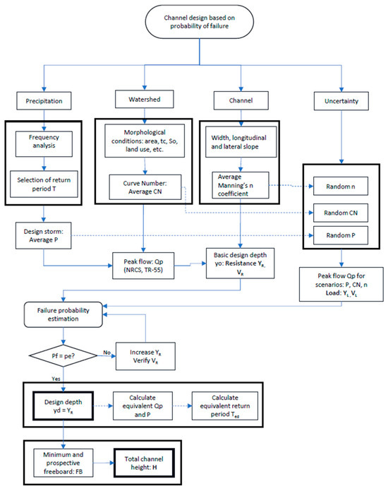
Figure 1.
Proposed design of stormwater drainage channels.
The methodology employs a Monte Carlo simulation to determine the probability of failure of the system, accounting for the uncertainty of the variables involved in flow depth. An urban watershed in Barranquilla was used as a case study. Using this methodology, the dimensions of the channel’s geometric section were estimated based on the projected potential uncertainty in the channel and watershed due to deterioration and land use changes.
To develop the proposed methodology, the following five stages were completed:
- Identification and characterization of uncertain variables: This phase involves identifying and selecting uncertain hydrological and hydraulic variables related to load and resistance that influence the design, analysis, and operation of storm drainage systems, potentially affecting system reliability. The selection of variables depends on the extent to which their uncertainty is relevant to the design, considering watershed and channel conditions, field measurement techniques or technologies, model calibration, construction processes, and other factors. The dominant uncertain variables are represented using statistical properties that describe their random behavior, according to the probability density function (PDF) assigned to each variable.
- Definition of reliability criteria and failure risk: To conduct an uncertainty analysis of storm drainage systems, the performance function is defined to quantify the system’s probability of failure. The performance function considers load and resistance as follows: and , respectively, where , are stochastic variables. The system failure risk, or probability of failure, is defined as the probability P that the load L exceeds the resistance R. In the analysis of drainage channels, the variable of interest considers the load L as the depth and velocity of the flow associated with a given discharge and the hydraulic conditions of the channel, while the resistance R corresponds to the design depth (excluding freeboard) and the maximum allowable velocity within the channel.
- Definition of the study area: This section includes delineating a consolidated and instrumented urban watershed and the hydrological characterization of its drainage area. It consists of geometrically dimensioning the cross-section of a drainage channel in accordance with Colombian guidelines (RAS [14]), based on the drainage area of the selected watershed.
- Construction of stationary and non-stationary synthetic scenarios and evaluation of failure criteria: Using the rainfall-runoff model, at least 50,000 synthetic load scenarios are defined through the Monte Carlo simulation technique, considering the uncertainty of the variables selected for four uncertainty scenarios, representing a total of 200,000 events. The synthetic resistance scenarios are determined for different return period events and calculated based on a frequency analysis that considers the typical soil conditions of an urban watershed. To estimate the system’s probability of failure, the resistance values are evaluated against each random load event within the performance function defined for each load uncertainty scenario.
- Sizing drainage channels based on the proposed methodology: The geometric section sizing is carried out, focusing on estimating the channel’s design depth and total height for a rectangular concrete hydraulic section. This process considers uncertainty in the hydrological–hydraulic models involved in channel design.
2.1. Uncertain Variables Defined for the Model
In the sizing of drainage channels for urban watersheds, the NRCS method (Natural Resources Conservation Service) is commonly used to estimate the peak discharge () as it allows not only to consider soil heterogeneity, infiltration, and spatially variable land use through the estimation of the curve number (CN), but also the percentage of permeable and disconnected areas, and the implementation of Sustainable Urban Drainage Systems (SUDS), among other advantages.
The general equation proposed by the NRCS [15] for calculating the surface runoff (adequate precipitation) is defined as follows:
where is the surface runoff or effective precipitation (mm), P is the total 24 h precipitation (mm), is potential maximum retention after runoff begins (mm), and represents the initial abstraction (mm).
The NRCS developed an empirical relationship to estimate based on the evaluation of the effects of land use and conservation practices on direct runoff. This relationship is expressed as follows:
To transform surface runoff into peak discharge, the NRCS TR55 model [15] is used, which defines peak discharge as follows:
where is the unit peak discharge (m3/(s·cm·km2), A is the watershed area (km2), is the surface runoff (cm) generated by a 24 h storm for a defined return period, and is the pond and swamp adjustment factor (dimensionless), which is equal to 1.0 when such areas are not considered.
In this study, the curve number (CN) and the precipitation (P) were identified as variables with a high level of uncertainty.
In the sizing of the channel’s geometric section, hydraulic variables also introduce a legitimate degree of uncertainty in estimating the channel’s hydraulic capacity or resistance, considering conditions during the construction and operation phases of the system. To calculate the channel capacity in terms of discharge, flow depth, or flow velocity, Manning’s equation was applied, given the discharge and the channel properties:
where is the discharge (m3/s), is the cross-sectional area (m2) (in this study, a rectangular channel was analyzed), is the hydraulic radius (m), is the energy slope (m/m), and n is Manning’s roughness coefficient (s/m0.33).
For the estimation of the system’s capacity, Manning’s roughness coefficient n was considered the dominant hydraulic variable with associated uncertainty in the model as its average value may vary over time due to the material and environmental conditions of a concrete-lined structure.
2.1.1. Precipitation (P)
To represent the uncertainty associated with precipitation (P), a frequency analysis of the annual maximum daily precipitation was conducted, showing a good statistical fit of a Gumbel probability distribution to the historical series associated with the study watershed with a p-value = 0.090. So, the mean precipitation corresponds to the value obtained from the Gumbel distribution for the design return period, and the random error was represented by a normal distribution in which the standard deviation was derived from the confidence interval limits of each quantile.
The cumulative density function, , of the Gumbel distribution is defined as follows:
where is the random variable representing an extreme precipitation amount, is the location parameter, and is the scale parameter.
The expected precipitation value (quantile) associated with the return period was determined using the following expression:
where and are the location and scale parameters, with values of 71.1572 and 18.3123, respectively.
The frequency analysis results for various return periods of interest, typically used in channel design, are presented in Table 1.

Table 1.
Frequency analysis results.
2.1.2. Curve Number (CN)
McCuen [16] estimated the confidence intervals of the CN from five urban watersheds based on the gamma probability distribution instead of using a minimum or maximum value on the Antecedent Moisture Condition (AMC); however, the author mentioned that any other probability distribution may be used if the CN values are consistent with the watershed. Additionally, Farran & Elfeki [17] estimated the confidence interval of CN by using both the beta and gamma probability distribution, obtaining similar results. Therefore, the beta probability distribution was used for representing the behavior of the curve number (CN) in this case study, given it is possible to estimate a constant standard deviation for all the CN cases.
The beta distribution is bounded between 0 and 1; therefore, the mean value of the distribution was set as , where the CN value is obtained from the NRCS tables according to the identified characteristics of the urban watershed. The PDF of the beta distribution is defined as follows:
for values , where is the beta function, defined for .
The confidence intervals were determined for each CN value, each with a mean and corresponding α and parameters. This study set the CN values at 75, 80, 85, 90, and 95, consistent with typical urban areas.
To estimate the parameters of the distribution, the following formulas were used:
where is the mean, given by , and is the standard deviation, with an adjusted value of 0.063.
The confidence intervals were obtained from the cumulative distribution function (CDF) using a 10% significance level for a two-tailed test, to validate the results against those reported by McCuen [16] (Figure 2), which were verified using the AMC limits.
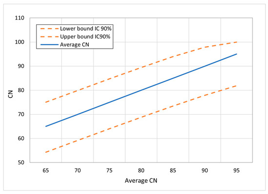
Figure 2.
Plot of confidence intervals for curve number (CN).
2.1.3. Manning’s Roughness Coefficient ()
Chin [18] defines a range of ±0.0045 on the Manning’s roughness coefficient for float finish concrete; however, this may suggest a channel has the same probability of having lower or higher Manning’s coefficient. Also, a maximum high limit roughness coefficient is set when it may actually be higher due to deterioration by environmental conditions. Therefore, to have more flexibility on the uncertainty behavior of the Manning’s coefficient, a gamma probability distribution PDF was selected to estimate the uncertainty associated with the variable . However, designers may select any other probability distribution that fit with their assumptions or available data.
For a continuous random variable that follows a gamma distribution with parameters and , the PDF is expressed as follows:
for , where is the gamma function.
This study analyzed uncertainty for mean values of 0.015, 0.017, 0.019, and 0.021 s/m0.33. To generate random values of Manning’s roughness coefficient associated with each mean value, a gamma distribution PDF with parameters and was used, with a fixed minimum threshold value of 0.011 s/m0.33.
Figure 3 shows that Manning’s roughness coefficient can physically range between 0.011 and values greater than 0.03 s/m0.33. However, the probability of high coefficients is lower when the mean coefficient is 0.015 s/m0.33, and increases as the mean coefficient rises to 0.021 s/m0.33.
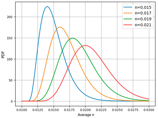
Figure 3.
Proposed PDF with gamma distribution for n = 0.015, 0.017, 0.019, and 0.021 s/m0.33.
2.2. Uncertainty Criteria
Two failure modes were considered for drainage channels: one associated with flow depth and the other with channel erosion, analyzed based on flow velocity.
2.2.1. Failure Mode 1
The flow depth exceeds the design depth of the channel (excluding freeboard), i.e., .
The performance function for Failure Mode 1 is defined as the difference between the channel resistance and the load . For the case study, a sufficiently long channel was assumed, so the load and the resistance were calculated using Manning’s equation.
2.2.2. Failure Mode 2
The flow velocity exceeds the maximum allowable velocity due to erosion, i.e., .
The performance function for Failure Mode 2 is defined as the difference between the maximum permissible velocity due to erosion , determined according to the channel material, and the flow velocity , which is calculated using Manning’s equation under the assumption of a sufficiently long channel.
The probability of failure was calculated using the Monte Carlo simulation technique, defined as follows:
where is the number of simulations and is the indicator function evaluated on the performance function . If , then ; otherwise,
2.3. Study Area
The Torcoroma Watershed is a fully developed urban watershed located in the northern part of Barranquilla, Colombia. It has an area of 142 hectares, and the main channel is approximately 1.6 Km long (Figure 4). The land use is predominantly residential and commercial. The watershed has an average slope = 3%, which results in supercritical flow conditions on the streets during rainfall events [19].
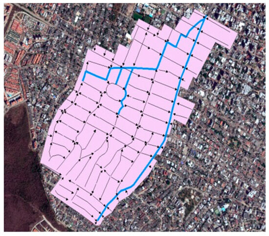
Figure 4.
Torcoroma watershed and street flow directions.
Available field data on water depth and velocity were collected between 23 August and 7 September 2014. Table 2 shows each recorded event’s total precipitation and peak discharge records (23 August, 28 August, and 7 September 2014).
Table 2.
Field data measured between 23 August and 7 September 2014.
2.3.1. Calibration of the Torcoroma Watershed: Rainfall-Runoff Model
Surface runoff was calculated from the field data by calibrating the CN parameter on the TR-55 method [15]. A CN = 96 achieved the best fit between the observed and simulated data (Table 3). The model calibration was assessed using the coefficient of determination R2, a parameter commonly used to calibrate and validate urban watersheds. The calibration results determined R2 = 0.94, corresponding to a good fit considering the observed flows.
Table 3.
Rainfall-runoff model calibration results for the Torcoroma watershed.
The watershed’s time of concentration was estimated at Tc = 0.23 h, considering a Manning coefficient of 0.015 s/m0.33 for the watershed surface and an average slope = 3%.
2.3.2. Conventional Sizing of Drainage Channels
According to the Colombian technical guidelines (RAS [14]), the design return period for a drainage area of 142 hectares is 50 years. A rectangular concrete drainage channel was designed with a width b = 6.0 m and a longitudinal slope (Figure 5).
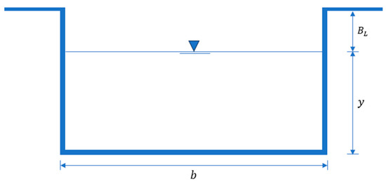
Figure 5.
Hydraulic cross-section of a rectangular drainage channel.
To assess the channel’s behavior under changes in land use and cover, surface runoff was estimated for three design scenarios with CN values of 85, 90, and 95. The watershed calibration results kept other model parameters constant.
Table 4 shows the results of the rainfall-runoff model and the channel resistance values in terms of flow depth and permissible velocity for each design CN. The maximum allowable velocity was selected assuming a simple reinforced concrete channel with a regular finish and a strength of 12.75 MPa [20].
Table 4.
Rainfall-runoff model results for a 50-year return period event.
3. Results
3.1. Risk Scenario Assessment for Drainage Channels
Considering several land cover conditions, synthetic resistance scenarios were determined for different design return period events. Each selected return period (2, 5, 10, 25, 50, and 100 years) was evaluated for CN values of 75, 80, 85, 90, and 95, typical for urban areas. The resistance in terms of flow depth was determined using Manning’s equation, assuming a roughness coefficient n = 0.015 m/s0.33 considered as a typical design value.
To estimate the probability of failure based on the performance functions and , 50,000 synthetic load scenarios were generated using the Monte Carlo simulation for four uncertainty scenarios where each event corresponded to a combination of the random variables of P, CN, and n. This approach aimed to assess the channel’s behavior under the influence of each random variable incorporated.
Four main scenarios were configured for evaluation based on the number of variables for which uncertainty is considered.
- -
- Scenario I (SSS): No uncertainty was considered in the variables , CN, and .
- -
- Scenario II (SSA): Uncertainty was considered only in the variable .
- -
- Scenario III (SAA): Uncertainty was considered in the variables CN and . The variable was assumed to be deterministic, taking the mean value of the quantile associated with the return period of the event.
- -
- Scenario IV (AAA): Uncertainty was considered in all variables , CN, and .
The Monte Carlo simulation was applied to each variable depending on the selected scenario. Precipitation magnitudes were randomly generated with the Gumbel probability distribution and then randomly dispersed with a normal probability distribution based on the confidence interval at each synthetic precipitation magnitude. Then, the CN was randomly generated based on the selected mean value and dispersed with the beta probability distribution. Finally, the Manning’s roughness coefficient (n) was generated based on the mean value (0.015 s/m0.33) and dispersed with the gamma distribution. Table 5 shows the characteristics of each variable described above.
Table 5.
Summary of random variable characteristics for scenarios.
3.1.1. Evaluation of Failure Mode 1
Figure 6 shows the probability of failure graphs as a function of the design return period for each scenario evaluated. The results indicate that in Scenario I (SSS), where no uncertainty was considered, the probability of failure closely follows the exceedance probability across different return periods (~). However, in Scenarios II, III, and IV, where uncertainty was introduced into one or more variables, increasingly deviates from as the return period increases ( > ). This suggests that neglecting uncertainty may lead to underestimating the probability of failure, particularly for extreme events. This was verified by performing a one-sample Student’s t-test for each case.
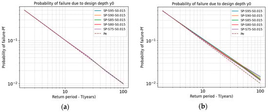
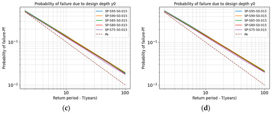
Figure 6.
Probability of failure plots—Failure Mode 1: (a) Scenario I(SSS); (b) Scenario II (SSA); (c) Scenario III(SAA); (d) Scenario IV(AAA).
In the test, the following hypotheses were formulated:
- -
- Null hypothesis: .
- -
- Alternative hypothesis: .
where is the sample mean, which corresponds to the average probability of failure for all CN values for each return period, and the hypothetical mean corresponds to the exceedance probability associated with the rainfall return period.
The results of the test (Table 6) confirm that when the uncertainty of these variables is incorporated into the models, the calculated is statistically greater than .
Table 6.
Hypothesis test results.
For example, for a two-year return period, although there is a statistically significant difference between the probability of failure and the annual exceedance probability, the difference is relatively small, around 5%. For a five-year return period, this difference increases to approximately 25%. However, for higher return periods, specifically 50 and 100 years, the probability of failure is 89% and 110% higher than the annual exceedance probability, respectively.
This means that assuming the risk of failure of a drainage channel to be equal to the annual exceedance probability leads to an underestimation of the channel dimensions making it highly likely that the structure will fail more frequently, especially for extreme events with more extended return periods.
3.1.2. Evaluation of Failure Mode 2
For Failure Mode 2, is lower than for all four scenarios. This indicates that the channel’s resistance effectively ensures that the probability of failure due to erosion is lower than the expected annual exceedance probability and, consequently, lower than the overall probability of failure (Figure 7).
Figure 7.
Probability of failure plots—Failure Mode 2: (a) Scenario I (SSS); (b) Scenario II (SSA); (c) Scenario III (SAA); (d) Scenario IV (AAA).
3.1.3. Risk of Failure Assessment for the Calibrated Watershed
The probability of failure was estimated considering the three proposed design conditions for the case study. For these conditions, a 50-year return period was selected, meaning that the expected probability of failure should be 2%, corresponding to the annual exceedance probability. The results are shown in Figure 8.
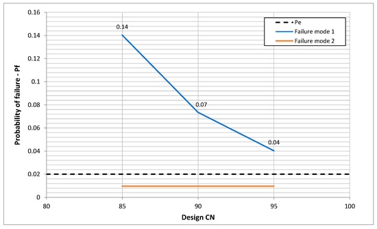
Figure 8.
Probability of failure () plot for the current conditions of the case study for the three proposed designs.
The probability of failure in Failure Mode 1 is greater than 2% for the three proposed designs. For the design CN of 85, the actual probability of failure is 14%, and for the designs of 90 and 95, the probability of failure is 7% and 4%, respectively. Given the watershed conditions, a canal designed under any of the three scenarios has a higher annual probability of failure than expected based on the exceedance probability.
For Failure Mode 2, the probability of failure due to velocity remains below the exceedance probability with a constant value of 0.97% for all the designs. This occurs because, although the system’s load increases, it does not frequently exceed the channel’s resistance velocity. However, if changes in the watershed are significant, the probability of failure may increase since the system’s load flow is higher. Nevertheless, under the conditions in which the case study was evaluated, the probability of failure was never greater than the probability of exceedance because the maximum velocity was sufficiently high to withstand the load generated by the increase in peak discharge. On the other hand, if an increase in channel roughness was considered, although the flow depth would be greater, the roughness would reduce the velocity within the channel; therefore, the probability of failure due to velocity would decrease. Failure due to erosion largely depends on the maximum allowable velocity associated with the material selected for the channel and the watershed conditions.
Figure 9 shows the PDFs of the and loads relative to the design depth for each NC evaluated, 85, 90, and 95 (strength). Each figure shows the probability of failure represented in the area with values of or .
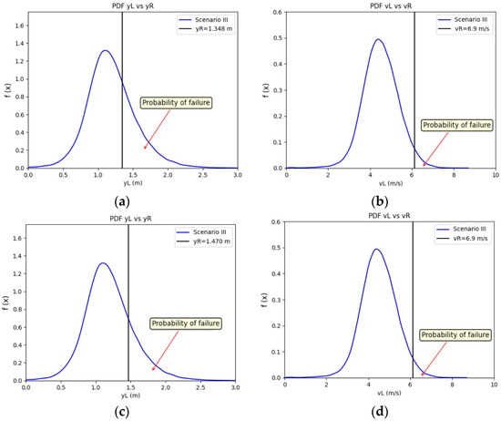
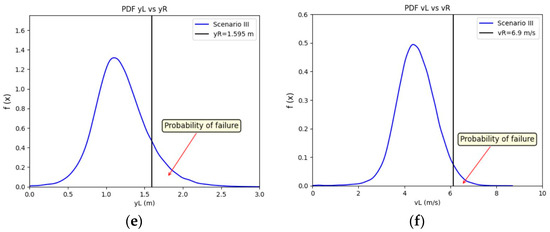
Figure 9.
Probability density function (PDF) of the load and related to the resistance and R for a design with the following: (a,b) CN = 85 and n = 0.015 s/m0.33; (c,d) CN = 90 and n = 0.015 s/m0.33; (e,f) CN = 95 and n = 0.015 s/m0.33.
3.1.4. Equivalent Return Period
The methodology presented aims to ensure the annual design exceedance probability equals the system’s yearly probability of failure. However, it was found that for Failure Mode 1, in Scenario IV, where the uncertainty of all selected random variables is included, the calculated probability of failure is greater than the annual exceedance probability for a basic design depth estimated from conventional design. This means that assuming a channel’s failure risk is equal to the yearly exceedance probability would lead to an underestimation of channel dimensions, making failure more likely. Therefore, it is necessary to determine the values of that satisfy the criterion when including the uncertainties of all random variables that define the load in hydrological–hydraulic models. This requires designing with a higher return period so that the channel’s capacity can withstand the loads it is subjected to regarding flow depth.
For this, the return period of the new load Qp corresponding to the value of that ensures the criterion was analyzed. According to the results, the mean of the equivalent design return periods () is greater than the rainfall return period (T). In general, after evaluating different scenarios of T (between 2 and 100 years) and CN (between 75 and 95), it was found that the relationship between and T is not linear but slightly curved as CN and T increase. Therefore, an equation to calculate the equivalent return period as a function of the design return period of interest was proposed (Figure 10). The equations were estimated for each CN and are expressed as follows:
where is the rainfall return period and is a coefficient based on the uncertainty results from Scenario IV (Table 7).
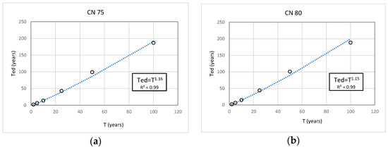
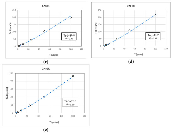
Figure 10.
Regression fits for the equivalent return period for the following: (a) CN = 75, (b) CN = 80, (c) CN = 85, (d) CN = 90, and (e) CN = 95.
Table 7.
Equivalent return periods.
3.2. Estimation of Final Design Depth
For the case study, a hypothetical scenario was proposed, the conventional drainage channel design was established for CN = 85, a roughness coefficient of 0.015 s/m0.33, and designed depth of , identified as 85 in Table 8 with a probability of failure of 0.0339, greater than the theoretical exceedance probability of 0.02 (separated by dash lines in Table 8). Possible channel deterioration and changes in the watershed’s CN were evaluated to estimate the actual probability of failure under these prospective conditions for a 50-year return period event (Table 8), considering Scenario IV.
Table 8.
Probability of failure for conventional design with CN = 85 and n = 0.015 s/m0.33.
Table 8 shows the actual probability of failure estimated for the conventional design with a considering several combinations of Manning’s coefficients and CN (n/CN). The combination n/CN 0.015/75, 0.015/80, and 0.017/75 has a probability of failure lower than 2% (for a 0-year return period). However, all the other combinations have a probability of failure greater than 2%, including the conventional design condition of n/CN = 0.015/85 with a . As the Manning coefficient and the CN increase, the probability of failure may increase up to 40% if the Manning coefficient increases to 0.021 s/m0.33. The CN increases to 95, corresponding to a case where the channel deteriorates considerably, and the land use and stormwater management practices are not adequately implemented over time.
To ensure the required design, the probability-based design depth was estimated, which is equal to the basic design depth plus a depth increment due to uncertainty (Figure 11).
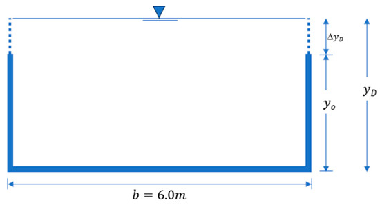
Figure 11.
Hydraulic cross-section for probability of failure-based sizing.
In other words, is also equivalent to the that fulfills the criterion of . Then, the depth that satisfies this criterion is . Table 9 shows the updated probability of failure estimation but with a instead of the conventional , ensuring the criterion
Table 9.
Probability of failure for probability of failure-based design with CN = 85 and n = 0.015 s/m0.33.
However, if the channel or the watershed roughness conditions change by increasing either the Manning coefficient or the CN, the probability of failure would again exceed 2%; for example, if the mean value of n increases from 0.015 s/m0.33 to 0.021 s/m0.33, and the CN increases to 95, the probability of failure would be 29.8%.
Increases in the return period do not necessarily represent a drastic increment in the design depth. For a 2-year return period, the equivalent return period is approximately 2.2 years; for a 25-year return period, the equivalent return period is approximately 42 years; and for a 100-year return period, it is approximately 210 years. In the case study, for a 50-year design period, the equivalent return period was approximately 94 years, or 88% greater; however, the depth increased only by 9%. This increment in depth guarantees a known probability of failure consistent with the expected annual design exceedance probability.
3.2.1. Estimation of Freeboard
The methodology proposes a freeboard criterion that modifies Chin’s recommendations [18]. Still, it incorporates the probability-based design depth and additional heights at the designer’s discretion to account for channel deterioration, land use changes in the watershed, non-stationary rainfall conditions, and other critical hydraulic factors beyond waves, winds, splashing, and turbulence, as the freeboard usually accounts for.
3.2.2. Prospective Water Depth and Estimation of an Initial Freeboard
The initial freeboard is an additional height associated with uncertainty for prospective scenarios of channel deterioration and increases in CN that the designer may consider. It is expressed as follows:
where corresponds to the prospective water depth estimated with the same probability-based methodology used for estimating , but considering the uncertainty due to the prospective channel deterioration and increases in CN for the future defined by the designer.
Continuing with the case study, the probability-based design depth for CN = 85 and n = 0.015 s/m0.33 is .
Then, assuming hypothetical future scenarios of increments of CN to 90 and 95 and increments of Manning’s coefficient in the channel to 0.017, 0.019, and 0.021 s/m0.33, the water depth may increase from to maintaining the criterion of . Table 10 shows the results of required for those scenarios.
Table 10.
Required resistance (m) for a 2% probability of failure for the scenarios for a design with CN = 85 and n = 0.015 s/m0.33.
The magnitudes of do not correspond to the channel design depths, but rather to the total channel height that includes the design depth and an initial freeboard that accounts for uncertainty due to deterioration and increased CN. Based on these magnitudes, the designer must estimate a total freeboard to obtain the final channel height .
Table 11 shows the values of the initial freeboard .
Table 11.
Initial freeboard (m) required for prospective roughness and CN scenarios with a 2% probability of failure for a design with CN = 85 and n = 0.015 s/m0.33.
After estimating the initial freeboard , it is necessary to include additional heights based on the following criteria:
When the design depth is less than 0.30 m, the freeboard would be as follows:
When the design depth is greater than 0.30 m and the flow velocity is less than 1.72 m/s, in order to account for waves, wind, splashing, and turbulence, the freeboard would be as follows:
Finally, when the design depth is greater than 0.30 m and the flow velocity exceeds 1.72 m/s, it is necessary to include a minimum of 0.15 m plus the initial freeboard and the velocity head associated with prospective water depth (). For this condition, the freeboard is expressed as follows:
For this case study, the flow depth is greater than 0.30 m, and the flow velocity exceeds 1.72 m/s; therefore, the freeboard FB is determined using Equation (18). This criterion is more sensitive to increases in CN than to increases in channel roughness. Consequently, the worst prospective condition should be evaluated at the designer’s discretion to define an appropriate freeboard.
According to the results in Table 12, if the watershed conditions are projected to increase CN to 95 while maintaining n = 0.015 s/m0.33, the design freeboard should be 2.43 m. However, if the Manning coefficient increases to n = 0.021 s/m0.33 for CN = 95, the estimated freeboard is 2.14 m. The selected scenarios should be evaluated at the designer’s discretion.
Table 12.
Freeboard and total channel height estimated with the probability-based design methodology for CN = 85, and n = 0.015 s/m0.33.
The probability-based design depth is 8.6% greater than the conventional design depth , and the estimated freeboard using different criteria represents a safety factor between 1.7 and 2.7, with an average of 2.1. This considers the flow supercritical, and the design discharge is relatively high.
The probability of failure-based design increases the total channel depth by 7.6% compared to the conventional design for CN = 85 and n = 0.015 s/m0.33, when prospective conditions of channel deterioration and increases in CN over time are not considered. However, under a prospective condition of channel deterioration and an increase to CN = 95, the probability of failure-based design defines a channel with a total height 23.5% greater than the total depth of the conventional design, since the traditional freeboard does not account for prospective uncertainty scenarios (Table 13).
Table 13.
Comparison of channel dimensions with conventional design and probability of failure-based design.
A larger channel dimension entails higher construction costs, an essential factor to consider when developing a design. However, all necessary considerations must be made to ensure the construction of safe, adequate, and functional channels capable of withstanding the loads for which they were designed, taking into account the random behavior of the variables involved in the models, especially when the evidence has proved that the deterioration of the channel, land use changes, and potential non-stationary rainfall scenario are expected during the channel lifetime.
4. Discussion
The results of this research demonstrate that there is a significant difference between the annual probability of failure and the annual exceedance probability , especially for higher return periods when the uncertainty of random variables is not considered in channel design. This difference is marginal at a 95% confidence level; however, for return periods of 5, 50, and 100 years, the difference becomes more pronounced, with increases of 25%, 89%, and 110%, respectively. This indicates that using as the sole design criterion underestimates the required channel capacity, increasing the probability of system failure.
To satisfy the criterion , it is recommended to design using a higher return period. This adjustment leads to increases in design depth that are not disproportionate—for a 50-year return period, only a 9% increase in depth is needed—while significantly reducing the associated risk.
Among the evaluated failure modes, Mode 1 (depth) is more sensitive to uncertainty analysis than Mode 2 (velocity/erosion). In the case study, the maximum velocity was sufficient to resist the load; however, future changes in the watershed could alter this condition.
Designing without accounting for uncertainty systematically underestimates channel resistance, supporting the need to incorporate reliability and uncertainty models into design standards such as RAS [14]. Integrating reliability analysis tools can help mitigate flood risks and promote infrastructure adapted to demographic and climatic challenges, aligning with current approaches in sustainable urban planning.
5. Conclusions
A methodology for designing drainage channels based on the probability of failure was presented. This methodology allows incorporating the inherent uncertainty of hydrological and hydraulic variables in the analysis, which enables a more accurate estimation of the system’s probability of failure and, therefore, the proper sizing of the geometric sections of any channel of a stormwater drainage system.
With this methodology, it is possible to evaluate the channel’s behavior by analyzing the interaction between load and resistance, according to prospective conditions that the designer may consider in terms of probability at their discretion during the design stage. This is not possible with deterministic designs, as they do not allow for the evaluation of the channel’s response to the specific conditions of the design.
The proposed methodology required the Monte Carlo simulation to determine the system’s probability of failure, which was evaluated in terms of design flow depth and maximum allowable velocity, considering the uncertainty of the variables , CN, and . The research results demonstrated that when uncertainty is not considered in the design process, the channel’s capacity is underestimated, making it highly likely to fail under rainfall events smaller than the expected design return period. However, this disadvantage is overcome by sizing the same system based on the probability of failure and its equivalent return period to ensure the channel’s probability of failure equals the exceedance probability associated with the design return period.
A freeboard equation was proposed based on the probability of failure criterion to estimate the total height H. In this equation, the freeboard is expressed in terms of hydraulic conditions caused by wind-generated waves, splashing, and agitation, but also includes a height component associated with uncertainty due to prospective changes in the watershed and operational conditions of the channel.
Implementing this methodology has many advantages, as it enables the designer to anticipate possible future channel behaviors and, therefore, make informed decisions during the design stage to ensure the proper functioning of the structure.
Author Contributions
Conceptualization, S.A.-P. and H.A.-R.; methodology, S.A.-P., H.A.-R., O.E.C.-H., M.P.-S. and A.H.S.-C.; formal analysis, S.A.-P. and H.A.-R.; writing—original draft preparation, S.A.-P. and H.A.-R.; writing—review and editing, O.E.C.-H., M.P.-S. and A.H.S.-C. All authors have read and agreed to the published version of the manuscript.
Funding
This research received no external funding.
Data Availability Statement
Databases are available in this article.
Conflicts of Interest
Stefany Anaya-Pallares was employed by the company HYCEN SAS. The remaining authors declare that the research was conducted in the absence of any commercial or financial relationships that could be construed as a potential conflict of interest.
References
- McPhillips, L.E.; Boving, T.B.; McAndrew, A.; Shuster, W.D.; Nowosad, J.; Walsh, M. Modeling the Impact of Future Rainfall Changes on the Effectiveness of Urban Stormwater Control Measures. Sci. Rep. 2024, 14, 5289. [Google Scholar] [CrossRef]
- Gouri, R.L.; Srinivas, V.V. Reliability Assessment of a Storm Water Drain Network. Aquat. Procedia 2015, 4, 772–779. [Google Scholar] [CrossRef]
- Meijer, D.; Korving, H.; Langeveld, J.; Clemens-Meyer, F. A method to identify the weakest link in urban drainage systems. Water Sci. Technol. 2023, 87, 1273–1293. [Google Scholar] [CrossRef] [PubMed]
- Melchers, R.E.; Beck, A.T. Structural Reliability Analysis and Prediction, 3rd ed.; John Wiley & Sons: Hoboken, NJ, USA, 2017. [Google Scholar]
- Tung, Y.-K.; Yen, B.-C.; Melching, C.S. Hydrosystems Engineering Reliability Assessment and Risk Analysis; McGraw-Hill: New York, NY, USA, 2006. [Google Scholar] [CrossRef]
- Kottegoda, N.T. Stochastic Water Resources Technology; John Wiley & Sons: New York, NY, USA, 1980. [Google Scholar]
- Tung, Y.K. Uncertainty and reliability analysis in water resources engineering. J. Contemp. Water Res. Educ. 1999, 103, 4. [Google Scholar]
- Hosseini, S.M.; Mahjouri, N. Sensitivity and fuzzy uncertainty analyses in determining SCS-CN parameters from rainfall–runoff data. Hydrol. Sci. J. 2018, 63, 457–473. [Google Scholar] [CrossRef]
- Thorndahl, S.; Willems, P. Probabilistic modelling of overflow, surcharge and flooding in urban drainage using the first-order reliability method and parameterisation of local rain series. Water Res. 2008, 42, 455–466. [Google Scholar] [CrossRef] [PubMed]
- Gheorghe, A. Topics in Safety, Risk, Reliability and Quality; Springer: Dordrecht, The Netherlands, 2013; Volume 22. [Google Scholar]
- Almadani, A.; Parajuli, P.B.; Moriasi, D.N. Effectiveness of Design and Implementation Alternatives for Stormwater Control Measures Modeled at the Watershed Scale. Hydrology 2023, 10, 49. [Google Scholar] [CrossRef] [PubMed]
- Birk, J.; Thorndahl, S.; Schaarup-Jensen, K.; Jensen, J.B. Probabilistic modelling of combined sewer overflow using the First Order Reliability Method. Water Sci. Technol. 2008, 57, 1269–1275. [Google Scholar] [CrossRef]
- Adarsh, S.; Reddy, M.J. Reliability analysis of composite channels using first order approximation and Monte Carlo simulations. Stoch. Environ. Res. Risk Assess. 2013, 27, 477–487. [Google Scholar] [CrossRef]
- Ministerio de Vivienda, Ciudad y Territorio (Minvivienda). Resolución 0330 de 2017. Reglamento Técnico del Sector de Agua Potable y Saneamiento Básico-RAS. Available online: https://www.minvivienda.gov.co/viceministerio-de-agua-y-saneamiento-basico-reglamento-tecnico-sector-reglamento-tecnico-del-sector-de-agua-potable-y-saneamiento-basico-ras (accessed on 23 June 2025).
- USDA (United States Department of Agriculture). Estimation of Direct Runoff from Storm Rainfall, Chapter 10. In National Engineering Handbook; Mockus, V., Hjelmfelt, A.T., Eds.; Natural Resources Conservation Service: Washington, DC, USA, 2004. [Google Scholar]
- McCuen, R.H. Approach to Confidence Interval Estimation for Curve Numbers. J. Hydrol. Eng. 2002, 7, 143. [Google Scholar] [CrossRef]
- Farran, M.M.; Elfeki, A.M. Statistical Analysis of NRCS Curve Number (NRCS-CN) in Arid Basins Based on Historical Data. Arab. J. Geosci. 2020, 13, 1. [Google Scholar] [CrossRef]
- Chin, D.A. Water-Resources Engineering, 3rd ed.; Prentice Hall: Upper Saddle River, NJ, USA, 2013. [Google Scholar]
- Avila, H.; Avila, L.; Sisa, A. Dispersed Storage as Stormwater Runoff Control in Consolidated Urban Watersheds with Flash Flood Risk. J. Water Resour. Plan. Manag. 2016, 142. [Google Scholar] [CrossRef]
- Sotelo Ávila, G. Volumen 1: Fundamentos. In Hidráulica General; Limusa: Lorca, Spain, 2010; 561p. [Google Scholar]
Disclaimer/Publisher’s Note: The statements, opinions and data contained in all publications are solely those of the individual author(s) and contributor(s) and not of MDPI and/or the editor(s). MDPI and/or the editor(s) disclaim responsibility for any injury to people or property resulting from any ideas, methods, instructions or products referred to in the content. |
© 2025 by the authors. Licensee MDPI, Basel, Switzerland. This article is an open access article distributed under the terms and conditions of the Creative Commons Attribution (CC BY) license (https://creativecommons.org/licenses/by/4.0/).