Abstract
This study investigated the influence of long-term climatic phenomena on the hydroclimatic dynamics of the Grey River Basin in Chilean Patagonia. By analyzing hydroclimatological datasets from the last four decades (1980 to 2020), including precipitation, temperature, wind speed, potential evapotranspiration, and streamflow, we identified key trends and correlations with three large-scale climate indices: the Antarctic Oscillation (AAO), El Niño—Southern Oscillation (ENSO), and Pacific Decadal Oscillation (PDO). Statistical methods such as the Mann–Kendall test, Sen’s slope, PCA, and wavelet coherence were applied. The results indicate a significant upward trend in streamflow, with Sen’s slope of 0.710 m3/s/year (p-value = 0.020), particularly since 2002, while other variables showed limited or no significant trends. AAO exhibited the strongest correlations with streamflow and wind speed, while ENSO 3.4 was the most influential ENSO index, especially during the two extreme El Niño events in 1982, 1997, and 2014. PDO showed weaker relationships overall. Wavelet analysis revealed coherent periodicities at 1- and 2-year frequencies between AAO and flow (wavelet coherence = 0.44), and at 2- to 4-year intervals between ENSO and precipitation (wavelet coherence = 0.63). These findings highlight the sensitivity of the Grey River basin to climatic variability and reinforce the need for integrated water resource management in the face of ongoing climate change.
1. Introduction
The three interconnected environmental challenges of climate change, biodiversity, and pollutant emission, collectively referred as the triple planetary crisis, pose severe threats to human well-being, socioeconomic systems, and the long-term sustainability of our planet [1]. These challenges are not isolated: they interact synergistically, exacerbating each other and creating complex issues that require comprehensive and immediate attention [2,3,4]. To effectively address these pressing concerns, urgent and coordinated global action is imperative [5].
In this context, climate change stands out as the most formidable threat to human health in the 21st century [6]. The relentless increase in greenhouse gas emissions has led to a significant rise in global temperatures, disrupting weather patterns and endangering critical ecosystems such as wetlands [7]. The anticipated average global temperature rise of 1.5 °C to 2 °C above pre-industrial levels is projected to have catastrophic consequences for life on Earth [8]. Increasing water scarcity affects billions of people, leading to heightened competition for limited water resources [9]. At the same time, the rising frequency and intensity of extreme precipitation and flooding are a significant threat to communities, infrastructure, and economies [10,11]. A tenfold acceleration in the melting of Arctic ice contributes to rising sea levels and the loss of habitat for polar species [12], which may cause the near-complete disappearance of coral reefs, vital for marine biodiversity, coastal protection, and fisheries [12]. A 50% reduction in crop yields threatens global security and exacerbates hunger and malnutrition [13]. Significant declines in seafood production, plant species, and insect populations disrupt ecosystems and their services [14].
In Chile, water scarcity has escalated to alarming levels in recent years, becoming a pressing issue that affects millions of residents and the country’s agricultural productivity [15]. Since 2010, Chile has been facing a significant and sustained decline in rainfall, with reductions of up to 25% in the central region over the last few decades [16,17]. This prolonged period of diminished precipitation, often referred to as megadrought, has had profound implications for the country’s water resources [18]. The effects of this megadrought are particularly evident in the substantial decrease in the flow of critical rivers that are vital for sustaining both human populations and agricultural activities [19,20]. Major rivers, which historically provided reliable sources of water, have been affected by a drastic decrease in their flow, leading to severe water shortages [21]. This situation adversely impacts the availability of water for human consumption, leading to concerns about public health and quality of life [22,23]. Furthermore, the reduction in water supply poses significant challenges for agricultural irrigation, a cornerstone of Chile’s economy [24]. Many farmers are facing difficulties in accessing sufficient water for their crops, which not only threatens food security but also jeopardizes the livelihoods of those dependent on agriculture [25]. The economic repercussions of water scarcity extend beyond individual farms, affecting entire communities and the nation’s food production capabilities [26].
Nonetheless, Chilean Patagonia has also suffered the consequences of climate change, which have significantly impacted nivo-pluvial basins [27,28] and glacier dynamics [29]. In this tundra environment, rising temperatures cause permafrost to thaw, destabilizing the ground, releasing stored carbon dioxide and methane into the atmosphere, and accelerating global warming [30]. This thawing alters local hydrology, increasing soil moisture variability, changing river flow patterns, and affecting the availability of freshwater for both ecosystems and human needs [31]. Additionally, this zone is influenced by long-term climate variability, such as the westerly wind [32,33]. While most studies have focused on watersheds in the Northern Hemisphere, research in the Southern Hemisphere remains limited [34]. Studies in the Northern Hemisphere have not found significant relationships between a wide range of climate variables and various large-scale climate phenomena [35,36,37,38]. In addition to the above, most of the studies carried out in Patagonia focus on glacier dynamics, but not at the basin level [39,40,41], while studies that include the evaluation of various hydrological processes are scarce [42].
As Chile faces mounting water-related challenges, the urgency to address the root causes of water scarcity and to implement effective management strategies grows increasingly clear and is essential to secure a sustainable water supply for future generations [34]. In this context, the objective of this work was to analyze the hydroclimatic variables of the Grey River Basin in Chilean Patagonia, aiming to innovate in assessing how large-scale climatic phenomena affect this watershed. Unlike traditional approaches, our results not only detect correlations across different timescales but also identify specific periods of high climatic significance.
2. Materials and Methods
2.1. Study Area
The study area corresponds to the Grey River basin, up to the fluviometric station Río Grey Antes Junta Río Serrano (Figure 1b). The Grey River basin is in the Magallanes y la Antártica Chilena region in southern Chile between −50.7° and −51.3° latitude and −73.1° and −73.4° longitude, as shown in Figure 1a. The basin originates from the Grey Glacier, covering an approximate area of 856 km2 with altitudes between 43 and 2352 m.a.s.l (Figure 1b), and is characterized by a tundra climate [43]. In addition, it is within the Torres del Paine National Park (UNESCO Biosphere Reserve [44]), which covers an area of approximately 8700 km2 [45].
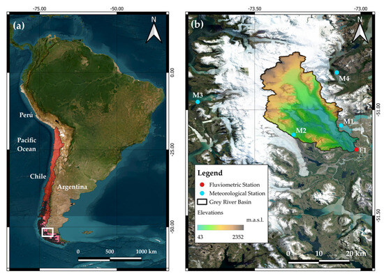
Figure 1.
(a) Location of Chile (red) and study area (white box) in South America, and (b) Lake Grey basin elevations and the location of meteorological (cyan dots) and fluviometric (red dot) stations.
The monthly temperature varies between −4 °C and 5 °C, while annual precipitation reaches 1200 mm. In wet and dry years, the highest flows occur between November and April because of snowmelt from headwater snowdrifts, while the lowest runoff is observed between June and September [46]. Runoff from the basin is linked to the melting of the Grey Glacier, representing a glacial regime [42], as shown in Figure 2.
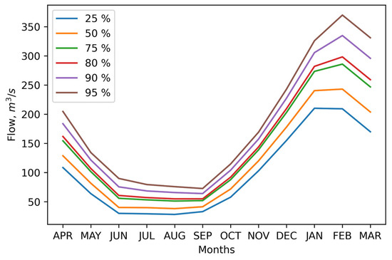
Figure 2.
Grey River seasonal variation curve.
The main channel of the Grey River is 20 km long and originates at the southern end of Lake Grey. This lake resembles an inland fjord due to its shape and dimensions, with a main axis of 16 km long and an average width of 2 km. Lake Grey is fed by a snowdrift located at its northern head [40], the thaw front of which is more than 20 m high and descends into the lake’s waters. The snowdrift is one of the numerous tributaries of the Southern Patagonian Ice Field. The surface area of the lake is about 38.6 km2 [39], and its waters are turbid due to glacial silt. At its southern end, it receives the Avutardas River, which drains from Lake Pingo, also fed by snowdrift [47].
2.2. Hydroclimatic Data
This study analyzed climatic and hydrological variables for the Grey River basin, including precipitation, mean temperature, potential evapotranspiration (PET, calculated according to the method of Hargreaves and Samani [48]) over 1979–2020, and flow over 1981–2020. These datasets originate from the CAMELS-CL database [49,50] and they are complemented with information from the Dirección General de Aguas (DGA) database (https://dga.mop.gob.cl/, accessed on 10 January 2025). Additionally, the wind speed at 5 m elevation in the zone was analyzed using the database of the Explorador Eólico from the Ministerio de Energía of Chile, which offers gridded information with a spatial resolution of 1 km (https://eolico.minenergia.cl/inicio, accessed on 10 January 2025). The evaluation period varied between 1980 and 2024, and the data were interpolated and weighted across the basin. The database of the Explorador Eólico has been validated in previous studies [51]. Table 1 shows the details of each gauging station used.

Table 1.
Information from Lake Grey basin’s meteorological and fluviometric stations.
2.3. Climate Indices
2.3.1. Antarctic Oscillation Index (AAO)
The Southern Annular Mode (SAM), which is often referred to as the Antarctic Oscillation (AAO) [52], has strong effects on the climate systems at high and middle latitudes of the Southern Hemisphere [53]. The AAO is a leading mode of midlatitude circulation variability, representing a seesaw-like mass change between mid- and high latitudes. The positive phase of the SAM is characterized by lower anomalous air pressures over the Antarctic along with abnormal pressure over the middle latitudes. With changes in air pressure distribution, changes in the strength and position of the westerly winds can occur. In the positive SAM phase, the westerly winds are stronger and move poleward, while the westerly winds weaken in the negative phase and move toward the equator. The leading mode of sea-level pressure variability in the extratropics statistically defines the AAO index [54], which is the normalized zonal mean sea level pressure (SLP) difference between −40° and −70° [55].
2.3.2. El Niño—Southern Oscillation Index (ENSO)
The El Niño—Southern Oscillation (ENSO) is an ocean–atmosphere phenomenon in which the cooler equatorial eastern Pacific Ocean warms once every 2 to 7 years [56,57]. This phenomenon is the dominant interannual mode of variability in tropical meteorology [58]. The increase in equatorial eastern Pacific sea surface temperature (SST) is attributed to the weakening of the easterly trade winds that result in warm water from the western Pacific moving to the east [59]. This phenomenon has two phases: El Niño, characterized by increased SST (warm phase), higher rainfall, and weaker winds, and La Niña, characterized by decreased SST (cold phase), reduced rainfall, and stronger winds [60,61]. ENSO oceanic indices are determined using SST anomalies averaged over the east-central equatorial region. Indices that are commonly used to classify ENSO events include regional SST indices (i.e., El Niño 4, El Niño 3.4, El Niño 3, and El Niño 1 + 2) [57].
El Niño 1 + 2 Sea Surface Temperature Index (ENSO)
According to the NOAA, this index monitors ENSO conditions in the far eastern tropical Pacific. The El Niño 1 + 2 Index region is between −80° and −90° and 0° to −10° [62]. It is especially relevant for South American countries such as Ecuador, Peru, and Chile [63], where it influences fishing, agriculture, and rainfall patterns and has a strong connection with fire weather conditions in central Chile [64]. The data for this index are available at https://www.ncei.noaa.gov/access/monitoring/enso/sst (accessed on 31 October 2024).
El Niño 3 Sea Surface Temperature Index (ENSO)
The El Niño 3 region is broader than El Niño 1 + 2, extending further westward into the Pacific. The El Niño 3 Index has been used to study the long-term behavior of ENSO and its impacts. It covers the area between latitudes 5° and −5°, and between longitudes −150° and −90° [62]. The data for this index are available at https://www.ncei.noaa.gov/access/monitoring/enso/sst (accessed on 31 October 2024).
El Niño 3.4 Sea Surface Temperature Index
The El Niño 3.4 Index, which is calculated over an area in the eastern Pacific between −120° and −170° longitude and 5° to −5° latitude [65,66,67], provides monthly data beginning in January 1950. This index is significant for understanding the effects of ENSO in Chile, especially regarding changes in precipitation patterns. The data for this index are available at https://www.ncei.noaa.gov/access/monitoring/enso/sst (accessed on 31 October 2024).
El Niño 4 Sea Surface Temperature Index
The El Niño 4 index covers the region between 160° and −150° latitudes and 5° and −5° longitudes [58]. It is key to assessing how ocean temperatures affect rainfall and trade wind patterns in this area. The data for this index is available at https://www.ncei.noaa.gov/access/monitoring/enso/sst (accessed on 31 October 2024).
2.3.3. Pacific Decadal Oscillation Index (PDO)
The Pacific Decadal Oscillation Index (PDO) is defined as the principal component of monthly SST variability in the North Pacific poleward 20° [68]. The PDO predominantly varies on decadal-to-multidecadal timescales [69]. Extreme PDO patterns are marked by widespread variations in the Pacific Basin and North American climates. The extreme phases of the PDO have been classified as being warm or cool, as defined by the ocean temperature in the northeast and the tropical Pacific Ocean [70,71].
2.4. Statistical Analysis
Statistical analysis of flow, temperature, potential evapotranspiration, and wind speed variables was performed at various temporal scales: monthly, seasonal, and pluri-annual aggregations (3-year, 7-year, and 10-year). For each aggregation, trends in the time series were evaluated, along with the magnitude of observed changes. Additionally, their correlations with large-scale climatic phenomena, including AAO, ENSO, and PDO, were analyzed.
2.4.1. Trend Analysis
The Mann–Kendall test (MK) [72,73] was applied to each time series of each variable, determining the direction of the trend for an increase, decrease, or neutrality [74]. This is a non-parametric test to detect monotonic trends within a time series. Since most of the hydrodynamic data present bias, it is convenient to use a non-parametric test for evaluation [75]. This type of test has been used for the evaluation of different variables such as flow, temperature, and potential evapotranspiration, among others [76,77]. The Mann–Kendall test statistic (S) is computed according to Equations (1) and (2):
where N is the length of the dataset and and denote the data values at time i and j, respectively. While the negative value of S indicates a decreasing trend, the positive value indicates an increasing trend [78]. The hydrometeorological time series trend slope magnitude is obtained by Sen’s slope estimation [79], which is a robust and non-parametric slope estimation accepted as an alternative to the least squares method [74]. One of the assumptions of the MK test is that the observations are independent of each other, meaning there is no serial correlation [80]. However, hydrological time series frequently infringe this assumption in practice. To address this issue, we first evaluate all series for serial correlation using the Ljung–Box test [81]. When significant autocorrelation was detected (p < 0.05), we applied the Hamed–Rao modified MK test, which incorporates a variance correction to account for persistent data structures [82].
In addition, the Pettitt test [83] was applied as a complement to MK test. This non-parametric test does not assume any distribution of the input data [84] and identifies the time mark or shift point where the change in the time series occurs [78,85]. The statistics are given as follows in Equations (3) and (4):
Pettitt’s () test statistics are commonly applied to determine how many times the first segment of the time series exceeds the second data segment. Mathematically, the series is non-homogeneous when the calculated values exceed the test statistic () [84].
2.4.2. Correlation Analysis
Spearman’s rank-order correlation () analysis is a non-parametric method that does not require any assumptions about data distribution [86]. This method measures the strength and direction of monotonic association between two variables [87]. It assesses how satisfactory the relationship between two variables can be described using a monotonic function [88]. It has been used in several hydrological studies, such as the relationship between precipitation and ENSO phenomena [89] and the correlation between erosion in saline rangelands and precipitation [90]. The Spearman correlation coefficient is the Pearson correlation coefficient between ranked variables and is given by Equation (5):
where denotes the Spearman’s rank correlation applied to the variables and , and are covariances of the ranked variables, N is the sample size, and are the standard deviations of the ranked variables. The statistics vary between −1 and 1, and a value of 1 or −1 means the paired data have a perfect monotonic relationship [91].
2.5. Principal Component Analysis (PCA)
Principal component analysis (PCA) is a classical statistical method that can reduce the high dimensionality of analyzed data while retaining most of the variation in the dataset through the orthogonal linear transformation of the correlated variables into a small number of uncorrelated variables called principal components [92]. This method has been applied in several hydrological studies, especially in groundwater [93], water quality [94,95,96], and precipitation analysis [97,98]. For more details about the application of the method, we recommend reviewing [99].
A principal component analysis was included to assess the most significant relationships between hydroclimatic variables and AAO, ENSO, and PDO phenomena. All climatic phenomena, including all ENSO regions (i.e., ENSO 1 + 2, 3, 3.4, and 4) were considered to determine which has the greatest influence on the analyzed climatic variables, following the methodology outlined in [97]. The analysis was performed using FactoMineR package (v2.8) in R. The climate indices and target variables (i.e., flow, wind, and precipitation) were standardized (z-scores) to account for unit differences, and the missing data were removed via listwise deletion.
2.6. Time-Varying Correlation
A sliding window analysis was employed to assess the correlation between each variable and the climatic phenomenon considered in this study using the Pearson correlation coefficient (r). For this purpose, the hydRopclim tool [100] was used, specifically, the indexcorrl function, which generates seasonal indices based on monthly hydroclimatological data and compares them with the AAO, ENSO, and PDO indices. The objective of this tool is to check predictions and find spatiotemporal patterns [97]. Based on the literature, we selected a 3-year window for AAO [101], 7-year window for ENSO [102], and 10-year window for PDO [103].
2.7. Wavelet and Coherence Analysis
To analyze the periodicity of the AAO, ENSO, and PDO indices with hydroclimatic variables, we employed wavelet analysis. For a comprehensive overview of wavelet theory and application, readers are directed to [104,105,106,107,108]. A wavelet transformation is a strong mathematical signal processing tool like the Fourier transformation, with the ability to analyze both stationary and nonstationary data and to produce both time and frequency information with a higher resolution, which is not available from traditional transformations [109]. Wavelet analysis aims to determine the frequency content of a signal and to assess and determine the temporal variation of this frequency content [110].
Each climatic phenomenon considered in this study was analyzed using the wavelet transform (WT), a method that examines frequency and phase variations over time across multiple scales simultaneously [111]. Additionally, cross-wavelet transform (XWT) and wavelet coherence (XWC) analyses were employed to detect significant variations in the relationships between hydrometeorological time series and large-scale phenomena. The XWT identifies shared periodicities between two time series and assesses temporal lags between their oscillation peaks, while the XWC quantifies the strength of these associations through correlation coefficients and significance testing [112]. In all cases, the significance level used is 0.05.
3. Results
3.1. Analysis of Hydroclimatic Variables
The time series of all the hydroclimatic variables analyzed in this study can be seen in Figure 3. A visual inspection suggests that there are no significant trends, except for the flow (Figure 3e). Additionally, it is possible to note a reduction in extreme values in the series of mean temperature (Figure 3c) and potential evapotranspiration (Figure 3d), in contrast to wind, which has shown an increase in extreme events (Figure 3a).
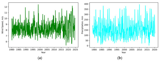
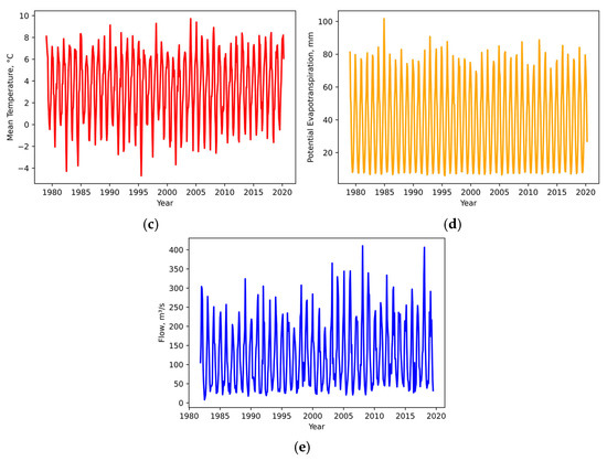
Figure 3.
Analyzed time series of (a) wind speed, (b) precipitation, (c) mean temperature, (d) potential evapotranspiration, and (e) flow.
In addition to the series in Figure 3, Table 2 shows the statistics for each of the variables analyzed. Both flow and precipitation (Prec) exhibit significant dispersion, as indicated by the comparison of their mean values, standard deviations, and extreme values. Likewise, the positive skewness coefficient suggests that the data generally tend to cluster around higher values. This pattern is also observed, although to a lesser degree, in potential evapotranspiration (PET) and wind speed. In contrast, the mean temperature (Mean Temp) shows an opposite trend. It exhibits narrower ranges of variation and a negative skewness coefficient, indicating that its values are more concentrated at the lower end of their distributions.
Table 2.
Reference statistics of precipitation (Prec), mean temperature (Mean Temp), potential evapotranspiration (PET), wind speed, and flow. Max represents the maximum, Min the minimum, STD the standard deviation, SC the skewness coefficient, and # the number of data.
When analyzing Table 2, it is possible to note that both flow and precipitation show high variability when reviewing their range and standard deviation (flow shows an average of 123.49 m3/s and a standard deviation of 83.93 m3/s, and precipitation shows an average of 153.12 mm and a standard deviation of 73.53 mm). In addition, both present a positive asymmetry, indicating that both variables are affected by extreme events. In the case of temperature, there are slight asymmetries (skewness coefficient of −0.27) and low dispersion (standard deviation of 3.04 °C). With the extreme values, a cold climate with moderate fluctuations is observed. The wind speed shows moderate variation (standard deviation of 1.20 m/s) in a consistently windy environment (maximum of 12.40 m/s).
3.2. Trends in Hydroclimatic Variables
The result varies when analyzing the trends of each variable considered in this study. Considering the complete time series, the flow series exhibits an increasing trend (MK test, p-value = 0.02), with a shift point detected in November 2002. However, no trends were identified when analyzing the rest of the variables. To assess changes in each variable, the Mann–Kendall test was supplemented with Sen’s slope on an annual basis, as shown in Table 3. This analysis reveals that only the flow, precipitation, and wind speed exhibit significant changes. All other variables have Sen’s slopes close to 0. The rest of the trend results and p-values are presented in Table S1.
Table 3.
Sen’s slope values for each hydroclimatic variable.
To obtain a more detailed analysis, the time series are grouped by season, considering summer (January to March), autumn (April to June), winter (July to September), and spring (October to December), according to the seasons in the study area. The seasonal trend analysis reveals similar results to those previously mentioned, as shown in Figure 4. The flow shows increasing trends in summer (p-value = 0.005), autumn (p-value = 0.001), and winter (p-value = 0.019), while the rest of the time, it does not change. On the other hand, wind speed shows a decreasing trend in autumn (p-value = 0.003) and winter (p-value = 0.020). As was the case when analyzing the trends of the complete series, the rest of the variables show no changes. The p-values for each of the considered variables are shown in Tables S2–S6 for flow, precipitation, mean temperature, potential evapotranspiration, and wind speed, respectively.
Figure 4.
Trends for each season for the variables precipitation (cyan), mean temperature (red), potential evapotranspiration (orange), wind speed (green), and flow (blue).
A monthly analysis of each variable yields similar results to those described above. The flow rate shows an increasing trend in April (p-value = 0.010), May (p-value = 0.008), June (p-value = 0.008), July (p-value = 0.019), August (p-value = 0.041), September (p-value = 0.012), and December (p-value = 0.019), with a strong influence from the winter months, as illustrated in Figure 5. Additionally, the potential evapotranspiration (PET) shows an increasing trend only in February (p-value = 0.013). In contrast, the wind speed shows a decreasing trend in June (p-value = 0.002) and an increasing trend in January (p-value = 0.030). In all other cases, the result was “no trend,” which implies that the hydroclimatic variables are only increasing when performing a monthly discretization of the time series. The p-values for each of the variables considered are shown in Tables S7–S11 for flow, precipitation, mean temperature, potential evapotranspiration, and wind speed, respectively.
Figure 5.
Trends for each month for the variables precipitation (cyan), mean temperature (red), potential evapotranspiration (green), wind speed (green), and flow (blue).
3.3. Relationship Between Hydroclimatic Variables and Major Climate Phenomena
3.3.1. Correlation Analysis
Spearman’s rank correlation testing was performed to analyze the relationship between hydroclimatic variables and major climate phenomena. This analysis assessed the association between the variables studied and three key climatic drivers: AAO, ENSO, and PDO. Figure 6 shows the results of this procedure. When analyzing the results globally, the highest correlation values consistently align with the AAO phenomenon (r = 0.1497 for flow, p-value = 0.0014). On the other hand, the variables show a neutral correlation with the El Niño 1 + 2 Index, being the least representative for this zone (maximum r = 0.0521 for PET, p-value = 0.0136). Upon examining the variables individually, precipitation and potential evapotranspiration show the lowest correlation values among all the analyzed variables, while the flow rate and mean temperature show the strongest positive correlation with AAO. Finally, all variables show weak correlations with PDO, the highest being the relationship with wind speed (r = 0.0871, p-value = 0.0437). The results of Spearman’s correlation and p-value between each climate variable and large-scale climatic phenomenon are shown in Table S12.
Figure 6.
Correlation between ENSO, AAO, and PDO phenomena with flow, precipitation (Prec), mean temperature (Mean Temp), potential evapotranspiration (PET), and wind speed.
3.3.2. Principal Component Analysis (PCA)
The results of the PCA between the climatic variables and the analyzed phenomena are presented in Figure 7. It can be observed that for flow (Figure 7a), precipitation (Figure 7b), and wind speed (Figure 7c), ENSO 3.4 is the most representative index within the El Niño phenomenon. Because of this, in subsequent analyses, only this ENSO region was considered. Additionally, in all cases, the PDO appears to be the least influential long-term phenomenon on climate variables. In this context, the AAO exhibits the highest correlations, with direct correlations for flow (Figure 7a) and wind speed (Figure 7c) and an inverse relationship for precipitation (Figure 7b). Additionally, mean temperature and potential evapotranspiration exhibited a similar clustering pattern to that of flow.
Figure 7.
Projection of Antarctic Oscillation (AAO), El Niño—Southern Oscillation (ENSO), and Pacific Decadal Oscillation (PDO) indices into (a) flow, (b) precipitation, and (c) wind speed.
3.3.3. Time-Varying Correlation Between Climate Indices
An evaluation of the Pearson correlations between climatic phenomena and various climatic variables, such as flow, precipitation, average temperature, and potential evapotranspiration, was conducted using a moving window. For AAO, the analysis utilized a 3-year time window. Similarly, a 7-year was applied for ENSO (i.e., El Niño 3.4), while a 10-year window was used for PDO, given its classification as a large-scale phenomenon. The analysis results are presented in Figure 8, Figure 9 and Figure 10, corresponding to the AAO, ENSO, and PDO phenomena, respectively. For the AAO, it is possible to note a positive relationship of the phenomenon with the variables of flow, mean temperature, and potential evapotranspiration in the period around 2002, where the shift point was identified. In this period, positive Pearson correlations that exceeded the value of 0.5 were reached.
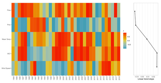
Figure 8.
Three-year moving correlation (Pearson) between AAO and flow, precipitation (Prec), mean temperature (Mean Temp), potential evapotranspiration (PET), and wind speed over 1980–2020.
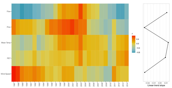
Figure 9.
Seven-year moving correlation (Pearson) between ENSO 3.4 and flow, precipitation (Prec), mean temperature (Mean Temp), potential evapotranspiration (PET), and wind speed over 1980–2020.
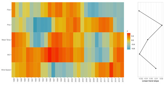
Figure 10.
Ten-year moving correlation (Pearson) between PDO and flow, precipitation (Prec), mean temperature (Mean Temp), potential evapotranspiration (PET), and wind speed over 1980–2020.
In the case of the relationship between climatic variables and ENSO 3.4 (Figure 9), with an analysis window of 7 years, it is possible to note that precipitation has the highest correlation (r > 0.4). Conversely, both temperature and potential evapotranspiration show correlations close to zero with this large-scale phenomenon.
Finally, for the case of the PDO, it is potential evapotranspiration and wind speed that present the highest correlations (r > 0.4), coinciding with the period of 1997 and 2014, respectively. When analyzing the relationship between the variables and the AAO (Figure 8), similarities can be seen in the variability of the mean temperature (Mean Temp) and PET, as these variables are strongly interconnected. This relationship also holds for large-scale phenomena, such as ENSO and PDO, which occur over larger timescales, as shown in Figure 9 and Figure 10, respectively. Additionally, a similarity between flow and mean temperature can be observed, as evidenced by the Spearman’s correlations (Figure 6) and the analyzed windows in Figure 8, Figure 9 and Figure 10 for AAO, ENSO 3.4, and PDO.
3.3.4. Wavelet Analysis
Figure 11 shows the cross-wavelet, wavelet coherence, and the mean coherence peaks analysis between the flow data and the AAO phenomenon. A significant power correlation is observed for phenomena with a 1-year frequency (Figure 11a). In most cases, the arrows point to the left, indicating a lag associated with the coincidence of flow peaks with the negative phase of the AAO. However, the phase correlation extends to phenomena with frequencies of up to 2 years, with 2000–2005 being the most relevant and to a lesser extent the periods 1990–1995 and 2010–2015 (Figure 11b), indicating a consistent phase relationship over longer timescales. This coincides with that shown in Figure 7c, where the coherence peaks are in 1-year and 2-year events. In addition, and to a lesser extent, there is consistency between 1995 and 2000 between the flow and AAO (Figure 11b).
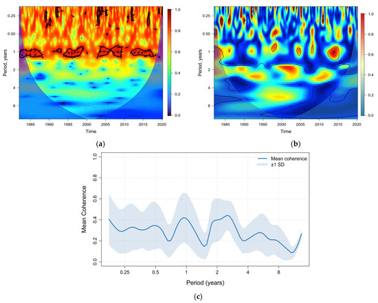
Figure 11.
(a) Cross-wavelet transform, (b) coherence wavelet, and (c) mean coherence peaks for wavelet coherence between flow and AAO.
Figure 12 shows the relationship between precipitation and the ENSO 3.4 index. Power correlations are observed around the 1997 and 2014 periods (Figure 12a). This power correlation is also reflected in the coherence (Figure 12b), revealing additional regions of importance at 3- and 4-year frequencies. When analyzing Figure 12c, it is possible to notice that the coherence peaks occur at 2- and 4-year frequencies, coinciding with the ENSO of 1982 and 1997.
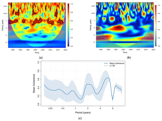
Figure 12.
(a) Cross-wavelet transform, (b) coherence wavelet, and (c) mean coherence peaks for wavelet coherence between precipitation and ENSO 3.4.
4. Discussion
In this study, we analyzed the trends of long-term climatic variables, such as precipitation, potential evapotranspiration, mean temperature, wind speed, and streamflow, of the Grey River basin in Chilean Patagonia. Additionally, we assessed the relation of these variables with large-scale phenomena, including AAO, ENSO, and PDO. Trend assessments were performed for the full time series, as well as disaggregated by month and season, to capture both long-term and intra-annual patterns. The influence of large-scale climate modes on local climatic variability was explored using wavelet analysis and moving window correlation techniques, allowing the evaluation of the temporal and frequency-dependent relationships.
The results in Table 2 reveal a marked variability in streamflow and precipitation, suggesting a hydrological regime strongly influenced by extreme events. This high variability, evidenced by the large standard deviations and positive skewness, is characteristic of systems where intense events can affect the hydrological response. In contrast, temperature shows low dispersion and a slight negative skewness, indicating relatively stable thermal conditions and a predominantly cold climate, with a few occurrences of extreme temperature values. This reflects the geography of the study area. Additionally, wind speed values indicate a consistently windy environment with moderate variability. The presence of steady winds, occasionally reaching higher intensities (up to 12.40 m/s), may significantly influence processes such as evaporation and atmospheric mass transport. Additionally, precipitation records (Figure 3b) exhibit a similar temporal pattern to that presented by Garreaud [33], who identified the 2016 rainfall deficit as the most severe drought on record in western Patagonia (between −40° and −48° latitude and −71° and −76° longitude). Furthermore, it is possible to note that the series shares a common period from 1980 to 2020.
In analyzing the trends in the complete series, we found changes only in flow. It exhibits a positive trend, as determined by the MK test, with a shift point identified in November 2002. This shift has been detected by several studies, like Douglass and Knox [113], who identified a global change in ocean heat content (OHC) during 2001 and 2002, Bode et al. [114], who reported a change in plankton to the north of Spain due to the combined effects of hydrography and nutrient availability, and Rahman et al. [115], who identified changes in 2001 in the abundance of Pacific cod and chub mackerel in Asia, as well as in the temperatures in the northern and eastern Japan Sea. Additionally, he observed similar changes in the East China Sea in 2002. However, this had not been identified in climatic variables within glacial basins in the southern hemisphere. The remaining variables display no significant trends. For flow, 2003 stands out as the year with the highest temperatures recorded since 1990, coupled with extreme wind events during these months [116]. These conditions contributed to ice melting in the region, resulting in a gradual increase in the flow of the Grey River. Furthermore, as highlighted in Table 3 and Figure 3, the increase in flow is approximately 0.710 m3/s, representing 10% of the minimum flow (Table 2) recorded in the Grey River during the period analyzed.
A seasonal analysis of the climatic variables (Figure 4) reveals that only flow and wind speed show changes in their trends. Flow shows variations during summer, autumn, and winter, corresponding to the glacial hydrological regime of the basin (Figure 2), where the highest values are recorded during periods of low water availability. In contrast, wind speed tends to decrease in autumn and winter, the seasons with the toughest climatic conditions in the study area. The observed changes persist when trends are analyzed monthly. However, some months show variations in additional variables. For instance, potential evapotranspiration increases in February, and wind speed decreases in June. Notably, even when the variables are temporally disaggregated, flow and wind speed remain the ones with the most significant changes. Knowing the trends of these variables can provide valuable information to decision-makers and stakeholders [117].
Figure 6 shows that when analyzing the complete series of hydroclimatic variables, stronger correlations are observed with the AAO. Similarly, the ENSO 3.4 index exhibits a notable association with the data, consistent with findings from previous studies on the Chilean region [118]. Conversely, the analysis indicates no significant correlation with the PDO. This lack of association may be attributed to the need for analyzing such phenomena over timeframes of at least a decade [103].
After analyzing the relationships between climatic variables and long-term phenomena, it was identified that flow, precipitation, and wind speed are the most representative variables for the study area. This selection considers that the behavior of mean temperature and potential evapotranspiration closely follows that of flow. In this context, through PCA, it was observed that in all cases, ENSO 3.4 was the most influential El Niño index in the study area (Figure 7). These results coincide with the findings on the trends in the climatic variables, the ones with the greatest variation being the flow rate and wind speed. Additionally, the AAO is the most relevant phenomenon, showing a direct relationship with flow (Figure 7a) and wind speed (Figure 7c) and an inverse relationship with precipitation (Figure 7b). Finally, in all cases, the PDO is the least relevant phenomenon in analyzing climatic variables. However, it should be noted that this study is limited by the 40-year data record, which may be insufficient/inadequate to establish conclusions about the influence of PDO in the study area.
Figure 8, Figure 9 and Figure 10 illustrate the relationships between AAO, ENSO 3.4, and PDO with various climatic variables, highlighting notable differences over time. Firstly, the AAO (Figure 8) shows periods of moderate and negative correlation, around 0.5. However, this pattern does not extend to precipitation, which shows only a moderate negative correlation of −0.5. This relationship aligns with atmospheric dynamics, as during the positive phase of the AAO, the westerly wind belt shifts southward, reducing the influence of frontal systems in the region and consequently decreasing precipitation. Additionally, it is possible to note that flow, mean temperature, and PET present a high positive correlation (r > 0.5) in the period between 1995 and 2000, coinciding with one of the most extreme climatic events of recent times [115,119].
Conversely, in the negative phase of the AAO, the westerly wind belt moves to more northerly latitudes, enhancing the likelihood of rainfall in Magallanes y la Antártica Chilena, due to an increase in cold fronts and low-pressure systems. ENSO phenomenon (Figure 9) exhibits varying behaviors depending on the variable analyzed. For instance, in the case of precipitation, negative Pearson correlations nearing −0.8 were observed in the early 1990s, transitioning to positive correlations until approximately 0.4 during the period from 1994 to 1998, coinciding with the 1997 ENSO phenomenon [120,121]. When evaluating the correlation between hydroclimatic variables and the PDO (Figure 10) using a 10-year moving window, stronger correlations are observed with the flow and precipitation. These periods were identified in previous studies as ENSO events of great relevance, and an overlap in the effects of large-scale phenomena can be found [97,122].
A strong relationship is observed between the analyzed climatic variables and the phenomena considered in this study (Figure 11 and Figure 12). Notably, there is a precise alignment with major events, particularly El Niño in 1997 [120,123], 2009 [124], and 2014 [122], as well as an overlapping relationship between the effects of AAO, ENSO, and PDO. Additionally, despite the varying frequencies of large-scale phenomena, stronger power relationships are observed at a 1-year frequency (Figure 11a and Figure 12a). In contrast, the coherence analysis reveals a consistent relationship for higher-frequency events (Figure 11b and Figure 12b). These results coincide with those presented by Mendes and Cavalcanti [119], where they related the persistent anticyclones (blocking events) in South America with the AAO, identifying the same periods described in this study. Additionally, Rahman et al. [115] identified breaks in the AAO in the years 1987, 1995, and 2014, coinciding with what is shown in Figure 11b.
In general, an out-of-phase relationship can be observed with the phases of the AAO, ENSO, and PDO phenomena, as indicated by the direction of the arrows in Figure 11 and Figure 12. This occurs because the warm phases of the analyzed phenomena lead to a decrease in precipitation and streamflow in Patagonia, contrary to what happens at lower latitudes [125].
5. Conclusions
This study provides an evaluation of the relationships between major climatic phenomena and hydroclimatic variables in the Grey River basin, a glacially fed watershed located in Chilean Patagonia. Through a combination of statistical techniques, including trend analysis, correlation tests, principal component analysis, and wavelet coherence analysis, this research reveals that the basin’s hydrology is significantly influenced by large-scale climate variability, particularly the AAO and ENSO. The streamflow trend shows a statistically significant increase, especially during winter and spring, likely driven by increased glacial melt in response to rising temperatures and extreme wind events observed in 2002. The AAO emerged as the dominant climatic driver in the region, showing strong associations with streamflow and wind patterns, while ENSO 3.4 demonstrated a notable influence over precipitation variability, especially during major El Niño episodes (e.g., 1997, 2009, and 2014). In contrast, PDO had a relatively minor effect on the basin’s hydroclimatic behavior. These findings suggest that the interplay between local glacial dynamics and global atmospheric phenomena governs the temporal variability in water availability in this basin. As climate change continues to alter the behavior of these large-scale phenomena, understanding their impact becomes essential for anticipating future water resource scenarios in Patagonia. This study is a preliminary contribution to Chile’s Water Framework Law (Law No. 21455), which creates a legal framework for the country to address climate change mitigation and adaptation in the long term and thus comply with its international commitments. To better understand the effects of hydrological processes on the melting of Grey Glacier, the use of glacio-hydrological modeling in the basin is proposed for future work, along with improved spatial and temporal resolution of hydroclimatological information.
Supplementary Materials
The following supporting information can be downloaded at https://www.mdpi.com/article/10.3390/w17131895/s1, Table S1: Trends in the complete series of climatic variables according to Mann–Kendall tests and their respective p-values; Table S2: Seasonal trends for flow according to Mann–Kendall tests and their respective p-values; Table S3: Seasonal trends for precipitation according to Mann–Kendall tests and their respective p-values; Table S4: Seasonal trends for mean temperature according to Mann–Kendall tests and their respective p-values; Table S5: Seasonal trends for potential evapotranspiration according to Mann–Kendall tests and their respective p-values; Table S6: Seasonal trends for wind speed according to Mann–Kendall tests and their respective p-values; Table S7: Monthly trends for flow according to Mann–Kendall tests and their respective p-values; Table S8: Monthly trends for precipitation according to Mann–Kendall tests and their respective p-values; Table S9: Monthly trends for mean temperature according to Mann–Kendall tests and their respective p-values; Table S10: Monthly trends for potential evapotranspiration according to Mann–Kendall tests and their respective p-values; Table S11: Monthly trends for wind speed according to Mann–Kendall tests and their respective p-values; Table S12: Spearman’s correlation and p-values between climate variables and large-scale phenomena.
Author Contributions
Conceptualization, P.F.-A. and L.R.-L.; methodology, P.F.-A.; software, P.F.-A.; validation, L.R.-L., L.B. and F.F.; formal analysis, P.F.-A.; investigation, P.F.-A.; resources, P.F.-A., L.R.-L., L.B. and F.F.; data curation, P.F.-A.; writing—original draft preparation, P.F.-A.; writing—review and editing, L.R.-L., L.B. and F.F.; visualization, P.F.-A.; supervision, L.B. and F.F.; project administration, L.R.-L., L.B. and F.F.; funding acquisition, P.F.-A. and L.R.-L. All authors have read and agreed to the published version of the manuscript.
Funding
The APC was funded by Project ANID/FOVI240030.
Data Availability Statement
Request from the corresponding author.
Acknowledgments
All authors’ thanks to Project ANID/FOVI 240030. P.F-A. thanks the Vicerrectoría de Investigación y Doctorados Fondo USS-FIN-24-PASD-14. F.F. thanks to CNES through the TOSCA SWOT WHYGHS program.
Conflicts of Interest
The authors declare that they have no conflicts of interest related to this study.
References
- Schäffer, A.; Groh, K.J.; Sigmund, G.; Azoulay, D.; Backhaus, T.; Bertram, M.G.; Carney Almroth, B.; Cousins, I.T.; Ford, A.T.; Grimalt, J.O.; et al. Conflicts of Interest in the Assessment of Chemicals, Waste, and Pollution. Environ. Sci. Technol. 2023, 57, 19066–19077. [Google Scholar] [CrossRef] [PubMed]
- Afifa; Arshad, K.; Hussain, N.; Ashraf, M.H.; Saleem, M.Z. Air Pollution and Climate Change as Grand Challenges to Sustainability. Sci. Total Environ. 2024, 928, 172370. [Google Scholar] [CrossRef] [PubMed]
- Schmidt, C.; Kühnel, D.; Materić, D.; Stubenrauch, J.; Schubert, K.; Luo, A.; Wendt-Potthoff, K.; Jahnke, A. A Multidisciplinary Perspective on the Role of Plastic Pollution in the Triple Planetary Crisis. Environ. Int. 2024, 193, 109059. [Google Scholar] [CrossRef]
- Bachmann, M.; Zibunas, C.; Hartmann, J.; Tulus, V.; Suh, S.; Guillén-Gosálbez, G.; Bardow, A. Towards Circular Plastics within Planetary Boundaries. Nat. Sustain. 2023, 6, 599–610. [Google Scholar] [CrossRef]
- Mahmood, A.; Farooq, A.; Akbar, H.; Ghani, H.U.; Gheewala, S.H. An Integrated Approach to Analyze the Progress of Developing Economies in Asia toward the Sustainable Development Goals. Sustainability 2023, 15, 13645. [Google Scholar] [CrossRef]
- Ihsan, F.R.; Bloomfield, J.G.; Monrouxe, L.V. Triple Planetary Crisis: Why Healthcare Professionals Should Care. Front. Med. 2024, 11, 1465662. [Google Scholar] [CrossRef]
- Rezapouraghdam, H.; Hidalgo-Garcia, D.; Karatepe, O.M. Rising Temperatures and Sinking Hopes: An in-Depth Analysis of the Interplay between Climate Change, Land Use Patterns, and the Desiccation of a Global Biosphere Reserve. Environ. Dev. 2024, 52, 101084. [Google Scholar] [CrossRef]
- Balaram, V. Combating Climate Change and Global Warming for a Sustainable Living in Harmony with Nature. J. Geogr. Res. 2023, 6, 1–17. [Google Scholar] [CrossRef]
- Tzanakakis, V.A.; Paranychianakis, N.V.; Angelakis, A.N. Water Supply and Water Scarcity. Water 2020, 12, 2347. [Google Scholar] [CrossRef]
- Revich, B.A. The significance of green spaces for protecting health of urban population. Health Risk Anal. 2023, 2, 168–185. [Google Scholar] [CrossRef]
- Kreibich, H.; Van Loon, A.F.; Schröter, K.; Ward, P.J.; Mazzoleni, M.; Sairam, N.; Abeshu, G.W.; Agafonova, S.; AghaKouchak, A.; Aksoy, H.; et al. The Challenge of Unprecedented Floods and Droughts in Risk Management. Nature 2022, 608, 80–86. [Google Scholar] [CrossRef]
- Susmaa, K.S.; Jeni, J.M.; Prasanna, A.; Manikandavelu, D.; Sona, B.R.; Masilan, K.; Mahalakshmi, B. Exploring the Vital Role of Coral Disease in Coral Reef Sustainability: A Comprehensive Analysis. Asian J. Environ. Ecol. 2024, 23, 32–43. [Google Scholar] [CrossRef]
- Wudil, A.H.; Usman, M.; Rosak-Szyrocka, J.; Pilař, L.; Boye, M. Reversing Years for Global Food Security: A Review of the Food Security Situation in Sub-Saharan Africa (SSA). Int. J. Environ. Res. Public Health 2022, 19, 14836. [Google Scholar] [CrossRef] [PubMed]
- IPCC. Impacts of 1.5 °C Global Warming on Natural and Human Systems. In Global Warming of 1.5 °C: IPCC Special Report on Impacts of Global Warming of 1.5 °C above Pre-Industrial Levels in Context of Strengthening Response to Climate Change, Sustainable Development, and Efforts to Eradicate Poverty; Cambridge University Press: Cambridge, UK, 2022; pp. 175–312. [Google Scholar]
- Panez, A.; Mansilla-Quiñones, P.; Olea Peńaloza, J. The Struggle for Water as a Source for Territorial Re-Existence in Chile: Rethinking the Agrarian Question in Latin America. Lat. Am. Perspect. 2024, 51, 163–183. [Google Scholar] [CrossRef]
- Jódar, J.; Urrutia, J.; Herrera, C.; Custodio, E.; Martos-Rosillo, S.; Lambán, L.J. The Catastrophic Effects of Groundwater Intensive Exploitation and Megadrought on Aquifers in Central Chile: Global Change Impact Projections in Water Resources Based on Groundwater Balance Modeling. Sci. Total Environ. 2024, 914, 169651. [Google Scholar] [CrossRef]
- Garreaud, R.D.; Alvarez-Garreton, C.; Barichivich, J.; Pablo Boisier, J.; Christie, D.; Galleguillos, M.; LeQuesne, C.; McPhee, J.; Zambrano-Bigiarini, M. The 2010–2015 Megadrought in Central Chile: Impacts on Regional Hydroclimate and Vegetation. Hydrol. Earth Syst. Sci. 2017, 21, 6307–6327. [Google Scholar] [CrossRef]
- Álamos, N.; Alvarez-Garreton, C.; Muñoz, A.; González-Reyes, Á. The Influence of Human Activities on Streamflow Reductions during the Megadrought in Central Chile. Hydrol. Earth Syst. Sci. 2024, 28, 2483–2503. [Google Scholar] [CrossRef]
- Salas-Bravo, S.; Araya-Piñones, A. Climate Change and Adaptive Capacity in the Community of Diaguitas, Chile: A Descriptive-Comparative Vision in Two Time Periods. Water Policy 2024, 26, 773–792. [Google Scholar] [CrossRef]
- Kim, Y.; Kim, S.; Jeong, H.; An, H. Quantitatively Defining Megadrought Based on Drought Events in Central Chile. Geomat. Nat. Hazards Risk 2022, 13, 975–992. [Google Scholar] [CrossRef]
- Alvarez-Garreton, C.; Pablo Boisier, J.; Garreaud, R.; Seibert, J.; Vis, M. Progressive Water Deficits during Multiyear Droughts in Basins with Long Hydrological Memory in Chile. Hydrol. Earth Syst. Sci. 2021, 25, 429–446. [Google Scholar] [CrossRef]
- Peña-Guerrero, M.D.; Nauditt, A.; Muñoz-Robles, C.; Ribbe, L.; Meza, F. Drought Impacts on Water Quality and Potential Implications for Agricultural Production in the Maipo River Basin, Central Chile. Hydrol. Sci. J. 2020, 65, 1005–1021. [Google Scholar] [CrossRef]
- Barra, R.O.; Chiang, G.; Saavedra, M.F.; Orrego, R.; Servos, M.R.; Hewitt, L.M.; McMaster, M.E.; Bahamonde, P.; Tucca, F.; Munkittrick, K.R. Endocrine Disruptor Impacts on Fish From Chile: The Influence of Wastewaters. Front. Endocrinol. 2021, 12, 611281. [Google Scholar] [CrossRef] [PubMed]
- Bopp, C.; Engler, A.; Jordan, C.; Jara-Rojas, R. What Is behind Water User Satisfaction with Irrigation Organizations’ Performance? An Empirical Analysis under Different Water Scarcity Conditions. Agric. Water Manag. 2024, 304, 109072. [Google Scholar] [CrossRef]
- Santiago, C.M.; Díaz, P.R.; Morales-Salinas, L.; Betancourt, L.P.; Fernández, L.O. Practices and Strategies for Adaptation to Climate Variability in Family Farming. An Analysis of Cases of Rural Communities in the Andes Mountains of Colombia and Chile. Agriculture 2021, 11, 1096. [Google Scholar] [CrossRef]
- Perez-Silva, R.; Castillo, M. Taking Advantage of Water Scarcity? Concentration of Agricultural Land and the Politics behind Water Governance in Chile. Front. Environ. Sci. 2023, 11, 1143254. [Google Scholar] [CrossRef]
- Willkofer, F.; Wood, R.R.; Ludwig, R. Assessing the Impact of Climate Change on High Return Levels of Peak Flows in Bavaria Applying the CRCM5 Large Ensemble. Hydrol. Earth Syst. Sci. 2024, 28, 2969–2989. [Google Scholar] [CrossRef]
- Cache, T.; Ramirez, J.A.; Molnar, P.; Ruiz-Villanueva, V.; Peleg, N. Increased Erosion in a Pre-Alpine Region Contrasts with a Future Decrease in Precipitation and Snowmelt. Geomorphology 2023, 436, 108782. [Google Scholar] [CrossRef]
- Manquehual-Cheuque, F.; Somos-Valenzuela, M. Climate Change Refugia for Glaciers in Patagonia. Anthropocene 2021, 33, 100277. [Google Scholar] [CrossRef]
- Bonneau, J.; Laval, B.; Mueller, D.; Hamilton, A. ArcticNet 2021 Annual Scientific Meeting Abstracts. Arct. Sci. 2022, 8, 3–152. [Google Scholar] [CrossRef]
- Jin, H.; Huang, Y.; Bense, V.F.; Ma, Q.; Marchenko, S.S.; Shepelev, V.V.; Hu, Y.; Liang, S.; Spektor, V.V.; Jin, X.; et al. Permafrost Degradation and Its Hydrogeological Impacts. Water 2022, 14, 372. [Google Scholar] [CrossRef]
- Minowa, M.; Skvarca, P.; Fujita, K. Climate and Surface Mass Balance at Glaciar Perito Moreno, Southern Patagonia. J. Clim. 2023, 36, 625–641. [Google Scholar] [CrossRef]
- Garreaud, R.D. Record-Breaking Climate Anomalies Lead to Severe Drought and Environmental Disruption in Western Patagonia in 2016. Clim. Res. 2018, 74, 217–229. [Google Scholar] [CrossRef]
- Rodríguez-López, L.; Bustos Usta, D.; Bravo Alvarez, L.; Duran-Llacer, I.; Lami, A.; Martínez-Retureta, R.; Urrutia, R. Machine Learning Algorithms for the Estimation of Water Quality Parameters in Lake Llanquihue in Southern Chile. Water 2023, 15, 1994. [Google Scholar] [CrossRef]
- Gong, D.Y.; Gao, Y.; Guo, D.; Mao, R.; Yang, J.; Hu, M.; Gao, M. Interannual Linkage between Arctic/North Atlantic Oscillation and Tropical Indian Ocean Precipitation during Boreal Winter. Clim. Dyn. 2014, 42, 1007–1027. [Google Scholar] [CrossRef]
- Zhang, K.; Qian, X.; Liu, P.; Xu, Y.; Cao, L.; Hao, Y.; Dai, S. Variation Characteristics and Influences of Climate Factors on Aridity Index and Its Association with AO and ENSO in Northern China from 1961 to 2012. Theor. Appl. Climatol. 2017, 130, 523–533. [Google Scholar] [CrossRef]
- Young, K.L.; Robert Bolton, W.; Killingtveit, Å.; Yang, D. Assessment of Precipitation and Snowcover in Northern Research Basins. Hydrol. Res. 2006, 37, 377–391. [Google Scholar] [CrossRef]
- Caloiero, T.; Caloiero, P.; Frustaci, F. Long-Term Precipitation Trend Analysis in Europe and in the Mediterranean Basin. Water Environ. J. 2018, 32, 433–445. [Google Scholar] [CrossRef]
- Sugiyama, S.; Minowa, M.; Schaefer, M. Underwater Ice Terrace Observed at the Front of Glaciar Grey, a Freshwater Calving Glacier in Patagonia. Geophys. Res. Lett. 2019, 46, 2602–2609. [Google Scholar] [CrossRef]
- Sugiyama, S.; Minowa, M.; Fukamachi, Y.; Hata, S.; Yamamoto, Y.; Sauter, T.; Schneider, C.; Schaefer, M. Subglacial Discharge Controls Seasonal Variations in the Thermal Structure of a Glacial Lake in Patagonia. Nat. Commun. 2021, 12, 6301. [Google Scholar] [CrossRef]
- Sugiyama, S.; Minowa, M.; Sakakibara, D.; Skvarca, P.; Sawagaki, T.; Ohashi, Y.; Naito, N.; Chikita, K. Thermal Structure of Proglacial Lakes in Patagonia. J. Geophys. Res. Earth Surf. 2016, 121, 2270–2286. [Google Scholar] [CrossRef]
- Medina, Y.; Muñoz, E. Analysis of the Relative Importance of Model Parameters in Watersheds with Different Hydrological Regimes. Water 2020, 12, 2376. [Google Scholar] [CrossRef]
- Kottek, M.; Grieser, J.; Beck, C.; Rudolf, B.; Rubel, F. World Map of the Köppen-Geiger Climate Classification Updated. Meteorol. Z. 2006, 15, 259–263. [Google Scholar] [CrossRef] [PubMed]
- Hüne, M.; Haro, D.; Davis, E.; Gutiérrez, D.; Anderson, C.B.; Sabat, P. Niche Overlap in Sympatric Introduced Trout from a Southern Patagonian River: Evidence from Stomach Contents and Stable Isotope Analysis. Panam. J. Aquat. Sci. 2022, 17, 304–312. [Google Scholar] [CrossRef]
- Lafon, A.; Silva, N.; Vargas, C.A. Contribution of Allochthonous Organic Carbon across the Serrano River Basin and the Adjacent Fjord System in Southern Chilean Patagonia: Insights from the Combined Use of Stable Isotope and Fatty Acid Biomarkers. Prog. Oceanogr. 2014, 129, 98–113. [Google Scholar] [CrossRef]
- Dirección General de Aguas. Diagnóstico y Clasificación de Los Cursos de Agua Según Objetivos de Calidad: Cuenca Del Río Serrano; Dirección General de Aguas: Santiago, Chile, 2004.
- Niemeyer, H. Hoyas Hidrográficas de Chile, Duodécima Región; Dirección General de Aguas: Santiago, Chile, 1982. [Google Scholar]
- Hargreaves, G.H.; Samani, Z.A. Samani Reference Crop Evapotranspiration from Temperature. Appl. Eng. Agric. 1985, 1, 96–99. [Google Scholar] [CrossRef]
- Alvarez-Garreton, C.; Mendoza, P.A.; Pablo Boisier, J.; Addor, N.; Galleguillos, M.; Zambrano-Bigiarini, M.; Lara, A.; Puelma, C.; Cortes, G.; Garreaud, R.; et al. The CAMELS-CL Dataset: Catchment Attributes and Meteorology for Large Sample Studies-Chile Dataset. Hydrol. Earth Syst. Sci. 2018, 22, 5817–5846. [Google Scholar] [CrossRef]
- Barría, P.; Sandoval, I.B.; Guzman, C.; Chadwick, C.; Alvarez-Garreton, C.; Díaz-Vasconcellos, R.; Ocampo-Melgar, A.; Fuster, R. Water Allocation under Climate Change: A Diagnosis of the Chilean System. Elementa 2021, 9, 00131. [Google Scholar] [CrossRef]
- Muñoz, R.C.; Falvey, M.J.; Arancibia, M.; Astudillo, V.I.; Elgueta, J.; Ibarra, M.; Santana, C.; Vásquez, C. Wind Energy Exploration over the Atacama Desert: A Numerical Model-Guided Observational Program. Bull. Am. Meteorol. Soc. 2018, 99, 2079–2092. [Google Scholar] [CrossRef]
- Tang, Y.; Duan, A. Asymmetry of the Antarctic Oscillation in Austral Autumn. Geophys. Res. Lett. 2023, 50, e2023GL105678. [Google Scholar] [CrossRef]
- Lee, D.Y.; Petersen, M.R.; Lin, W. The Southern Annular Mode and Southern Ocean Surface Westerly Winds in E3SM. Earth Space Sci. 2019, 6, 2624–2643. [Google Scholar] [CrossRef]
- Son, S.W.; Shin, J.H.; Park, H.S.; Choi, J. The Relationship Between the Zonal Index and Annular Mode Index in Reanalysis and CMIP5 Models. Asia-Pac. J. Atmos. Sci. 2022, 58, 117–126. [Google Scholar] [CrossRef]
- Nan, S.; Li, J. The Relationship between the Summer Precipitation in the Yangtze River Valley and the Boreal Spring Southern Hemisphere Annular Mode. Geophys. Res. Lett. 2003, 30, 204. [Google Scholar] [CrossRef]
- Molleda, P.; Velásquez Serra, G. El NiÑo Southern Oscillation and the Prevalence of Infectious Diseases: Review. Granja 2024, 40, 9–36. [Google Scholar] [CrossRef]
- Hanley, D.E.; Bourassa, M.A.; O’Brien, J.J.; Smith, S.R.; Spade, E.R. A Quantitative Evaluation of ENSO Indices. J. Clim. 2003, 16, 1249–1258. [Google Scholar] [CrossRef]
- Shen, L.; Mickley, L.J. Effects of El Niño on Summertime Ozone Air Quality in the Eastern United States. Geophys. Res. Lett. 2017, 44, 12543–12550. [Google Scholar] [CrossRef]
- Abtew, W.; Trimble, P. El Niño-Southern Oscillation Link to South Florida Hydrology and Water Management Applications. Water Resour. Manag. 2010, 24, 4255–4271. [Google Scholar] [CrossRef]
- Sagarika, S.; Kalra, A.; Ahmad, S. Pacific Ocean SST and Z500 Climate Variability and Western U.S. Seasonal Streamflow. Int. J. Climatol. 2016, 36, 1515–1533. [Google Scholar] [CrossRef]
- Gómez-Fontealba, C.; Flores-Aqueveque, V.; Alfaro, S.C. Teleconnection between the Surface Wind of Western Patagonia and the SAM, ENSO, and PDO Modes of Variability. Atmosphere 2023, 14, 608. [Google Scholar] [CrossRef]
- Shukla, R.P.; Tripathi, K.C.; Pandey, A.C.; Das, I.M.L. Prediction of Indian Summer Monsoon Rainfall Using Niño Indices: A Neural Network Approach. Atmos. Res. 2011, 102, 99–109. [Google Scholar] [CrossRef]
- Van Oldenborgh, G.J.; Hendon, H.; Stockdale, T.; L’Heureux, M.; Coughlan De Perez, E.; Singh, R.; Van Aalst, M. Defining El Nio Indices in a Warming Climate. Environ. Res. Lett. 2021, 16, 044003. [Google Scholar] [CrossRef]
- Cordero, R.R.; Feron, S.; Damiani, A.; Carrasco, J.; Karas, C.; Wang, C.; Kraamwinkel, C.T.; Beaulieu, A. Extreme Fire Weather in Chile Driven by Climate Change and El Niño–Southern Oscillation (ENSO). Sci. Rep. 2024, 14, 1974. [Google Scholar] [CrossRef] [PubMed]
- Frappart, F.; Biancamaria, S.; Normandin, C.; Blarel, F.; Bourrel, L.; Aumont, M.; Azemar, P.; Vu, P.L.; Le Toan, T.; Lubac, B.; et al. Influence of Recent Climatic Events on the Surface Water Storage of the Tonle Sap Lake. Sci. Total Environ. 2018, 636, 1520–1533. [Google Scholar] [CrossRef] [PubMed]
- Bunge, L.; Clarke, A.J. A Verified Estimation of the El Ninõ Index Ninõ-3.4 since 1877. J. Clim. 2009, 22, 3979–3992. [Google Scholar] [CrossRef]
- Nigam, S.; Sengupta, A. The Full Extent of El Niño’s Precipitation Influence on the United States and the Americas: The Suboptimality of the Niño 3.4 SST Index. Geophys. Res. Lett. 2021, 48, e2020GL091447. [Google Scholar] [CrossRef]
- Zhang, Y.; Xie, S.P.; Kosaka, Y.; Yang, J.C. Pacific Decadal Oscillation: Tropical Pacific Forcing versus Internal Variability. J. Clim. 2018, 31, 8265–8279. [Google Scholar] [CrossRef]
- Minobe, S. A 50–70 Year Climatic Oscillation over the North Pacific and North America. Geophys. Res. Lett. 1997, 24, 683–686. [Google Scholar] [CrossRef]
- Mantua, N.J.; Hare, S.R. The Pacific Decadal Oscillation. J. Oceanogr. 2002, 58, 35–44. [Google Scholar] [CrossRef]
- Zhang, Y.; Wallace, J.M.; Battisti, D.S. ENSO-like Interdecadal Variability: 1900–1993. J. Clim. 1997, 10, 1004–1020. [Google Scholar] [CrossRef]
- Mann, H.B. Nonparametric Tests Against Trend. Econometrica 1945, 13, 245–259. [Google Scholar] [CrossRef]
- Kendall, M.G. Rank Correlation Methods; Griffin: Oxford, UK, 1948. [Google Scholar]
- Şen, Z.; Şişman, E. Risk Attachment Sen’s Slope Calculation in Hydrometeorological Trend Analysis. Nat. Hazards 2024, 120, 3239–3252. [Google Scholar] [CrossRef]
- Tosunoglu, F.; Kisi, O. Trend Analysis of Maximum Hydrologic Drought Variables Using Mann–Kendall and Şen’s Innovative Trend Method. River Res. Appl. 2017, 33, 597–610. [Google Scholar] [CrossRef]
- Alashan, S. Combination of Modified Mann-Kendall Method and Şen Innovative Trend Analysis. Eng. Rep. 2020, 2, e12131. [Google Scholar] [CrossRef]
- Jin, J.; Wang, G.; Zhang, J.; Yang, Q.; Liu, C.; Liu, Y.; Bao, Z.; He, R. Impacts of Climate Change on Hydrology in the Yellow River Source Region, China. J. Water Clim. Change 2020, 11, 916–930. [Google Scholar] [CrossRef]
- Ackom, E.K.; Adjei, K.A.; Odai, S.N. Spatio-Temporal Rainfall Trend and Homogeneity Analysis in Flood Prone Area: Case Study of Odaw River Basin-Ghana. SN Appl. Sci. 2020, 2, 2141. [Google Scholar] [CrossRef]
- Sen, P.K. Estimates of the Regression Coefficient Based on Kendall’s Tau. J. Am. Stat. Assoc. 1968, 63, 1379–1389. [Google Scholar] [CrossRef]
- Hamed, K.H.; Rao, A.R. A Modified Mann-Kendall Trend Test for Autocorrelated Data. J. Hydrol. 1998, 204, 1–4. [Google Scholar] [CrossRef]
- Bagnato, L.; De Capitani, L.; Punzo, A. A Diagram to Detect Serial Dependencies: An Application to Transport Time Series. Qual. Quant. 2017, 51, 581–594. [Google Scholar] [CrossRef]
- Yilmaz, F.; Tsamados, M.; Osborn, D. Rainy Ottoman Days: Rescuing and Analysing Rainfall Data (1846–1917) in Constantinople (Istanbul, Türkiye). Geosci. Data J. 2025, 12, e70002. [Google Scholar] [CrossRef]
- Pettitt, A.N. A Non-Parametric Approach to the Change-Point Problem. J. R. Stat. Soc. Ser. C (Appl. Stat.) 1979, 28, 126–135. [Google Scholar] [CrossRef]
- Kabbilawsh, P.; Kumar, D.S.; Chithra, N.R. Assessment of Temporal Homogeneity of Long-Term Rainfall Time-Series Datasets by Applying Classical Homogeneity Tests. Environ. Dev. Sustain. 2023, 26, 16757–16801. [Google Scholar] [CrossRef]
- Kocsis, T.; Kovács-Székely, I.; Anda, A. Homogeneity Tests and Non-Parametric Analyses of Tendencies in Precipitation Time Series in Keszthely, Western Hungary. Theor. Appl. Climatol. 2020, 139, 849–859. [Google Scholar] [CrossRef]
- Hu, W.; Biswas, A.; Si, B.C. Application of Multivariate Empirical Mode Decomposition for Revealing Scale-and Season-Specific Time Stability of Soil Water Storage. Catena 2014, 113, 377–385. [Google Scholar] [CrossRef]
- Bolboaca, S.D.; Jäntschi, L.; Bolboacă, S.-D. Pearson versus Spearman, Kendall’s Tau Correlation Analysis on Structure-Activity Relationships of Biologic Active Compounds. Leonardo J. Sci. 2006, 5, 179–200. [Google Scholar]
- Ahmed, J.B.; Pradhan, B. Spatial Assessment of Termites Interaction with Groundwater Potential Conditioning Parameters in Keffi, Nigeria. J. Hydrol. 2019, 578, 124012. [Google Scholar] [CrossRef]
- Yu, G.; Miller, J.J.; Hatchett, B.J.; Berli, M.; Wright, D.B.; McDougall, C.; Zhu, Z. The Nonstationary Flood Hydrology of an Urbanizing Arid Watershed. J. Hydrometeorol. 2023, 24, 87–104. [Google Scholar] [CrossRef]
- McGwire, K.C.; Weltz, M.A.; Nouwakpo, S.; Spaeth, K.; Founds, M.; Cadaret, E. Mapping Erosion Risk for Saline Rangelands of the Mancos Shale Using the Rangeland Hydrology Erosion Model. Land Degrad. Dev. 2020, 31, 2552–2564. [Google Scholar] [CrossRef]
- Jian, J.; Ryu, D.; Costelloe, J.F.; Su, C.H. Towards Hydrological Model Calibration Using River Level Measurements. J. Hydrol. Reg. Stud. 2017, 10, 95–109. [Google Scholar] [CrossRef]
- Chang, F.J.; Wu, T.C.; Tsai, W.P.; Herricks, E.E. Defining the Ecological Hydrology of Taiwan Rivers Using Multivariate Statistical Methods. J. Hydrol. 2009, 376, 235–242. [Google Scholar] [CrossRef]
- Krishan, G.; Bhagwat, A.; Sejwal, P.; Yadav, B.K.; Kansal, M.L.; Bradley, A.; Singh, S.; Kumar, M.; Sharma, L.M.; Muste, M. Assessment of Groundwater Salinity Using Principal Component Analysis (PCA): A Case Study from Mewat (Nuh), Haryana, India. Environ. Monit. Assess. 2023, 195, 37. [Google Scholar] [CrossRef]
- Mohsen, A.; Zeidan, B.; Elshemy, M. Water Quality Assessment of Lake Burullus, Egypt, Utilizing Statistical and GIS Modeling as Environmental Hydrology Applications. Environ. Monit. Assess. 2023, 195, 93. [Google Scholar] [CrossRef]
- Fadel, A.; Kanj, M.; Slim, K. Water Quality Index Variations in a Mediterranean Reservoir: A Multivariate Statistical Analysis Relating It to Different Variables over 8 Years. Environ. Earth Sci. 2021, 80, 65. [Google Scholar] [CrossRef]
- Wiranegara, P.; Sunardi, S.; Sumiarsa, D.; Juahir, H. Characteristics and Changes in Water Quality Based on Climate and Hydrology Effects in the Cirata Reservoir. Water 2023, 15, 3132. [Google Scholar] [CrossRef]
- Bourrel, L.; Rau, P.; Dewitte, B.; Labat, D.; Lavado, W.; Coutaud, A.; Vera, A.; Alvarado, A.; Ordoñez, J. Low-Frequency Modulation and Trend of the Relationship between ENSO and Precipitation along the Northern to Centre Peruvian Pacific Coast. Hydrol. Process. 2015, 29, 1252–1266. [Google Scholar] [CrossRef]
- Mahmud, M.R.; Matsuyama, H.; Hosaka, T.; Numata, S.; Hashim, M. Temporal Downscaling of TRMM Rain-Rate Images Using Principal Component Analysis during Heavy Tropical Thunderstorm Seasons. J. Hydrometeorol. 2015, 16, 2264–2275. [Google Scholar] [CrossRef]
- Jolliffe, I. Principal Component Analysis; Springer: New York, NY, USA, 2002; ISBN 0-387-95442-2. [Google Scholar]
- Rau, P.; Castillón, F.; Bourrel, L. A Tool in R for Easy Hydroclimatic Calculations. In Proceedings of the Recent Research on Hydrogeology, Geoecology and Atmospheric Sciences; Chenchouni, H., Chaminé, H.I., Zhang, Z., Khelifi, N., Ciner, A., Ali, I., Chen, M., Eds.; Springer Nature: Cham, Switzerland, 2023; pp. 13–16. [Google Scholar]
- Gong, D.; Wang, S. Definition of Antarctic Oscillation Index. Geophys. Res. Lett. 1999, 26, 459–462. [Google Scholar] [CrossRef]
- Diaz, H.F.; Pulwarty, R.S. An Analysis of the Time Scales of Variability in Centuries-Long Enso-Sensitive Records in the Last 1000 Years. Clim. Change 1994, 26, 317–342. [Google Scholar] [CrossRef]
- Scoccimarro, E.; Villarini, G.; Gualdi, S.; Navarra, A. The Pacific Decadal Oscillation Modulates Tropical Cyclone Days on the Interannual Timescale in the North Pacific Ocean. J. Geophys. Res. Atmos. 2021, 126, e2021JD034988. [Google Scholar] [CrossRef]
- Torrence, C.; Compo, G.P. A Practical Guide to Wavelet Analysis. Bull. Am. Meteorol. Soc. 1998, 79, 61–78. [Google Scholar] [CrossRef]
- Torrence, C.; Webster, P.J. The Annual Cycle of Persistence in the El Nño/Southern Oscillation. Q. J. R. Meteorol. Soc. 1998, 124, 1985–2004. [Google Scholar] [CrossRef]
- Grinsted, A.; Moore, J.C.; Jevrejeva, S. Nonlinear Processes in Geophysics Application of the Cross Wavelet Transform and Wavelet Coherence to Geophysical Time Series. Process. Geophys. 2004, 11, 561–566. [Google Scholar] [CrossRef]
- Cazelles, B.; Chavez, M.; Berteaux, D.; Ménard, F.; Vik, J.O.; Jenouvrier, S.; Stenseth, N.C. Wavelet Analysis of Ecological Time Series. Oecologia 2008, 156, 287–304. [Google Scholar] [CrossRef] [PubMed]
- Veleda, D.; Montagne, R.; Araujo, M. Cross-Wavelet Bias Corrected by Normalizing Scales. J. Atmos Ocean Technol. 2012, 29, 1401–1408. [Google Scholar] [CrossRef]
- Dadu, K.S.; Deka, P.C. Applications of Wavelet Transform Technique in Hydrology—A Brief Review. In Urban Hydrology, Watershed Management and Socio-Economic Aspects; Springer: Cham, Switzerland, 2016; pp. 241–253. [Google Scholar]
- Heil, C.E.; Walnut, D.F. Continuous and Discrete Wavelet Transforms. SIAM Rev. 1989, 31, 628–666. [Google Scholar] [CrossRef]
- Díaz, D.; Villegas, N. Wavelet Coherence between ENSO Indices and Two Precipitation Databases for the Andes Region of Colombia. Atmosfera 2022, 35, 237–271. [Google Scholar] [CrossRef]
- León-Muñoz, J.; Aguayo, R.; Marcé, R.; Catalán, N.; Woelfl, S.; Nimptsch, J.; Arismendi, I.; Contreras, C.; Soto, D.; Miranda, A. Climate and Land Cover Trends Affecting Freshwater Inputs to a Fjord in Northwestern Patagonia. Front. Mar. Sci. 2021, 8. [Google Scholar] [CrossRef]
- Douglass, D.H.; Knox, R.S. Ocean Heat Content and Earth’s Radiation Imbalance. II. Relation to Climate Shifts. Phys. Lett. Sect. A Gen. At. Solid State Phys. 2012, 376, 1226–1229. [Google Scholar] [CrossRef]
- Bode, A.; Álvarez, M.; García García, L.M.; Louro, M.Á.; Nieto-Cid, M.; Ruíz-Villarreal, M.; Varela, M.M. Climate and Local Hydrography Underlie Recent Regime Shifts in Plankton Communities off Galicia (NW Spain). Oceans 2020, 1, 181–197. [Google Scholar] [CrossRef]
- Rahman, S.M.M.; Jung, H.K.; Park, H.J.; Park, J.M.; Lee, C.I. Synchronicity of Climate Driven Regime Shifts among the East Asian Marginal Sea Waters and Major Fish Species. J. Environ. Biol. 2019, 40, 948–961. [Google Scholar] [CrossRef]
- Dirección Meteorológica de Chile. Impacto Del Cambio Climático En El FIR Austral-Chile; Dirección Meteorológica de Chile: Santiago, Chile, 2020.
- Aguirre, F.; Carrasco, J.; Sauter, T.; Schneider, C.; Gaete, K.; Garín, E.; Adaros, R.; Butorovic, N.; Jaña, R.; Casassa, G. Snow Cover Change as a Climate Indicator in Brunswick Peninsula, Patagonia. Front. Earth Sci. 2018, 6, 130. [Google Scholar] [CrossRef]
- Montecinos, A.; Aceituno, P. Seasonality of the ENSO-Related Rainfall Variability in Central Chile and Associated Circulation Anomalies. J. Clim. 2003, 16, 281–296. [Google Scholar] [CrossRef]
- Mendes, M.C.D.; Cavalcanti, I.F.A. The Relationship between the Antarctic Oscillation and Blocking Events over the South Pacific and Atlantic Oceans. Int. J. Climatol. 2014, 34, 529–544. [Google Scholar] [CrossRef]
- Williams, I.N.; Patricola, C.M. Diversity of ENSO Events Unified by Convective Threshold Sea Surface Temperature: A Nonlinear ENSO Index. Geophys. Res. Lett. 2018, 45, 9236–9244. [Google Scholar] [CrossRef]
- Christiansen, B.; Yang, S.; Madsen, M.S. Do Strong Warm ENSO Events Control the Phase of the Stratospheric QBO? Geophys. Res. Lett. 2016, 43, 10489–10495. [Google Scholar] [CrossRef]
- Larson, S.M.; Kirtman, B.P. An Alternate Approach to Ensemble ENSO Forecast Spread: Application to the 2014 Forecast. Geophys. Res. Lett. 2015, 42, 9411–9415. [Google Scholar] [CrossRef]
- Li, H.; Fan, K.; He, S.; Liu, Y.; Yuan, X.; Wang, H. Intensified Impacts of Central Pacific ENSO on the Reversal of December and January Surface Air Temperature Anomaly over China since 1997. J. Clim. 2021, 34, 1601–1618. [Google Scholar] [CrossRef]
- Shi, W.; Wang, M. Satellite-Observed Biological Variability in the Equatorial Pacific during the 2009-2011 ENSO Cycle. Adv. Space Res. 2014, 54, 1913–1923. [Google Scholar] [CrossRef]
- Daniels, L.D.; Veblen, T.T. ENSO effects on temperature and precipitation of the Patagonian-Andean region: Implications for biogeography. Phys. Geogr. 2000, 21, 223–243. [Google Scholar] [CrossRef]
Disclaimer/Publisher’s Note: The statements, opinions and data contained in all publications are solely those of the individual author(s) and contributor(s) and not of MDPI and/or the editor(s). MDPI and/or the editor(s) disclaim responsibility for any injury to people or property resulting from any ideas, methods, instructions or products referred to in the content. |
© 2025 by the authors. Licensee MDPI, Basel, Switzerland. This article is an open access article distributed under the terms and conditions of the Creative Commons Attribution (CC BY) license (https://creativecommons.org/licenses/by/4.0/).