Abstract
Cyclic hydraulic loading frequently affects embankment dams during reservoir regulation, tidal fluctuations, and intense rainfall. It potentially worsens fine particle migration during internal erosion and increases dam failure risks. This study is the first to systematically explore the influence of cyclic hydraulic loading on the critical hydraulic gradient (icr) of gap-graded soils, providing new insights into suffusion behavior. Transparent soil experiments, which enable direct observation of soil structural evolution, are combined with coupled DEM–Darcy simulations that offer microscopic mechanical insights, marking the first integrated use of these two approaches to investigate suffusion behavior. To quantify fine particle migration, we propose a novel modified grayscale threshold segmentation (MGTS) method for analyzing cross-sectional images captured during transparent soil experiments. The results from both methods show consistency in fine particle migration, clogging formation, and failure, with differences in permeability and icr remaining within acceptable limits. Fine particle content significantly influences the post-cyclic icr of internally unstable soils. For soils with lower fine particle content (15%), icr increases after cyclic hydraulic loading and rises with the mean hydraulic gradient during cycling. Conversely, soils with higher fine particle content (20%) exhibit a decrease in post-cyclic icr. This behavior is explained by changes in the average contact force between fine particles (Fff) observed in DEM simulations.
1. Introduction
Seepage-induced internal erosion is a leading cause of embankment dam failures [1]. Suffusion refers to the migration of fine particles through the voids of a coarse matrix due to seepage flow, while the coarse particles remain largely immobile [2]. Hydraulic conditions have a direct impact on the suffusion process. Due to flooding, seasonal changes, and tidal effects, water levels in rivers and reservoirs experience long-term or periodic fluctuations, subjecting the foundation to cyclic hydraulic loading [3]. Compared to a rapid and monotonic increase in the hydraulic gradient, periodic changes in hydraulic loading hinder the formation of clogging structures by fine particles in the voids [4]. The effects of this microstructural variation induced by cyclic hydraulic loading on the soil’s hydraulic behavior (e.g., the critical hydraulic gradient) are still unclear, posing a serious threat to dam safety.
Numerous experimental studies have been conducted using modified rigid-wall permeameters and modified flexible-wall triaxial apparatuses to explore the suffusion behavior of soils under monotonic hydraulic loading. These studies have investigated the effects of particle size gradation [5,6,7], relative density [8,9], and stress state [10,11,12] on the onset of instability, critical hydraulic gradients, soil deformation, and post-erosion shearing behavior. Recently, some experimental studies have begun to focus on internal erosion behavior under cyclic hydraulic loading. Chen and Zhang [4] compared the erosion rates of specimens subjected to monotonic stepwise and cyclic hydraulic loading and investigated the stress–strain relationship of specimens after erosion. They found that cyclic hydraulic loading results in a higher erosion rate than monotonic stepwise hydraulic loading, with the erosion rate increasing as the cyclic amplitude increases. After erosion, the internally unstable specimens exhibited a change from strain-softening to strain-hardening behavior due to the increase in void ratio with the loss of fine particles. Xu [13] focused on internal erosion behavior subjected to alternating-direction cyclic hydraulic loading. The reversal of the hydraulic gradient direction was found to reduce the average effective stress at both ends of the specimen. The reduction in stress leads to the breakdown of clogging structures and a significant loss of fine particles, increasing the permeability and reducing the specimen volume. However, no experimental studies have yet revealed the micro-level mechanism of cyclic hydraulic loading.
Suffusion is a progressive and internal process that occurs within soil. The conventional experimental approaches mentioned earlier can only capture surface phenomena and macroscopic hydraulic characteristics, such as variations in hydraulic gradient and seepage velocity, rather than directly monitoring the internal state evolution of the soil. To address this limitation, advanced experimental technologies like CT scanning and transparent soil have been introduced to visualize internal evolution behaviors and reveal the mechanisms of internal erosion [14,15]. Among these, transparent soil technology is a relatively affordable method. In this approach, transparent soils are submerged in fluids with a refractive index (RI) matching that of the soils to form an artificial saturated soil-like material [16]. Hunter [15] conducted suffusion experiments using transparent sands. A similar velocity–gradient relationship to that in natural sand was observed, along with the migration of fine particles within the specimen and total heave failure phenomena. This method establishes a crucial basis for in-depth observation of the internal behavior of soils under cyclic hydraulic loading.
On the other hand, the discrete element method (DEM) simulates soil behavior by directly modeling soil particles and calculating the motion of each particle, offering advantages in revealing the micro-mechanisms of erosion. Nguyen [17] investigated the internal erosion behavior of soils with different gradations under stepwise increasing hydraulic loading, finding that increasing porosity reduces the critical hydraulic gradient. For uniform soils with Cu ≤ 3, local failure does not occur before total heave failure. Hu [18] investigated the drained triaxial behavior of gap-graded soils during suffusion. The study found that extensive loss of fine particles during suffusion results in considerable volumetric contraction, thereby reducing the peak strength of specimens under drained shearing conditions. Zhang [19] compared the erosion processes under monotonic stepwise and cyclic hydraulic loading paths. The results indicate that cyclic hydraulic loading leads to more fine particle erosion, with regions closer to the upstream being more significantly affected. Xiong [3] simulated the suffusion behavior of calcareous sand after particle crushing, finding that alternating-direction cyclic hydraulic loading disrupted particle connectivity, leading to reduced specimen stability and causing the force chain structure to repeatedly break and reform. However, few studies have focused on the effect of cyclic hydraulic loading on the critical hydraulic gradient. Additionally, combining transparent soil experiments with DEM simulations holds potential due to their complementary nature. Transparent soil experiments can provide insights into internal particle movement to validate the reliability of DEM simulations, while DEM simulations can offer detailed interparticle information to extend experimental observations to micro-level mechanisms.
This paper aims to reveal the micro-mechanisms of cyclic hydraulic loading effects on suffusion behavior. The transparent soil technique is utilized to observe internal phenomena during the suffusion of gap-graded soils, while a coupled DEM–Darcy method is used to back-calculate the experimental results and provide micro-level information. The key objectives are: (a) to investigate the effects of cyclic loading on the macroscopic phenomena of suffusion and the critical hydraulic gradient; (b) to compare the DEM simulation results to transparent soil observations in both macroscopic behavior and internal processes; and (c) to uncover the microscopic mechanisms of cyclic effects on suffusion.
2. Experimental and Numerical Methodology
2.1. Internal Visualization Experiments Based on Transparent Soils
Fused quartz sand, an artificial non-crystalline silicon dioxide (SiO2) powder with a purity exceeding 99.97%, was used as the solid phase in the transparent sand specimens. This material is commonly chosen for transparent soils due to its key properties, such as specific gravity (Gs = 2.23), material hardness, and internal shear angle, which more closely resemble those of natural sandy soils compared to other transparent soil materials [16]. An artificial oil, composed of 15# mineral oil and EI solvent oil (an aliphatic hydrocarbon mixture) served as the liquid phase. At 20 °C, this mixed oil has an RI of 1.4585, matching that of the fused quartz sand, a density (ρf) of 0.84 g/cm3, and a dynamic viscosity (μ) of 1.33 × 10⁻³ Pa⋅s. Further material details are provided in Table 1.

Table 1.
Parameters of transparent soil.
Figure 1 and Figure 2 illustrate the experimental setup, which includes an instrumented permeameter, upstream and downstream tanks, a lifting platform, a pump, a CCD (charge-coupled device) camera with a laser system, and a data acquisition system. The permeameter is used to contain the transparent soil specimen. To prevent light refraction and image distortion during observation, the permeameter is constructed as a right square prism from acrylic glass sheets, following the design of Hunter and Bowman [15], rather than the typical cylindrical column used in constant-head permeability tests. The specimen dimensions are 100 × 100 × 100 mm3. A buffer layer of fused quartz gravel with a particle size of 3.2 to 4.0 mm is placed beneath the specimen to prevent water jetting.
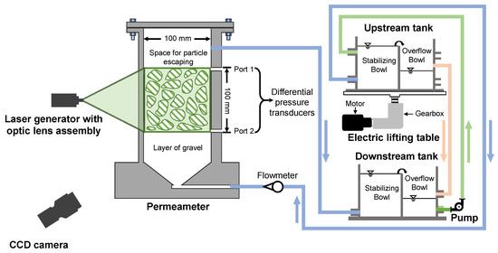
Figure 1.
Schematic diagram of the experimental system based on transparent soil and planar laser-induced fluorescence (PLIF) technique.
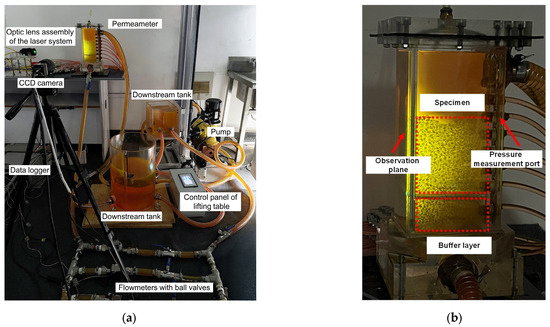
Figure 2.
Photographs of the experimental setup: (a) experimental system; (b) permeameter.
Two pressure measurement ports are located on the side wall of the permeameter at an interval of 100 mm to measure the hydraulic pressure drop using a differential pressure transducer with a capacity of 20 kPa and an accuracy of 0.04% full scale. Two oval gear flow meters, with measurement ranges of 100 to 1000 mL/min and 800 to 10,000 mL/min and an accuracy of 0.2% full scale, are connected in parallel between the outlet of the upstream fluid tank and the inlet of the permeameter to monitor liquid flow through the soil. Each flow meter is equipped with a ball valve, which can be adjusted during the experiment to ensure flow monitoring by an appropriate flowmeter.
The upstream and downstream fluid tanks are connected to the bottom and top of the permeameter, respectively, for upward seepage. The water head in both tanks is stabilized through overflow. The upstream tank is mounted on a lifting platform, allowing for adjustment of the head difference between the upstream and downstream tanks by altering the platform’s height, with a precision of 1 mm. The servo motor with a gearbox regulates the speed, height, number, and amplitude of the cyclic elevation of the upstream tank. An oil pump recirculates the mixed oil back to the upstream tank. The capacity of the pump is 4800 mL/min (0.8 cm/s for the permeameter with a cross-sectional area of 100 × 100 mm2 in this study), sufficient for the required seepage velocity in the following experiments.
Planar laser-induced fluorescence (PLIF) is employed to visualize the internal conditions within the soils [15]. A small amount of Nile Red dye is added to the mixed oil, causing it to emit orange-yellow light with a wavelength of 635 nm under laser illumination, while the fused silica sand remains non-luminescent. This allows for a clear distinction between the soil and fluid. The laser illumination is generated by a laser system comprising a laser generator, an optical lens assembly, and a fiber optic cable connecting them. The laser generator provides a point laser with an energy output of no less than 13 W. The optic lens assembly, located approximately 30 cm to the left of the permeameter, converts the point laser into a sheet laser with a thickness of 1 to 2 mm, illuminating the observation plane within the transparent soil specimen. The refractive index within the transparent soil cannot be completely uniform, leading to minor refraction that reduces the clarity of the observation plane as the soil thickness in front of it increases. Hence, the distance between the front wall of the permeameter and the observation plane illuminated by the laser is set as 6 dmax, which is determined by a parameter test, where dmax is the maximum particle diameter. A grayscale CCD camera with a 5-megapixel resolution is positioned in front of the permeameter to capture images of the observation plane.
2.2. Numerical Simulation Based on Coupled DEM–Darcy Method
To back-analyze the transparent soil tests, the coupled DEM–Darcy method is employed in PFC-3D to solve the hydro-mechanical behavior of the soil, as illustrated in the flowchart in Figure 3. The exchange of computational information between the DEM and Darcy modules is achieved using the FiPy solver [20] to process fluid-related data. FiPy, a Python-based library, is embedded within PFC-3D and facilitates fluid–particle coupling [21]. In each simulation loop, the contact forces among particles and their motion are first resolved using DEM. The classical Cundall linear model is applied to calculate the interparticle normal and shear contact forces [22].
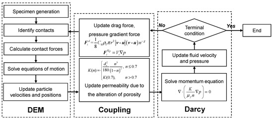
Figure 3.
Flowchart of coupled DEM-Darcy simulation.
The parameters are summarized in Table 2. The ratio of normal stiffness to particle radius (kn/r), the ratio of normal to tangential stiffness, and the interparticle friction coefficient are set to 100 MPa, 1, and 0.5, respectively, which are common values in previous studies [23,24,25]. Given the interparticle forces and the forces between particles and fluid from the previous loop, the motions of particles are updated by solving Newton’s second law.
Table 2.
Parameters in DEM simulations.
The seepage flow is solved using the generalized Darcy law, v = vseepage/n = −K/μn∇p, and the continuity equation, ∇v = 0. Here, v is the pore flow velocity; vseepage is the Darcy flow velocity; p is the average hydraulic pressure in a fluid grid; n is the porosity, calculated from particle position and size information [26]. The intrinsic permeability K is determined using the Kozeny–Carman model, expressed as de2n3/180(1 − n)2, where de is the average diameter of particles within a fluid grid. When n is larger than 0.7, K is taken as a fixed value, as suggested by references [27,28].
The forces between particles and fluid primarily include the pressure gradient force induced by the hydraulic pressure difference on one particle surface and the drag force induced by fluid viscosity, using the method proposed by Di Felice [29], as follows:
where Cd is the drag force coefficient, calculated as (0.63 + 4.8 (Rei)−0.5)2; u is the particle velocity vector; χ is the empirical coefficient to account for the local porosity, determined as 3.7 − 0.65exp(−0.5 × (1.5 − lgRei)2); and Rei is the particle Reynolds number, determined as 2ρfr|v − u|/μ. Some studies involving high-concentration suspensions have adopted the Di Felice drag force model and validated its applicability under such conditions [30,31]. The updated fluid–particle forces are then transferred back to the DEM for the next simulation loop. The time step for fluid and particle–fluid coupling is 10 times that of the DEM. After every 100 steps in DEM, the particle information and porosity are imported into the Darcy loop to solve the fluid governing equations.
The numerical model is depicted in Figure 4. Considering computational costs, the size of the numerical specimens is set to 50 × 50 × 50 mm3, which is half the experimental size in length. The specimen is enclosed by four rigid and impermeable side walls and one rigid and permeable bottom wall, while the top surface is free for particle escape. The numerical specimen is divided into cubic grids to determine the average seepage velocity tensor individually. The division of the fluid grid significantly affects calculation accuracy. As suggested by previous studies [24,25,32], the grid size should be 1 to 4 times larger than the average particle diameter, with at least five grids in each direction. Therefore, the cubic length of each grid is set to 10 mm, which is 6.62 to 7.58 times the average particle diameter in the simulation. To facilitate the application of boundary conditions, two additional rows of grids are added at the top and bottom of the particle model, respectively.
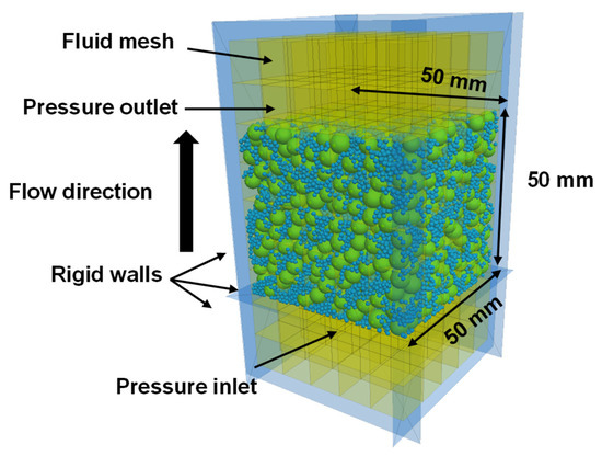
Figure 4.
Schematic diagram of coupled DEM–Darcy simulation model.
Although particle shape significantly affects suffusion behavior, simulations involving non-spherical particles are computationally intensive, and the realistic shape of particles is difficult to reconstruct. Therefore, spherical particles are used in this study, as in most previous studies. The radius expansion method [33] is employed to prepare the numerical specimens. Initially, the number of particles is calculated based on the target particle size distribution and void ratio. Particles smaller than the target size are randomly generated within a 50 × 50 × 50 mm3 space enclosed by six rigid walls, ensuring no interparticle contact. Subsequently, the radius of all soil particles gradually increases until reaching the target size, during which the unbalanced force is less than 0.01. After sampling, the top wall is removed, and gravity is applied. Once the unbalanced force is reduced to less than 1 × 10⁻⁵, a hydraulic gradient, iapp, is introduced by setting the hydraulic pressure at the outlet and inlet to 0 and iappH, respectively, where H is the height of the specimen (i.e., 50 mm). Each simulation with approximately 8400–20,000 soil particles requires approximately 40–180 h of computational time on a workstation equipped with a 16-core AMD5950X processor.
3. Experimental and Numerical Programs and Procedures
Three gap-graded soils are selected as shown in Figure 5. According to the internal stability prediction criteria by Kézdi [6] and Kenney and Lau [5], one gradation, composed of 20% fine particles (1–1.25 mm) and 80% coarse particles (4–5 mm), is deemed internally stable and is referred to as the “Stable” gradation. The other two gradations, containing 15% and 20% fine particles (1.25–1.43 mm) mixed with coarse particles (7–9 mm), are labeled as “Unstable-A” and “Unstable-B” gradations, respectively. The gap ratios of the “Stable”, “Unstable-A”, and “Unstable-B” gradations are 3.2, 4.9, and 4.9, respectively, as shown in Table 3.
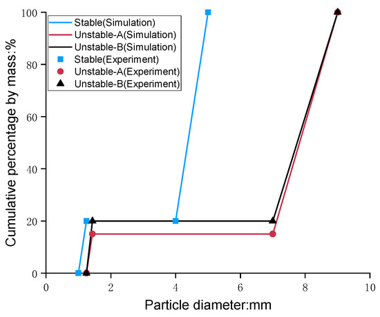
Figure 5.
Particle size distributions.
Table 3.
Internal stability prediction.
Three hydraulic loading paths are applied, as illustrated in Figure 6. In the first path of cyclic loading, the applied hydraulic gradient initially increases linearly from 0 to iav − Δi/2, then fluctuates cyclically with an amplitude of Δi, and finally increases linearly until failure. Here, iav is the average applied hydraulic gradient during cycling, and Δi is the cyclic applied hydraulic gradient amplitude, set at a constant value of 0.2 in this study. This path is simplified from the annual water level variations of a reservoir in the Three Gorges region of China, as reported by Yan [34] and Bao [35]. In this study, the cyclic number is 10, based on preliminary tests and simulations, which showed that the soil response to cyclic loading stabilized by the 10th cycle. The applied hydraulic gradient changes linearly rather than stepwise to facilitate hydraulic path setting during the cycling. The change rates of the applied hydraulic gradient during pre-cyclic, cyclic, and post-cyclic processes are a constant 0.015 min−1 in transparent soil tests, corresponding to a typical average change ratio of the hydraulic gradient in previous experiments under monotonic hydraulic loading [7,36,37]. To improve computational efficiency, the change rates of the hydraulic gradient in DEM simulations are set to 0.05 s−1, which is sufficient to maintain the simulation quasi-static, as indicated by an unbalanced force of no more than 0.01. Second, the monotonic linear loading serves as a reference to the cyclic hydraulic loading path, where the applied hydraulic gradient increases linearly from zero to failure at a rate consistent with that of the cyclic loading path. Third, the monotonic stepwise loading, commonly used in most previous studies [2,38,39,40,41], is employed to calibrate the effect of linear change on internal erosion behavior. In this path, the applied hydraulic gradient increases by 0.1 at each step, with an average change rate consistent with the linear change rate of the first two paths.
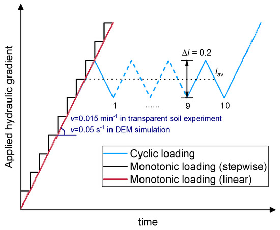
Figure 6.
Schematic diagram of applied hydraulic loading path.
Table 4 summarizes the experimental and simulation programs. Both monotonic hydraulic loading and cyclic hydraulic loading are applied in the experiments and simulations of each gradation. The mean hydraulic gradient during cycling, iav, is selected in the range of 0.6–0.9 icr-mono, where icr-mono is the critical hydraulic gradient during monotonic loading.
Table 4.
Experimental and numerical programs using transparent soil experiments and DEM simulations.
4. Macro-Behavior of Internal Erosion Subjected to Varying Loading Paths
4.1. Internal Erosion Behavior Under Monotonic Loading Paths
Figure 7 compares the seepage velocity–hydraulic gradient relationship curves between the monotonic linear and monotonic stepwise hydraulic loading paths in both transparent soil experiments and DEM simulations of Unstable-A. The seepage velocity increases with the applied hydraulic gradient, exhibiting three stages in both experiments and simulations. Initially, the relationship is linear, indicating limited particle migration under lower gradients. In this stage, the velocity–gradient relationship follows Darcy’s law, with the slope representing the permeability coefficient. The measured permeability coefficients under monotonic linear and stepwise hydraulic loading paths are 0.431 cm/s and 0.445 cm/s, respectively. The computed permeabilities are 0.545 cm/s and 0.553 cm/s, approximately 25.4% larger than the measured values, likely due to differences in particle shape between transparent soils and DEM simulations. In the second stage, the velocity increases nonlinearly with an increasing slope as the gradient rises further. This corresponds to the suffusion phenomenon [8,42,43], where finer particles migrate out of the specimen, increasing the void ratio and permeability. The inflection points of the velocity–gradient curves (i.e., the critical hydraulic gradient, icr) for monotonic linear and stepwise loading paths are 0.79 and 0.77 in transparent soils, and 0.87 and 0.90 in DEM simulations. The difference between the linear and stepwise loading paths is minimal, when the linear change rate of the former path is consistent with the average rate during the latter path, leading to the exclusive use of the monotonic linear path in other tests and simulations. The measured icr is 10% smaller than the computed value, possibly due to the higher drag forces on non-spherical fused quartz sands compared to spherical particles in DEM simulations. In the third stage, as the hydraulic gradient increases further, there is a noticeable deviation in the velocity–gradient curves between experiments and simulations. The experimental curves shift to the top left with a decreasing measured hydraulic gradient, while the numerical curves show a further increase in slope. Both phenomena indicate total heave failure. The different performances result from varying boundary conditions. In experiments, failure reduces the hydraulic resistance of the specimen, causing more hydraulic gradient to be applied to the tubes and less to the specimen, which is common in previous experiments [8,15,37]. In contrast, ideal boundary conditions in DEM simulations ensure the applied hydraulic gradient is fully borne by the specimen.
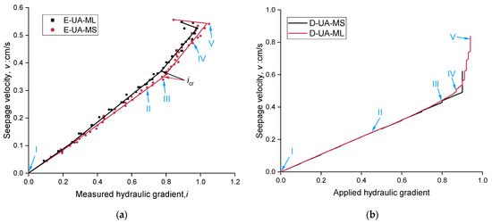
Figure 7.
Comparison between the measured and computed hydraulic velocity–gradient curve under monotonic loading (Unstable-A): (a) transparent soil experiment; (b) DEM simulation.
Figure 8 illustrates the evolution of internal sectional images under monotonic linear hydraulic loading in both experiments and simulations. In transparent soil experiments, no significant image change is observed initially. At i = 0.65, some fine particles begin to migrate from the voids among coarse particles. At i = 0.79, when icr is reached, local heave occurs at the top of the specimen, leading to an increase in permeability. At i = 0.95, some local clogging structures fail, with a small number of fine particles accumulating on the top surface of specimen. At i = 1.05, total heave failure occurs in the specimen, similar to phenomena observed by Hunter [15]. In the DEM simulation, the migration behavior of fine particles closely resembles experimental results and can be more clearly observed (the color of particles represents the height prior to hydraulic loading). At i = 0.45, fine particles begin to move upward. At i = 0.6, some fine particles clog in the upper area of the void enclosed by coarse particles. At i = 0.8, multiple clogging structures form internally, with fine particles concentrated at these structures, while migration channels form in other void areas, and fine particles on the top layer are eroded to the surface. At i = 0.87, when icr is reached, some clogging structures fail, and particles in the upper-middle part of the specimen are eroded to the surface, followed by total heave failure.
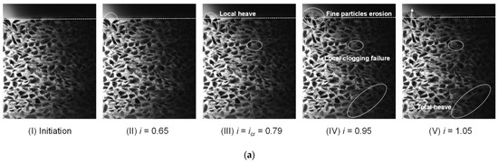
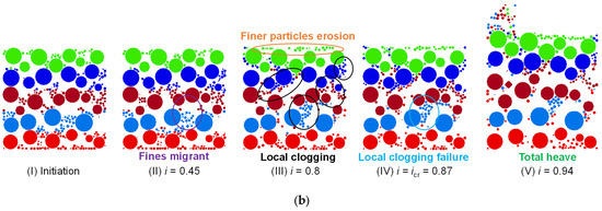
Figure 8.
Comparison between the observed and computed suffusion evolution at a cross-sectional plane subjected to monotonic linear hydraulic loading: (a) transparent soil experiment; (b) DEM simulation. Different colors represent particles located in different layers of the initial model.
4.2. Internal Erosion Behavior Under Cyclic Loading Paths
Figure 9 shows the velocity–gradient relationship curves under cyclic hydraulic loading. For the Stable soil, the linear velocity–gradient relationship remains almost unchanged during cyclic hydraulic loading. In contrast, the permeability of the Unstable soils increases progressively with each cycle, and the change in Unstable-A soil is more pronounced. This is because the void is larger for specimens with lower fine particle content, making fine particles more prone to erosion, thus leading to greater changes in permeability. The DEM simulation results indicate that the most noticeable permeability changes occur during the first three cycles, with diminishing changes as the number of cycles increases. The Unstable-A soil experiences a local upheaval failure during the cycles, causing a deflection in the velocity–gradient curve and a sudden increase in permeability. When the hydraulic gradient decreases, the detached fine particles gradually settle back, slightly reducing the permeability. The velocity–gradient curve then maintains a linear relationship, and the permeability remains constant for a period after the cyclic loading. In contrast, the Unstable-B soil specimen reaches the critical hydraulic gradient immediately after the cyclic loading.
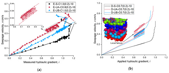
Figure 9.
Typical hydraulic velocity–gradient relationship with different particle size distributions under cyclic loading path: (a) transparent soil experiment; (b) DEM simulation.
Figure 10 illustrates the typical evolution of internal images from simulations of Unstable-A soils under cyclic loading. As the number of cycles increases, local clogging structures gradually break down, and fine particles are progressively eroded to the surface. During the first four cycles, there are significant failures of internal local clogging structures. In subsequent cycles, fine particles from these structures migrate within the voids and accumulate significantly at the top layer of the specimen. Based on the changes in permeability, it can be inferred that the alteration in specimen permeability is primarily due to the breakdown of clogging structures. The permeability changes caused by the loss of suspended fine particles are relatively minor in comparison.
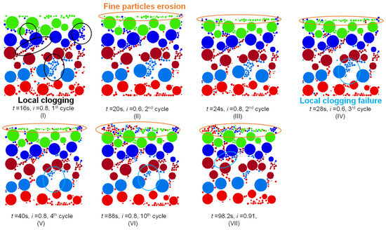
Figure 10.
Computed suffusion evolution at a cross-sectional plane subjected to cyclic hydraulic loading of DEM simulation (D-UA-C0.7(0.2)-10). Different colors represent particles located in different layers of the initial model.
4.3. Fines Migration During Cyclic Hydraulic Loading
In the study of hydraulic loading paths on internally unstable soils, changes in internal structure due to fine particle migration are the key cause of variations in permeability and critical hydraulic gradient. This paper proposes a modified grayscale threshold segmentation (MGTS) method to analyze fines migration based on grayscale observation plane images of transparent soils. The grayscale level of each pixel ranges from 0 (black) to 4095 (=212 − 1, white) for the 12-bit grayscale camera used in this study. In the images of the transparent soil observation plane, as shown in Figure 8a, there are significant grayscale differences among coarse particles, fine particles, and voids. The particles appear darker with lower grayscale levels, while the voids are lighter with higher grayscale levels. Coarse particles are darker than fine particles because the thickness of the laser plane is larger than the fine particle size. Therefore, coarse particles, fine particles, and voids can be identified based on the cumulative grayscale distribution of each image, as illustrated in Figure 11. The vertical axis, P, represents the percentage of pixels in the image with a grayscale value less than a certain level. P is an implicit function of grayscale G, determined by the geometric feature of the soil within the image area. During the process of suffusion, the geometric feature of the soil varies. Hence, G is a time-dependent function. Based on the volume division of the three regions in Figure 11, the proportion of fine particles, coarse particles, and void can be expressed as Equations (2)–(4):
where nt,a is the porosity in an area a at time t; VF, VC, and V are the volumes of fine particles, coarse particles, and void, respectively. The proportions of coarse particles and porosity can be similarly expressed.
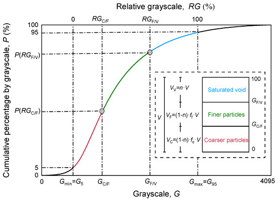
Figure 11.
Typical grayscale cumulative distribution curve of gap-graded soils.
Due to differences in lighting conditions across different regions of the image, the right side of the image has lower brightness. During processing, regions with relatively uniform brightness are selected for analysis. The selected area is divided into 8 × 10 subregions, each measuring 10 mm × 10 mm, as shown in Figure 12. Additionally, to avoid the influence of grayscale noise, relative grayscale (RG) is used to segment each image. The relative grayscale of area a at time t is expressed as Equation (5):
where Gmax and Gmin are the maximum and minimum grayscale values in an image, set to the 95% and 5% values, respectively. The corresponding grayscale values for the three parts are shown in Figure 11.
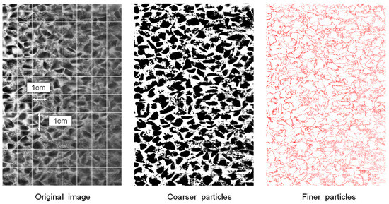
Figure 12.
Typical threshold segmentation result of transparent soil observation plane image.
The relative grayscale thresholds for distinguishing void, fine particles, and coarse particles can be expressed as Equations (6) and (7):
where P−1 is the inverse function of the initial cumulative distribution function of grayscale; nt0 is the initial porosity.
The proportion of fine particles, coarse particles, and void can finally be expressed as Equations (8)–(10):
where N is the number of subregions.
For the Unstable-A soil, the fine particle content and porosity are 15% and 0.4, respectively. The volume fractions of fine particles, coarse particles, and pores are assumed to correspond to the area fractions in the initial image, i.e., their grayscale cumulative proportions are 0.09, 0.51, and 0.4, respectively. Based on the grayscale cumulative proportions, the initial grayscale thresholds for coarse particles (GC/F) and fine particles (GF/V) are determined, and these two values are used as RGC/F and RGF/V. During the analysis, RGC/F and RGF/V remain constant, while variations in the image lead to changes in the grayscale cumulative distribution. This allows for the estimation of the volumetric changes in fine particles over time. Figure 12 shows the grayscale segmentation results for the Unstable-A specimen. The coarse particles are clearly segmented, while the segmented fine particles include some coarse particle outlines. This occurs due to the unavoidable grayscale gradient between coarse particles and voids, which can cross the grayscale threshold between coarse and fine particles, affecting the segmentation of fine particles. However, the outline portion is relatively small, so the result still reflects changes in fine particle content to some extent. The segmented images are then divided into five layers, and changes in fine particle proportion are calculated according to Equation (8).
Figure 13 compares the changes in fine particle content between layers determined by the MGTS method and in the DEM simulation. In the DEM simulation, when the applied hydraulic gradient reaches 0.4, fine particles in the lower two layers move upward. During cyclic loading, fine particles between the second and fourth layers gradually decrease, stabilizing after six cycles. This process corresponds to the gradual failure of the local clogging structures formed by fine particles. Under cyclic variations of the hydraulic gradient, some fine particles migrate vertically within the pore channels, causing the originally stable clogging structures to undergo repeated transitions between “dense” and “loose” states. With the increase in loading cycles, the force chain networks among fine particles are continuously reorganized, progressively weakening the local structural stability and eventually leading to the failure of the clogging structures. The fine particle content at the top layer slowly increases with fluctuation and then decreases rapidly after cyclic loading. As the critical hydraulic gradient is approached and heave failure occurs, the fine particle content in all layers decreases. Compared to the DEM simulation, the changes in fine particle content in the transparent soil experiment are more stable before reaching the critical hydraulic gradient. During cyclic loading, the fine particle content in the lower two layers changes slightly, while the upper three layers show fluctuations similar to the top layer in the DEM simulation. After reaching the critical hydraulic gradient, the fine particle content in all layers decreases, consistent with the DEM simulation results.
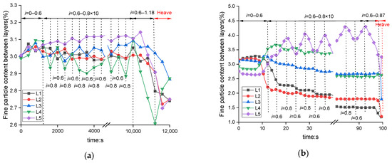
Figure 13.
Evolution of fine content between layers: (a) E-UA-C0.7(0.2)-10; (b) D-UA-C0.7(0.2)-10.
The differences between the two methods shown in Figure 13 can be attributed to two reasons. First, spherical particles in the DEM simulation are more likely to migrate compared to the non-spherical fused quartz sand, making fine particle migration more apparent in the simulation. Second, the MGTS method is based on 2D images from a fixed observation plane. Due to limitations in experimental techniques, only one fixed cross-sectional plane was selected during the test. However, the occurrence of suffusion is spatially random and may not take place within the observed plane, leading to an underestimation of fine particle migration. This reflects a limitation of the experimental approach. In future studies, the base of the permeameter could be redesigned to allow horizontal movement during testing, enabling the capture of cross-sectional images at different depths. These images can then be imported into specialized software to reconstruct a 3D model of the specimen, which would facilitate a more comprehensive understanding of fine particle migration and the development of preferential seepage paths.
4.4. Effects of Cyclic Hydraulic Loading on the Critical Hydraulic Gradient
Table 5 presents the values of icr and icr-cyc/icr-mono for each transparent soil experiment and DEM simulation, where icr-cyc is the critical hydraulic gradient after cyclic loading and icr-mono is the critical hydraulic gradient during monotonic loading. The maximum deviation in the critical hydraulic gradient (icr) between the transparent soil experiments and the DEM simulations under corresponding hydraulic conditions is 14.4%.
Table 5.
Critical hydraulic gradient: (a) transparent soil experiment; (b) DEM simulation.
Figure 14 illustrates the influence of the average hydraulic gradient iav on icr-cyc/icr-mono in both transparent soil experiments and DEM simulations. According to the results in Table 5 and Figure 14, different soil gradations show different icr-cyc/icr-mono in terms of iav. For Unstable-A, the icr-cyc is normally larger than icr-mono and increases with the increasing iav. In comparison with Unstable-B, the icr-cyc is always smaller than icr-mono and decreases with the increasing iav. This finding is consistent in both transparent soils and DEM simulations, although the deviations in simulations are slightly higher due to the different particle shapes, as mentioned. Additionally, Stable soil is less affected by cyclic loading, with icr-cyc/icr-mono close to 1.0. Figure 15 illustrates the influence of the hydraulic gradient amplitude and number of cycles on icr. As the amplitude of the cyclic hydraulic gradient increases, the icr of Unstable-B soil decreases. It can be observed that as the number of cycles increases, the cyclic hydraulic loading has a more pronounced effect on icr. Combined with Figure 9b, it is evident that the first three loading cycles have a greater impact on the permeability of the specimen.
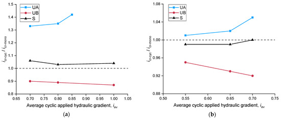
Figure 14.
Critical hydraulic gradient (icr-cyc) after varying average cyclically applied hydraulic gradient (iav): (a) transparent soil experiment; (b) DEM simulation.
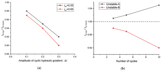
Figure 15.
Effects of the influencing factors on icr: (a) amplitude of cyclic hydraulic gradient (Unstable-B); (b) number of cycles.
5. Micro-Mechanical Analysis of Cyclic Effects on Internal Erosion
5.1. Evolution of Coordination Number
Figure 16 illustrates the evolution of the coordination number for Unstable-A and Unstable-B soils subjected to different loading paths in the DEM simulation. The coordination number, which represents the average number of contacts between particles in a specimen, is commonly used to assess soil structure stability [44]. Before the application of the hydraulic gradient, the coordination numbers for different gradations are around 3.6 to 3.7. When the applied hydraulic gradient (i) exceeds 0.2, the coordination number begins to decrease significantly due to particle erosion until i reaches around 0.5. As the hydraulic gradient i increases from 0.5 to 0.8, clogging structures gradually form, as shown in Figure 8b. The increase in interparticle contacts at clogging sites offsets the contact loss caused by fine particle erosion, resulting in a roughly constant coordination number during this phase. The coordination numbers for Unstable-A and Unstable-B remain constant at 2.6 and 3.0, respectively, due to the higher fine particle content in Unstable-B. Subsequently, during the first unloading phase (when i decreases from 0.8 to 0.6), the coordination numbers for both gradations return to approximately 3.1 to 3.3. After 10 cycles, the coordination numbers of both Unstable-A and Unstable-B increase due to the accumulation of fine particles at the top of the specimen.
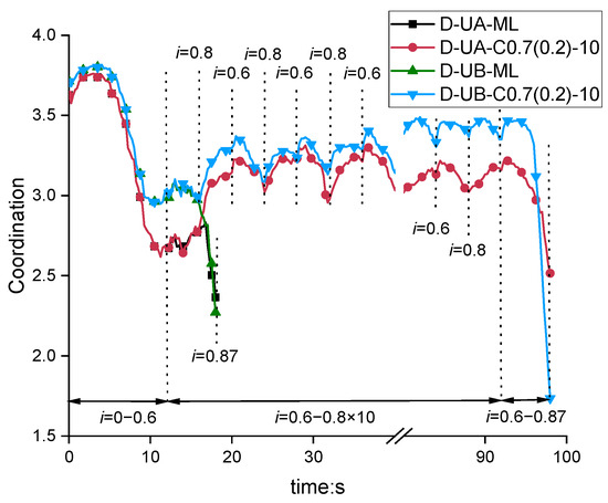
Figure 16.
Evolution of coordination number in DEM simulation.
5.2. Evolution of Force Chain
Figure 17 illustrates the evolution of the force chain structure in Unstable-A when iav is 0.7. As i increases from 0 to 0.6, the contact forces between both coarse and fine particles decrease, with many fine particles detaching from the skeleton and migrating within the voids. The contact forces between fine particles are smaller at the top and bottom of the sample and larger in the middle. When i reaches 0.8, a tight force chain network forms among the fine particles in the middle of the sample, increasing the contact forces between them. During subsequent cyclic loading, fine particles gradually accumulate at the top, reducing the force chain network among fine particles in the lower-middle part of the sample.
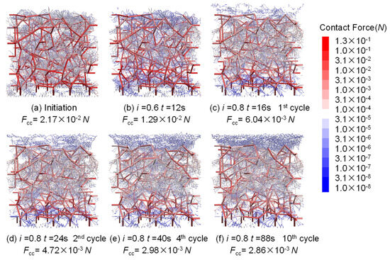
Figure 17.
Evolution of force chain (D-UA-C0.7(0.2)-10) in DEM simulation.
The magnitude of contact forces between coarse particles can indirectly reflect the structural stability of the soil. Figure 18 illustrates the average normal contact force between coarse particles (Fcc) in the DEM simulations. Fcc decreases as the hydraulic gradient increases from 0 to 0.8 in both Unstable-A and Unstable-B soils. During subsequent cyclic hydraulic loading, Fcc continues to decline with the number of cycles and eventually reaches a relatively stable value. The decrease in Fcc indicates a reduction in specimen stability during the cyclic hydraulic loading process.
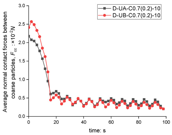
Figure 18.
Evolution of average normal contact force between coarse particles (Fcc) in DEM simulation.
Figure 19 shows the evolution of the average normal contact force between fine particles (Fff) in the DEM simulation. A higher Fff indicates that fine particles bear greater stress, making them less susceptible to erosion and leading to an increase in icr. To avoid the influence of fine particles transported to the top, Fff is calculated for those within the specimen height of 0–40 mm. The trends of Fff under cyclic loading differ between Unstable-A and Unstable-B soils. Compared to Fff under monotonic loading (Fff-mono), Fff under cyclic loading (Fff-cyc) in Unstable-A soil increases and continues to rise with increasing iav. During cyclic hydraulic loading, a considerable number of fine particles with low interparticle contact forces are eroded and transported away. The remaining fine particles experience higher stress within the soil structure, making them more resistant to erosion and thereby leading to an increase in icr. For Unstable-B soils, the amount of fine particle loss under cyclic hydraulic loading is relatively small. The local clogging structures within the voids are disrupted during cyclic hydraulic loading, and this disruption becomes more pronounced as iav increases. Most fine particles remain in a suspended state or exhibit low interparticle contact forces, making them more prone to erosion. As the cyclic hydraulic loading process continues, Fff-cyc gradually decreases and becomes lower than Fff-mono, leading to a reduction in icr.
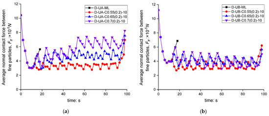
Figure 19.
Evolution of average normal contact force between fine particles (Fff) in DEM simulation: (a) Unstable-A; (b) Unstable-B.
6. Conclusions
This paper investigates the impact of cyclic hydraulic loading on the internal erosion processes of gap-graded soils by comparing findings from transparent soil experiments and coupled DEM–Darcy simulations. The study draws the following conclusions:
- (1)
- The internal cross-sectional images from both experiments and simulations exhibit a high degree of similarity. Typical suffusion phenomena, such as fine particle migration, clogging formation, and seepage channel development, are observed in both experimental and numerical settings. Cyclic hydraulic loading promotes a more gradual evolution of the soil’s microstructure. Unlike monotonic loading, cyclic loading causes local clogging structures to gradually break down, leading to fine particles migrating to the soil top surface.
- (2)
- A modified grayscale threshold segmentation (MGTS) method is developed to track fine particle migration across soil layers using images from transparent soil experiments. MGTS results show a slight decrease in fine content in the lower layers and a corresponding increase, with fluctuations, in the upper layers under cyclic loading. These trends are consistent with DEM simulation results.
- (3)
- Cyclic hydraulic loading affects the hydraulic behavior of internally unstable soils by breaking down clogging structures, which leads to an increase in soil permeability. Moreover, the critical hydraulic gradient (icr) for internally unstable soils changes after cycling. For Unstable-A soils (15% fines), the post-cyclic critical hydraulic gradient (icr-cyc) is higher than that under monotonic loading (icr-mono) and increases with the mean hydraulic gradient (iav). In contrast, for Unstable-B soils (20% fines), icr-cyc is lower than icr-mono and decreases with increasing iav.
- (4)
- DEM analysis provides a micro-mechanical explanation for the varying trend of iav. In Unstable-A soils, fine particles with lower average contact forces (Fff) are carried away, and remaining fines are subjected to higher Fff, increasing icr. In Unstable-B soils, local clogging structures are disrupted during cyclic hydraulic loading, causing a significant decrease in Fff among the remaining fine particles within the voids, leading to a decrease in icr.
This study evaluates the erosion resistance of gap-graded soils under monotonic and cyclic hydraulic loading paths, offering practical guidance for the selection of foundation materials in geotechnical engineering. The findings emphasize the significance of the loading path on both macro- and micro-scale hydraulic responses, which is particularly relevant for structures such as embankments and dams subjected to repeated water level fluctuations. In addition, the proposed MGTS method offers a new approach to image-based analysis in transparent soil experiments, enhancing the capability to quantitatively assess fine particle migration.
Author Contributions
Writing—original draft preparation, B.H. and X.Z.; writing—review and editing, X.Z. and C.G.; help and discussion, L.C.; funding acquisition, B.H. All authors have read and agreed to the published version of the manuscript.
Funding
The work presented in this article was supported by the Natural Science Foundation of Zhejiang Province (grant number LCZ19E080002) and the National Natural Science Foundation of China (Grant No. 51988101).
Data Availability Statement
Dataset available upon request from the authors.
Conflicts of Interest
The authors declare no conflicts of interest.
Abbreviations
The following abbreviations are used in this manuscript:
| CCD | Charge-coupled device |
| CFD | Computational fluid dynamics |
| CT | Computed tomography |
| DEM | Discrete element method |
| MGTS | Modified grayscale threshold segmentation |
| PFC-3D | Particle flow code—three-dimensional |
| PLIF | Planar laser-induced fluorescence |
| RI | Refractive index |
| 2D | Two-dimensional |
References
- Foster, M.; Fell, R.; Spannagle, M. The statistics of embankment dam failures and accidents. Can. Geotech. J. 2000, 37, 1000–1024. [Google Scholar] [CrossRef]
- Benamar, A.; Correia dos Santos, R.N.; Bennabi, A.; Karoui, T. Suffusion evaluation of coarse-graded soils from Rhine dikes. Acta Geotech. 2019, 14, 815–823. [Google Scholar] [CrossRef]
- Xiong, H.; Qiu, Y.; Liu, J.; Yin, Z.-Y.; Chen, X. Macro–microscopic mechanism of suffusion in calcareous sand under tidal fluctuations by coupled CFD-DEM. Comput. Geotech. 2023, 162, 105676. [Google Scholar] [CrossRef]
- Chen, C.; Zhang, L.M. Hydro-mechanical behaviour of soil experiencing seepage erosion under cyclic hydraulic gradient. Geotechnique 2023, 73, 115–127. [Google Scholar] [CrossRef]
- Kenney, T.C.; Lau, D. Internal stability of granular filters. Can. Geotech. J. 1985, 22, 215–225. [Google Scholar] [CrossRef]
- Kézdi, Á. Soil Physics: Selected Topics; Elsevier: Amsterdam, The Netherlands, 1979. [Google Scholar]
- Ke, L.; Takahashi, A. Experimental investigations on suffusion characteristics and its mechanical consequences on saturated cohesionless soil. Soils Found. 2014, 54, 713–730. [Google Scholar] [CrossRef]
- Skempton, A.W.; Brogan, J.M. Experiments on Piping in Sandy Gravels. Geotechnique 1994, 44, 449–460. [Google Scholar] [CrossRef]
- Shire, T.; O’Sullivan, C.; Hanley, K.J.; Fannin, R.J. Fabric and Effective Stress Distributionin Internally Unstable Soils. J. Geotech. Geoenviron. Eng. 2014, 140, 04014072. [Google Scholar] [CrossRef]
- Chang, D.S.; Zhang, L.M. Critical Hydraulic Gradients of Internal Erosion under Complex Stress States. J. Geotech. Geoenviron. Eng. 2013, 139, 1454–1467. [Google Scholar] [CrossRef]
- Luo, Y.L.; Luo, B.; Xiao, M. Effect of deviator stress on the initiation of suffusion. Acta Geotech. 2020, 15, 1607–1617. [Google Scholar] [CrossRef]
- Liang, Y.; Yeh, T.C.J.; Chen, Q.K.; Xu, W.; Dang, X.Y.; Hao, Y.H. Particle erosion in suffusion under isotropic and anisotropic stress states. Soils Found. 2019, 59, 1371–1384. [Google Scholar] [CrossRef]
- Xu, Z.D.; Zhang, L.M.; Kamali Zarch, M.; Wang, H.J. Experimental Study of Internal Erosion in Granular Soil Subject to Cyclic Hydraulic Gradient Reversal. J. Geotech. Geoenviron. Eng. 2022, 148, 04022014. [Google Scholar] [CrossRef]
- Cheng, Z.; Wang, J.F. Visualization of Failure and the Associated Grain-Scale Mechanical Behavior of Granular Soils under Shear using Synchrotron X-Ray Micro-Tomography. J. Vis. Exp. 2019, 152, e60322. [Google Scholar]
- Hunter, R.P.; Bowman, E.T. Visualisation of seepage-induced suffusion and suffosion within internally erodible granular media. Géotechnique 2018, 68, 918–930. [Google Scholar] [CrossRef]
- Iskander, M.; Bathurst, R.J.; Omidvar, M. Past, Present, and Future of Transparent Soils. Geotech. Test. J. 2015, 38, 557–573. [Google Scholar] [CrossRef]
- Nguyen, T.T.; Indraratna, B. A Coupled CFD–DEM Approach to Examine the Hydraulic Critical State of Soil under Increasing Hydraulic Gradient. Int. J. Geomech. 2020, 20, 04020138. [Google Scholar] [CrossRef]
- Hu, Z.; Zhang, Y.; Yang, Z. Suffusion-Induced Evolution of Mechanical and Microstructural Properties of Gap-Graded Soils Using CFD-DEM. J. Geotech. Geoenviron. Eng. 2020, 146, 04020024. [Google Scholar] [CrossRef]
- Zhang, P.; Mu, L.; Huang, M. A coupled CFD-DEM investigation into hydro-mechanical behaviour of gap-graded soil experiencing seepage erosion considering cyclic hydraulic loading. J. Hydrol. 2023, 624, 129908. [Google Scholar] [CrossRef]
- FiPy: A Finite Volume PDE Solver Using Python. Available online: http://www.ctcms.nist.gov/fipy (accessed on 7 April 2025).
- Yang, S.; Lv, Y.; He, Y.; Pang, M.; Ma, X. Mesoscale Numerical Analysis of Fiber-Reinforced Sand with Different Fiber Orientations Subjected to Seepage-Induced Erosion Based on DEM. Materials 2023, 16, 335. [Google Scholar] [CrossRef]
- Cundall, P.A.; Strack, O.D.L. A discrete numerical model for granular assemblies. Geotechnique 1979, 29, 47–65. [Google Scholar] [CrossRef]
- Wang, X.K.; Ling, D.S.; Tang, Y.; Hu, T.T.; Gao, Z.C.; Chen, Y.M. Hydraulic heave in granular soils under hypergravity conditions. Powder Technol. 2024, 440, 119764. [Google Scholar] [CrossRef]
- Hu, Z.; Zhang, Y.; Yang, Z. Suffusion-induced deformation and microstructural change of granular soils: A coupled CFD–DEM study. Acta Geotech. 2019, 14, 795–814. [Google Scholar] [CrossRef]
- Tao, H.; Tao, J. Quantitative analysis of piping erosion micro-mechanisms with coupled CFD and DEM method. Acta Geotech. 2017, 12, 573–592. [Google Scholar] [CrossRef]
- Itasca Consulting Group, Inc. PFC—Particle Flow Code, Ver. 5.0; Itasca: Minneapolis, MN, USA, 2014.
- Nguyen, T.T.; Indraratna, B. The role of particle shape on hydraulic conductivity of granular soils captured through Kozeny-Carman approach. Geotech. Lett. 2020, 10, 398–403. [Google Scholar] [CrossRef]
- Carrier, W.D. Goodbye, Hazen; Hello, Kozeny-Carman. J. Geotech. Geoenvironmental Eng. 2003, 129, 1054–1056. [Google Scholar] [CrossRef]
- Difelice, R. The Voidage Function for Fluid Particle Interaction Systems. Int. J. Multiph. Flow 1994, 20, 153–159. [Google Scholar] [CrossRef]
- Qian, J.-G.; Zhou, C.; Yin, Z.-Y.; Li, W.-Y. Investigating the effect of particle angularity on suffusion of gap-graded soil using coupled CFD-DEM. Comput. Geotech. 2021, 139, 104383. [Google Scholar] [CrossRef]
- Cheng, K.; Wang, Y.; Yang, Q. A semi-resolved CFD-DEM model for seepage-induced fine particle migration in gap-graded soils. Comput. Geotech. 2018, 100, 30–51. [Google Scholar] [CrossRef]
- Wang, X.; Huang, B.; Tang, Y.; Hu, T.; Ling, D. Microscopic mechanism and analytical modeling of seepage-induced erosion in bimodal soils. Comput. Geotech. 2022, 141, 104527. [Google Scholar] [CrossRef]
- Dong, Q.; Wang, Y.; Feng, D. An algorithm to generate dense and stable particle assemblies for 2D DEM simulation. Eng. Anal. Bound. Elem. 2020, 114, 127–135. [Google Scholar] [CrossRef]
- Yan, L.; Xu, W.; Wang, H.; Wang, R.; Meng, Q.; Yu, J.; Xie, W.-C. Drainage controls on the Donglingxing landslide (China) induced by rainfall and fluctuation in reservoir water levels. Landslides 2019, 16, 1583–1593. [Google Scholar] [CrossRef]
- Bao, Y.; Gao, P.; He, X. The water-level fluctuation zone of Three Gorges Reservoir—Aunique geomorphological unit. Earth-Sci. Rev. 2015, 150, 14–24. [Google Scholar] [CrossRef]
- Radjai, F.; Nguyen, C.D.; Benahmed, N.; Philippe, P.; Diaz Gonzalez, E.V.; Nezamabadi, S.; Luding, S.; Delenne, J.Y. Experimental study of erosion by suffusion at the micro-macro scale. EPJ Web Conf. 2017, 140, 09024. [Google Scholar]
- Yang, K.-H.; Wang, J.-Y. Experiment and statistical assessment on piping failures in soils with different gradations. Mar. Georesour. Geotechnol. 2016, 35, 512–527. [Google Scholar] [CrossRef]
- Hu, Z.; Yang, Z.X.; Zhang, Y.D. CFD-DEM modeling of suffusion effect on undrained behavior of internally unstable soils. Comput. Geotech. 2020, 126, 103692. [Google Scholar] [CrossRef]
- Gelet, R.; Marot, D. Internal erosion by suffusion on cohesionless gap-graded soils: Model and sensibility analysis. Geomech. Energy Environ. 2022, 31, 100313. [Google Scholar] [CrossRef]
- Cheng, K.; Zhang, C.; Peng, K.; Liu, H.; Ahmad, M. Un-resolved CFD-DEM method: An insight into its limitations in the modelling of suffusion in gap-graded soils. Powder Technol. 2021, 381, 520–538. [Google Scholar] [CrossRef]
- Chen, R.; Liu, L.; Li, Z.; Deng, G.; Zhang, Y.; Zhang, Y. A novel vertical stress-controlled apparatus for studying suffusion along horizontal seepage through soils. Acta Geotech. 2021, 16, 2217–2230. [Google Scholar] [CrossRef]
- Kodieh, A.; Gelet, R.; Marot, D.; Fino, A.Z. A study of suffusion kinetics inspired from experimental data: Comparison of three different approaches. Acta Geotech. 2020, 16, 347–365. [Google Scholar] [CrossRef]
- Zhong, C.; Le, V.T.; Bendahmane, F.; Marot, D.; Yin, Z.-Y. Investigation of Spatial Scale Effects on Suffusion Susceptibility. J. Geotech. Geoenviron. Eng. 2018, 144, 04018067. [Google Scholar] [CrossRef]
- Shire, T.; O’Sullivan, C. Micromechanical assessment of an internal stability criterion. Acta Geotech. 2013, 8, 81–90. [Google Scholar] [CrossRef]
Disclaimer/Publisher’s Note: The statements, opinions and data contained in all publications are solely those of the individual author(s) and contributor(s) and not of MDPI and/or the editor(s). MDPI and/or the editor(s) disclaim responsibility for any injury to people or property resulting from any ideas, methods, instructions or products referred to in the content. |
© 2025 by the authors. Licensee MDPI, Basel, Switzerland. This article is an open access article distributed under the terms and conditions of the Creative Commons Attribution (CC BY) license (https://creativecommons.org/licenses/by/4.0/).