Integrated Hydrologic–Hydraulic Modeling Framework for Flood Risk Assessment of Rural Bridge Infrastructure in Northwestern Pakistan

Abstract

This study presents a flood risk assessment of five rural bridges along the monsoon-prone Khar–Mohmand Gat corridor in Northwestern Pakistan using an integrated hydrologic and hydraulic modeling framework. Hydrologic simulations for 50- and 100-year design storms were performed using the Hydrologic Engineering Center’s Hydrologic Modeling System (HEC-HMS), with watershed delineation conducted via Geographic Information Systems (GIS). Calibration was based on regional rainfall data from the Peshawar station using a Soil Conservation Service Curve Number (SCS-CN) of 86 and time of concentration calculated using Kirpich’s method. The resulting hydrographs were used in two-dimensional hydraulic simulations using the Hydrologic Engineering Center’s River Analysis System (HEC-RAS) to evaluate water surface elevations, flow velocities, and Froude numbers at each bridge site. The findings reveal that all bridges can convey peak flows without overtopping under current climatic conditions. However, Bridges 3 to 5 experience near-critical to supercritical flow conditions, with velocities ranging from 3.43 to 4.75 m/s and Froude numbers between 0.92 and 1.04, indicating high vulnerability to local scour. Bridge 2 shows moderate risk, while Bridge 1 faces the least hydraulic stress. The applied modeling framework effectively identifies structures requiring priority intervention and demonstrates a practical methodology for assessing flood risk in ungauged, data-scarce, and semi-arid regions.

1. Introduction

Rural transportation infrastructure, particularly bridges, forms the critical backbone of socio-economic activity in developing regions, enabling access to markets, healthcare, education, and emergency services [1]. However, this infrastructure is increasingly vulnerable to escalating climate impacts, particularly flooding, the most frequent and devastating natural disaster globally [2]. The failure of a single rural bridge can sever essential connections, crippling local economies and endangering lives, especially in remote areas with limited alternative routes [3]. Consequently, robust flood risk assessment (FRA) is paramount for ensuring the resilience, safety, and longevity of these vital assets.

Northwestern Pakistan, encompassing regions like Khyber Pakhtunkhwa (KP), exhibits extreme vulnerability to flooding. Characterized by complex topography, a semi-arid climate, intense monsoon rainfall, and rapidly melting glaciers in the Hindu Kush-Himalayan region, the area is prone to frequent and often catastrophic flood events [4,5]. The devastating floods of 2010, 2012, and most recently 2022, underscored the region’s susceptibility, causing widespread infrastructure damage, including numerous bridge failures, and highlighting the inadequacy of existing design and mitigation strategies [6,7]. Utilizing static design storms, such as the 50-year and 100-year return period events, remains a cornerstone of engineering practice for infrastructure design and FRA. These benchmarks provide standardized, albeit simplified, estimates of extreme hydrological loading necessary for evaluating structural adequacy and identifying vulnerabilities under plausible worst-case scenarios [8]. Assessing infrastructure against these events is crucial for prioritizing retrofitting investments in resource-constrained environments like rural Pakistan. Static return-period designs increasingly underestimate flood hazards under climate non-stationarity [9], necessitating adaptive frameworks for rural infrastructure.

Accurately simulating flood hazards in data-scarce, semi-arid regions like Northwestern Pakistan presents significant challenges where direct streamflow observations are unavailable. As established in the hydrological literature [10], integrated hydrologic-hydraulic modeling frameworks provide a scientifically robust alternative, leveraging synthetic approaches to overcome observational data limitations. Hydrologic models, such as the Hydrologic Engineering Center’s Hydrologic Modeling System (HEC-HMS), simulate the transformation of rainfall into runoff, generating inflow hydrographs for rivers and streams [11]. These hydrographs then serve as critical input for hydraulic models, like the Hydrologic Engineering Center’s River Analysis System (HEC-RAS), which simulate water flow through river channels and floodplains, predicting water surface elevations, flow velocities, and inundation extents around structures like bridges [12]. Integrating Geographic Information Systems (GIS) facilitates essential tasks like watershed delineation, parameter estimation, and flood hazard visualization. This combined approach (HEC-HMS+HEC-RAS + GIS) is particularly valuable in ungauged or poorly gauged basins, allowing for a physically based assessment of flood risk where direct observational data are limited [13,14].

2. Research Gap

Despite the critical vulnerability of rural bridges in Northwestern Pakistan to monsoon flooding, site-specific FRA integrating hydrologic–hydraulic modeling for scour risk evaluation remains limited. Few studies leverage advanced frameworks (HEC-HMS/HEC-RAS) to prioritize retrofitting of minor bridges in ungauged semi-arid basins under 50-/100-year storms, particularly linking hydraulic outputs (velocity and Froude number) to localized failure mechanisms.

This study addresses this gap by assessing five rural bridges in the Khar–Mohmand Gat corridor using integrated modeling under design storms.

3. Literature Review

3.1. Recent Advances in Flood Risk Assessment for Bridges

Flood risk assessment for bridges has evolved significantly, moving beyond simple peak flow estimation toward integrated frameworks considering hydrologic processes, detailed hydraulic behavior, structural vulnerability, and socio-economic consequences [15]. Recent research emphasizes the importance of quantifying multiple failure modes, including overtopping, scour at piers and abutments, deck uplift, and structural collapse due to hydrodynamic forces [16]. Studies increasingly utilize high-resolution topographic data (e.g., LiDAR) and advanced 2D hydraulic modeling within HEC-RAS or similar software (e.g., TELEMAC-2D, MIKE FLOOD, version HEC-RAS 6.6) to capture complex flow patterns and velocity distributions around bridge structures, which are critical for scour prediction [17,18]. The concept of “resilience” is also gaining traction, focusing not just on preventing failure, but also on minimizing disruption and enabling rapid recovery [19]. Recent reviews confirm that AI hybrid models achieve >90% accuracy in scour depth prediction [20], though data requirements limit their use in ungauged basins like ours.

3.2. Flood Impacts on Infrastructure in Pakistan and Comparable Regions

Research specific to flood risks on infrastructure in Pakistan has intensified following major events. Studies highlight widespread damage to roads and bridges during the 2010, 2012, and 2022 floods, often attributing failures to inadequate design standards, poor construction, lack of maintenance, and underestimation of current and future flood magnitudes [21,22]. Research in the Swat and Kabul River basins, hydrologically relevant to Northwestern Pakistan, has employed modeling to reconstruct flood events and assess impacts, confirming the severe vulnerability of infrastructure [3,4]. Similar challenges are documented in other semi-arid, monsoon-influenced, data-scarce regions globally. Studies in India (e.g., Himachal Pradesh, Uttarakhand), Ethiopia, and Nepal demonstrate comparable issues of intense rainfall, flash floods, sediment transport, and bridge vulnerabilities, often employing similar integrated modeling approaches tailored to limited data availability [13,14,23].

3.3. Application of HEC-HMS and HEC-RAS in Flood Modeling

The HEC software suite (HMS 4.11 and RAS 6.6) remains a globally prevalent toolset for integrated FRA due to its robustness, continuous development, free availability, and extensive user community support. Recent applications demonstrate their effectiveness in diverse settings:

• HEC-HMS: Widely used for rainfall runoff modeling in ungauged basins, employing methods like SCS-CN, Clark’s Unit Hydrograph, and kinematic wave routing. Studies successfully apply it for design flood estimation and climate change impact assessment in regions like Ethiopia, India, and Iran, validating its utility in data-scarce environments [13,23,24].
• HEC-RAS: The adoption of 2D modeling capabilities within HEC-RAS (versions 5.0 and later) has revolutionized detailed flood inundation and bridge hydraulics simulation. Recent research extensively uses HEC-RAS 2D for high-fidelity modeling of flow around bridges, predicting scour potential, evaluating overtopping risks, and mapping flood hazards with greater accuracy than traditional 1D approaches [17,18,25]. Its integration with GIS for pre- and post-processing is standard practice [12].

3.4. Impact of Climate Change on Hydrologic and Hydraulic Modeling

Climate change is profoundly altering the hydrological cycle, challenging traditional FRA methodologies. Observed and projected trends include increased rainfall intensity, shifting storm tracks, changing snowmelt patterns, and more frequent extreme events, rendering historical data less reliable for predicting future risks [26,27]. This has significant implications for modeling:

• Design Storm Obsolescence: Static design storms (e.g., 100-year) based solely on historical records may underestimate future flood magnitudes. Researchers increasingly advocate for Non-Stationary Frequency Analysis (NSFA) or using climate projections to adjust design storm intensities and durations [8,28];
• Model Parameterization: Changing land use/land cover and rainfall patterns may alter watershed response characteristics (e.g., CN values, runoff coefficients), requiring dynamic model parameterization or scenario-based analysis [14];
• Increased Scour Risk: Higher flow velocities and altered sediment transport regimes associated with more intense floods can exacerbate scour, a primary bridge failure mechanism, necessitating more rigorous scour analysis in hydraulic models [29]. Recent experimental studies demonstrate collar-based systems effectively reduce scour depth by 40–70% at abutments [30];
• Uncertainty Quantification: Incorporating climate projections introduces significant uncertainty into FRA. The recent literature emphasizes the need for ensemble modeling, sensitivity analysis, and transparent communication of uncertainties in flood risk estimates [15,28].

4. Study Area and Data

Location and Catchment: The study corridor is a mountainous region in northwestern Pakistan, along the road from Khar to Mohmand Gat. Five bridge sites (denoted Bridge 1 through Bridge 5) are located on tributary streams that drain semi-arid hills. The watersheds of these streams were delineated using topographic maps and a 30 m resolution digital elevation model (DEM). The coordinate reference system (WGS 84) and datum used for the analysis were also included to ensure reproducibility. The catchment areas and key geomorphic parameters for each bridge site are summarized in

Table 1. Watershed characteristics of the five bridge catchments along the Khar–Mohmand Gat Road.

No	Description	Catchment Area	Length of Longest Stream (m)	Height Difference	Slope (m/m)
		(Sq Km)		“H” (m)
1	Bridge 1	60.035	19,065.016	958	0.0502
2	Bridge 2	6.435	6000	325	0.0541
3	Bridge 3	11.873	6300	269	0.0426
4	Bridge 4	108.307	24,243.48	1248	0.0515
5	Bridge 5	8.072	4013.91	96	0.0239

. Bridge 4 drains the largest basin (~108.3 km²), while Bridge 2 has the smallest catchment (~6.4 km²). The longest flow path lengths range from about 4 km to 24 km, and catchment slopes are on the order of 0.024–0.054 (dimensionless). These characteristics give an initial indication of the expected runoff response: larger and longer catchments (like Bridge 4) would generate greater flood volumes and somewhat delayed peaks, whereas smaller steeper basins (like Bridge 2) would respond more quickly to intense rainfall, but with lesser total discharge.

Figure 1 shows the location map for the bridge sites. The main purpose of the hydrological study is to estimate design flood parameters for each stream crossing along the road alignment. These estimates form the basis for carrying out hydraulic design checks for cross-drainage works (bridges). Table 1 presents the watershed characteristics for the five bridge sites:

5. Methodology

• Hydrological Analysis

• Hydro-Meteorological Data

Stream flow Data: There are no stream flow gauging station and data available for the streams at the proposed bridge. In the light of monitoring carried out during field surveys, the river flow is assessed to be seasonal generated mainly by rainfall.

Rainfall Data: There is no rainfall gauging station within the catchment area. Therefore, the data of the rain gauge station of Peshawar (located at the periphery of the catchment) were used for hydrological analysis.

Annual and monthly Isohyetal maps were prepared for the years of record, using climate stations operated and maintained by the Pakistan Meteorological Department (PMD). The areal adjustment factors of rainfall were calculated from rainfall data at Peshawar station. The mean annual rainfall at Peshawar is 382 mm (

Table 2. Monthly rainfall data at Peshawar (1970–2015) in millimeters.

Year	1	2	3	4	5	6	7	8	9	10	11	12
	Jan	Feb	Mar	Apr	May	Jun	Jul	Aug	Sep	Oct	Nov	Dec	MAX
1970	13.05	25.56	12.78	15.57	0.27	5.76	31.05	49.14	45.72	0.00	0.00	3.24	49.14
1971	1.62	22.14	20.16	76.14	5.04	5.49	15.30	20.34	27.45	5.22	0.00	5.49	76.14
1972	16.65	40.50	17.19	38.61	9.63	8.91	7.11	4.59	9.36	0.72	8.46	13.68	40.50
1973	3.24	23.76	41.13	6.21	31.77	0.00	9.81	17.37	35.46	2.70	0.00	4.59	41.13
1974	4.32	15.39	4.32	17.46	2.25	0.00	11.52	11.34	9.00	0.00	0.00	7.11	17.46
1975	0.36	15.30	26.19	18.90	20.25	2.70	47.97	44.01	1.80	0.00	0.00	4.77	47.97
1976	8.73	21.33	36.72	32.94	2.61	11.43	9.00	91.80	9.00	6.30	0.00	0.90	91.80
1977	22.23	10.62	0.00	44.10	7.74	0.00	102.15	4.95	26.55	2.16	15.21	5.40	102.15
1978	10.44	11.70	61.47	6.30	0.90	7.65	15.48	19.98	7.56	2.70	15.93	0.00	61.47
1979	48.96	28.26	20.88	8.28	28.80	8.10	9.90	23.40	0.10	0.00	12.87	0.54	48.96
1980	13.50	40.50	22.68	6.48	8.10	18.27	41.49	33.75	4.50	3.60	5.40	1.80	41.49
1981	9.54	11.25	50.40	19.08	18.27	0.90	10.80	30.15	0.01	4.86	0.01	0.01	50.40
1982	11.70	6.21	22.05	6.93	2.25	1.26	1.80	30.24	0.00	0.90	36.90	10.89	36.90
1983	12.24	16.92	24.39	46.35	18.90	11.97	29.70	76.23	13.95	8.28	9.00	1.44	76.23
1984	3.51	9.90	12.42	26.19	3.15	3.60	47.70	78.12	8.55	0.00	8.10	2.07	78.12
1985	20.79	5.04	16.65	13.05	6.75	0.01	13.50	55.80	2.70	0.90	7.20	28.35	55.80
1986	13.77	33.48	27.00	6.30	7.20	14.40	18.00	32.40	13.95	0.01	42.75	14.85	42.75
1987	0.00	35.64	47.16	4.05	15.21	9.00	3.24	0.00	4.23	27.90	0.00	2.70	47.16
1988	25.29	8.10	28.35	7.38	3.60	2.52	10.62	39.87	4.95	7.20	0.00	19.53	39.87
1989	27.00	6.30	8.73	8.10	7.38	0.45	31.50	14.40	8.10	8.10	2.70	13.50	31.50
1990	28.08	18.27	18.00	9.90	8.10	2.16	6.66	49.50	28.53	29.88	4.05	20.16	49.50
1991	5.58	15.12	55.80	25.20	39.60	0.90	9.90	15.30	2.70	1.80	2.70	2.70	55.80
1992	38.79	31.50	24.30	24.30	18.00	1.80	3.60	50.40	9.00	12.60	0.00	29.70	50.40
1993	10.80	12.15	60.30	14.40	6.30	23.76	18.00	0.00	36.00	9.00	4.50	0.00	60.30
1994	13.50	45.90	16.20	38.70	10.80	5.40	37.80	18.00	39.60	31.50	0.90	18.90	45.90
1995	0.00	15.30	40.32	32.22	10.80	0.90	49.50	30.60	40.50	7.20	11.70	1.80	49.50
1996	16.20	25.20	16.20	24.30	5.40	9.00	15.30	54.00	23.40	127.80	36.90	0.00	127.80
1997	10.80	11.70	8.10	34.20	9.00	27.00	14.40	9.90	9.00	24.30	1.80	19.35	34.20
1998	27.00	34.20	27.00	35.10	11.70	21.15	25.20	42.30	10.80	4.05	0.00	0.00	42.30
1999	27.00	9.90	20.70	0.00	3.15	43.20	18.90	7.20	9.90	0.90	18.00	0.00	43.20
2000	29.70	24.75	18.00	2.70	8.10	7.20	4.50	10.80	10.80	4.50	0.00	13.50	29.70
2001	0.00	0.90	24.30	24.30	16.20	18.90	18.00	11.70	16.20	0.00	8.10	0.00	24.30
2002	0.90	26.10	26.10	5.40	5.40	27.00	0.00	0.00	18.00	1.80	5.40	26.10	27.00
2003	29.70	49.50	22.50	49.50	13.50	9.00	63.90	40.50	58.50	62.10	30.60	13.50	63.90
2004	37.80	61.20	0.00	23.40	0.00	0.00	4.50	28.80	24.30	22.50	13.50	13.50	61.20
2005	64.80	25.20	32.40	21.60	16.20	0.00	13.50	20.70	22.50	16.20	162.00	0.00	162.00
2006	23.85	11.70	14.40	6.30	5.40	9.90	45.90	9.90	11.70	16.20	15.30	50.40	50.40
2007	0.00	75.60	41.40	18.00	7.20	55.80	45.00	18.00	27.00	0.00	10.80	0.90	75.60
2008	17.64	7.65	7.74	43.20	2.43	8.64	30.60	53.10	10.80	0.00	1.08	6.84	53.10
2009	11.70	17.10	14.13	24.30	34.20	0.90	11.70	32.40	12.60	0.00	12.60	0.54	34.20
2010	17.64	19.98	4.50	4.32	6.30	16.02	183.60	58.50	3.96	0.00	0.00	8.28	183.60
2011	0.54	28.98	4.50	15.66	7.20	2.52	11.70	65.70	19.80	12.60	8.10	0.00	65.70
2012	27.00	11.07	4.50	21.60	10.80	3.60	0.00	53.10	35.10	8.10	1.17	32.22	53.10
2013	2.70	72.00	36.00	41.22	9.90	9.00	14.40	9.00	2.70	8.64	14.40	0.90	72.00
2014	4.68	14.40	28.80	19.80	5.40	23.04	17.37	40.50	12.60	17.10	0.90	0.00	40.50
2015	24.57	25.47	42.30	53.10	18.00	0.00	34.20	48.60	42.30	15.30	18.00	5.40	53.10
Mean	16.04	23.45	24.11	22.20	10.64	9.55	25.34	31.66	16.77	11.21	11.89	8.82	58.37

).

Table 2 presents the monthly rainfall totals at Peshawar for each year of record (1970–2015). The final column (“MAX”) is the maximum monthly rainfall observed in that year.

Areal Reduction Factor. Rainfall over a large area such as a catchment is related to point rainfall by using an “Areal Reduction Factor” (ARF). See Figure 2.

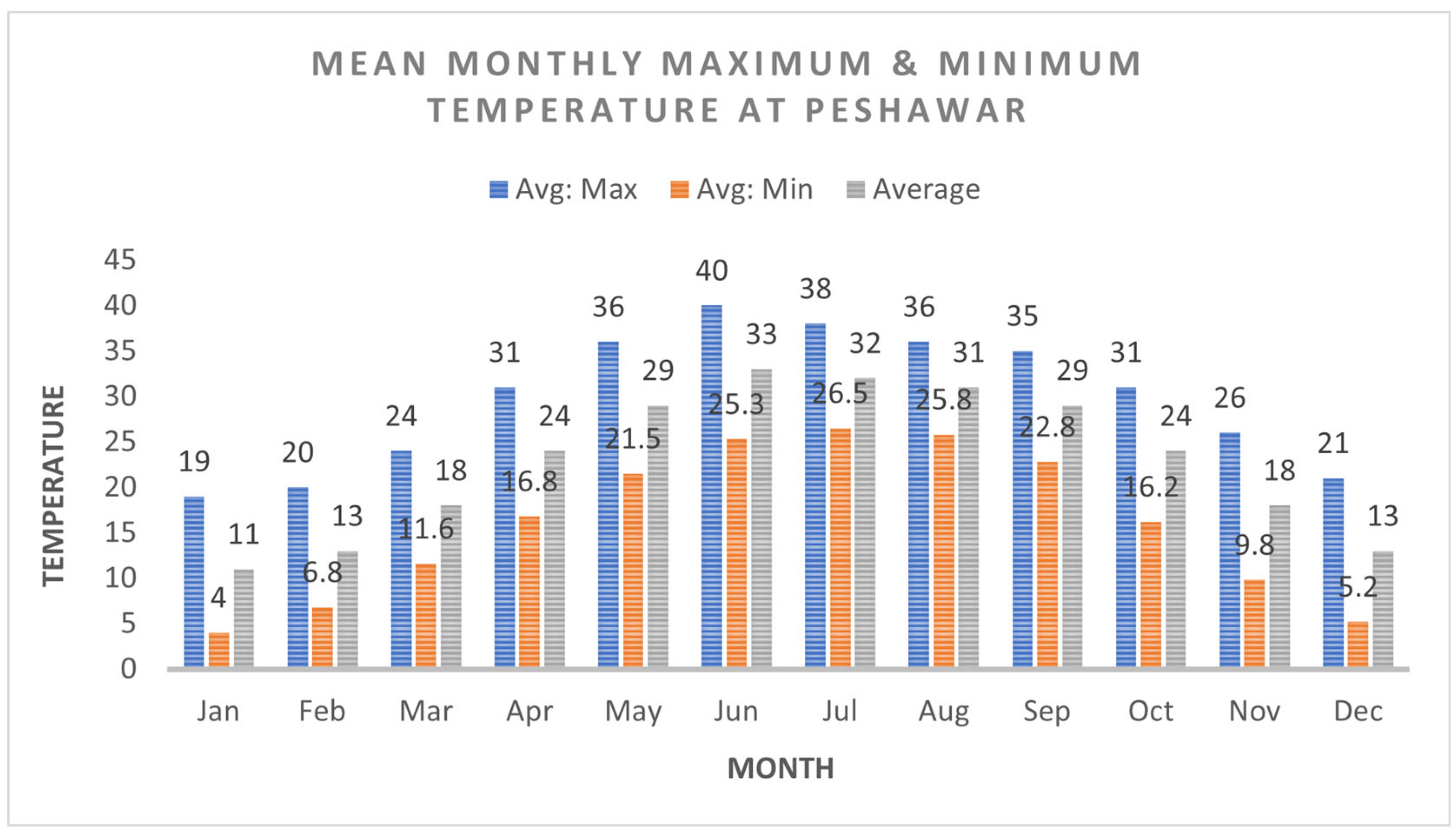
Temperature Data: The monthly temperature record of the meteorological station at Peshawar for the period 1974–2012 was acquired.

Table 3. Mean monthly minimum and maximum temperature at Peshawar (°C).

Month	Jan	Feb	Mar	Apr	May	Jun	Jul	Aug	Sep	Oct	Nov	Dec
Avg: Max	19.0	20.0	24.0	31.0	36.0	40.0	38.0	36.0	35.0	31.0	26.0	21.0
Avg: Min	4.0	6.8	11.6	16.8	21.5	25.3	26.5	25.8	22.8	16.2	9.8	5.2
Average	11.0	13.0	18.0	24.0	29.0	33.0	32.0	31.0	29.0	24.0	18.0	13.0

Note: Source: Pakistan Meteorological Department, Peshawar.

provides the monthly maximum and minimum values of temperature, which are graphically presented in Figure 3. The average temperature varies from 11.0 °C to 33.0 °C during the calendar year. The data indicate that the average maximum temperature varies from 20.0 °C to 40.0 °C, while the minimum average temperature ranges from 4.0 °C to 27.0 °C during the year.

Evaporation Data: Monthly pan evaporation data from Peshawar station for the period of 1985–2004 were obtained from the Pakistan Forest Institute, Peshawar. The mean annual pan evaporation for Peshawar is 1295.40 mm (51 inch). The monthly pan evaporation data for Peshawar Station are provided in

Table 4. Mean monthly pan evaporation at Peshawar (1985–2004).

Year/Month	Jan	Feb	Mar	Apr	May	Jun	Jul	Aug	Sep	Oct	Nov	Dec	Total
Average	53	60	94	113	132	218	184	131	119	102	48	36	1290
Max	254	127	152	152	203	432	203	178	178	178	76	102	2235
Min	25	25	76	76	76	152	127	102	76	76	25	25	861

Note: Source: Pakistan Forest Institute, Peshawar.

and Figure 4.

Overall, the climate of the study area is characterized by low to moderate annual rainfall, but with a pronounced summer monsoon that can produce extreme precipitation events. High temperatures and evaporation in the pre-monsoon months can lead to dry antecedent conditions, but once the monsoon arrives, intense rainfall on potentially dry soils can result in rapid runoff (flash floods). These factors were taken into account when establishing the parameters for the hydrologic model.

• Flood Studies

Design Flood: While the existing bridges on Khar to Mohmand Gat Road were designed to withstand 100-year flood events, recent observations of hydroclimatic shifts [9] challenge the adequacy of such static return-period benchmarks, particularly regarding altered flood seasonality and intensified precipitation distributions.

Rainfall Frequencies: SMADA 6.0 software has been used to carry out the detailed rainfall frequency studies. Daily maximum precipitation data during 1970–2016 at Peshawar station were used for this analysis, fitted to the different distribution systems: (i) normal distribution (Figure 5), (ii) two parameters log normal, (iii) three parameters log normal, (iv) log Pearson type III, and (v) Gumbel Extreme Value Type III. As a result of this analysis, the best fit distribution system was evaluated to be the Gumbel Extreme Value Type III. Different return periods and their relevant precipitation amounts were estimated based on the Gumble distribution, and are provided in

Table 5. Twenty-four-hour maximum rainfall of different return periods (Peshawar Station).

Return Period	Max Rainfall (Inches)
SPF	15.35
1000	11.54
500	10.40
100	7.73
50	6.57

.

With the design storm depths determined, a temporal rainfall distribution was needed to construct the hyetographs for input into HEC-HMS. We adopted the Soil Conservation Service (SCS) Type III synthetic storm distribution, which is recommended for coastal and humid regions, but has also been used in monsoon climates. Type III represents a heavily skewed distribution with a sharp peak, which is appropriate for the intense short-duration rainfall observed in this region. Figure 6 (see later in the text) illustrates the adopted temporal distribution of rainfall for the design storm.

Flood Studies: This section discusses in detail the approach adopted for estimation of the rainfall runoff relationship, generation of flood hydrograph and routing. Keeping in view the size of the catchment, the SCS Triangular Unit Hydrograph technique was used for the estimation of the design flood. The different parameters estimated for this purpose are discussed in the following sections. The HEC HMS model was used to determine the inflow and outflow hydrographs.

Digital Elevation Model (DEM) and Curve Number (CN): The DEM was draped onto the satellite imagery. The scheme incorporates the development of spatial data procedures, such as the generation of slopes and digital terrain model-based delineation of drainage patterns, to effectively incorporate watershed modeling parameters. Subsequently, based on the soil classification, the AMC condition, catchment slopes, land use map, and CN for the sub-basin were computed. The sub-basin-wise curve number is presented in

Table 6. Curve Numbers (CNs) for each bridge catchment.

No	Description	Curve No.
1	Bridge 1	86
2	Bridge 2	86
3	Bridge 3	86
4	Bridge 4	86
5	Bridge 5	86

.

Time of Concentration: The catchment area was marked on 1:50,000 scale topo-sheets. Similarly, 30 m resolution DEM was used to find the catchment limits and stream pattern. The catchment DEM was super imposed on the scanned SoP sheets and the catchment area and other design parameters computed from the two were found to be in close conformity. The time of concentration (T_c) has been calculated using Kirpich’s formula as given below

$$T_c=\left({\displaystyle \frac{{11.9L}^3}{H}}\right)$$

• L = Length of the longest stream in miles;
• H = Difference in altitude of the stream at start and point of interest in feet.

Time distribution of excess rainfall: The US Soil Conservation Service (SCS), now known as the Natural Resources Conservation Service (NRCS), has developed hypothetical temporal storm distributions: type I, type IA, type II, and type III. The type III distribution, which corresponds to the temporal distribution of rainfall, has been adopted for the computation of design flood. The adopted distribution is provided in Figure 6.

Inflow Hydrographs: As mentioned, the SCS Unit Hydrograph technique has been used for the estimation of flood peak, time to peak, etc., using the information derived in the preceding sections. The Hydrologic Modeling System (HEC-HMS) software version 4.11 prepared by US Army Corps of Engineers (HEC) was used for the simulation of rainfall runoff/inflow flood hydrographs. Similarly detailed reservoir routing was carried out with the help of the same models using the modified Puls method. The peak inflow floods of different return periods at the structures are calculated and summarized in

Table 7. Peak inflow floods (HEC-HMS results) for different return periods.

Description	Outflow for 50 Year Return (Cumec)	Outflow for 100 Year Return (Cumec)
Bridge 1	531.73	661.88
Bridge 2	85.69	104.20
Bridge 3	147.34	179.44
Bridge 4	881.73	1074.52
Bridge 5	107.37	130.57

.

• Hydraulic Analysis

Methodology adopted for calculating water profile: To determine water levels at bridge locations and verify hydraulic design parameters (e.g., clear width), the Hydrologic Engineering Center’s River Analysis System (HEC-RAS) developed by the US Army Corps of Engineers was employed. This industry-standard software constructs hydraulic models of river channels, applies flood discharges, and outputs

• Water surface elevations;
• Flow velocities;
• Froude numbers (dimensionless parameter quantifying flow criticality).

Flow regime characterization was achieved through the Froude number (Fr), defined as:

$$\mathrm{Fr}={\displaystyle \frac{v}{\sqrt{g}·d}}$$

where v = flow velocity (m/s), g = gravitational acceleration (9.81 m/s²), and d = hydraulic depth (m). This parameter distinguishes:

• Subcritical flow (1Fr < 1): Tranquil conditions where surface disturbances propagate upstream;
• Critical flow (Fr ≈ 1): Transitional state with stationary surface waves;
• Supercritical flow (Fr > 1): Rapid conditions where disturbances cannot propagate upstream, amplifying bed shear stress and scour potential [18,31].

Bridge-specific data required for accurate HEC-RAS modeling included:

• Bounding and adjacent cross-sections;
• Bridge geometry (deck, piers, abutments);
• Contraction/expansion coefficients;
• Reach lengths.

Formulation of HEC-RAS Model: The HEC-RAS model formulation and analysis for proposed bridges located on swat road are discussed in the following section (see

Table 8. Data used for HEC-RAS model.

S.No	Bridge Name	Bridge Rds	No of Cross Sections Used U/S	No of Cross Sections Used D/S	Discharge cms
					50 Years	100 Years
1	Bridge 1	0 + 972	2	3	531.73	661.88
2	Bridge 2	13 + 638	5	4	85.69	104.2
3	Bridge 3	17 + 135	2	3	147.34	179.44
4	Bridge 4	21 + 452	2	3	881.73	1074.52
5	Bridge 5	25 + 712	2	3	107.37	130.57

).

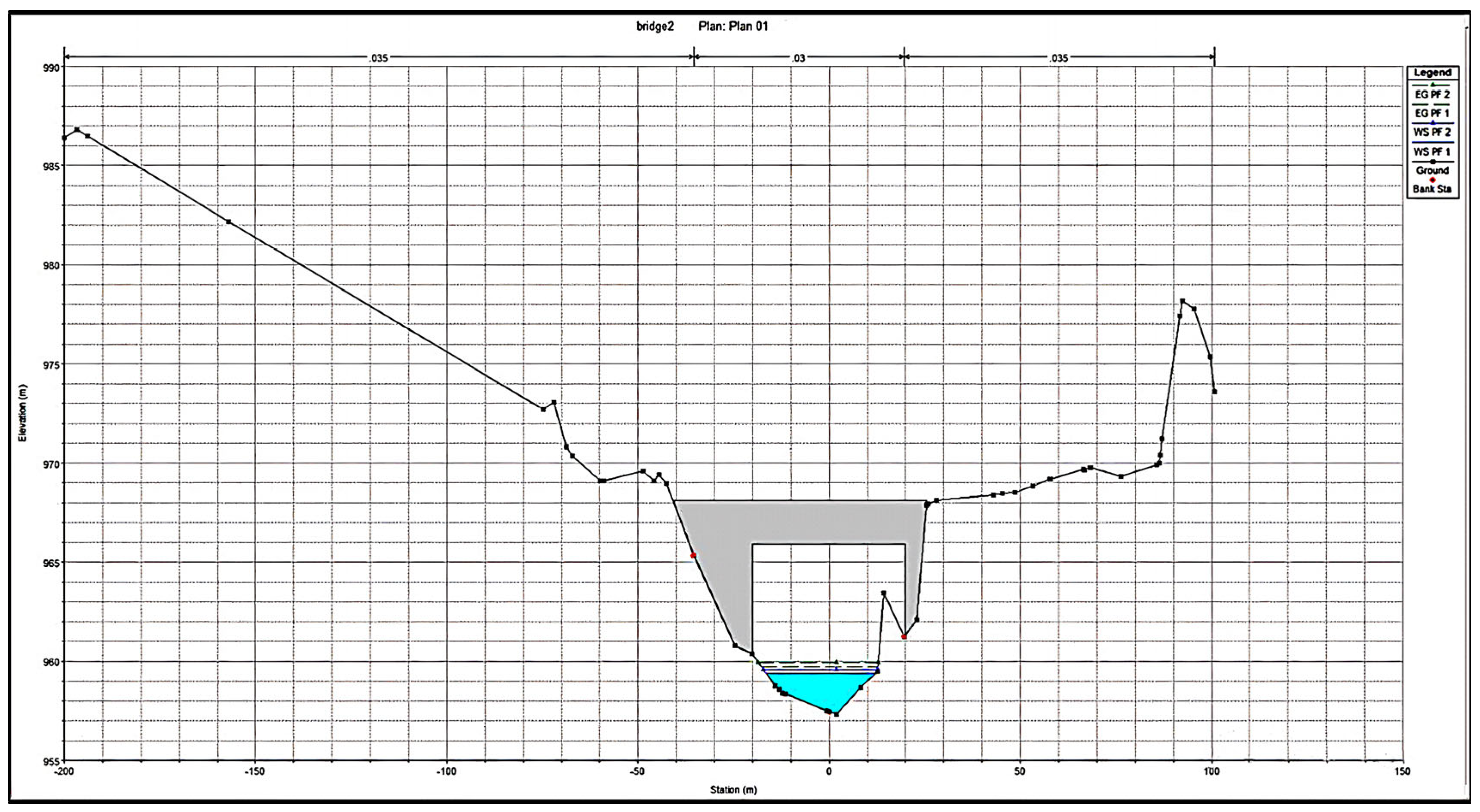
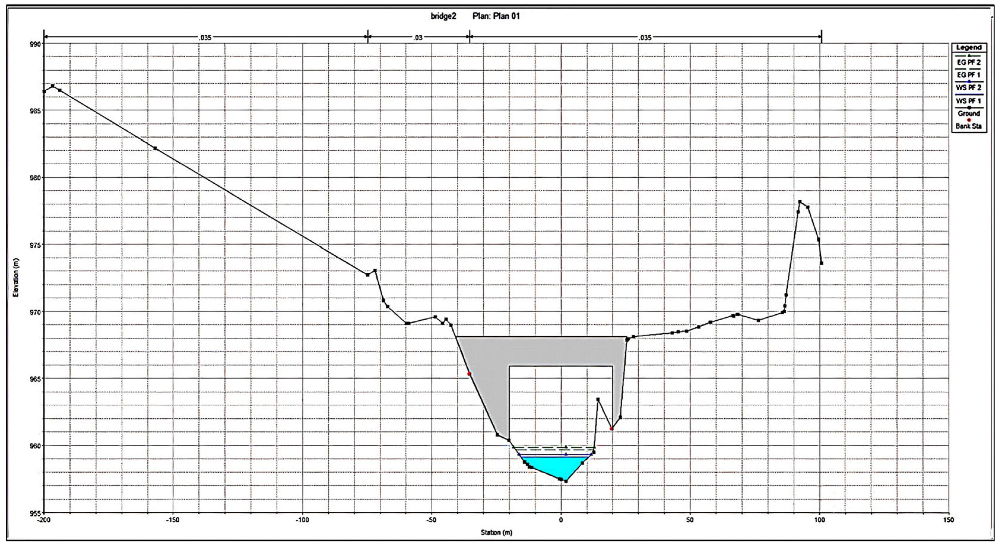
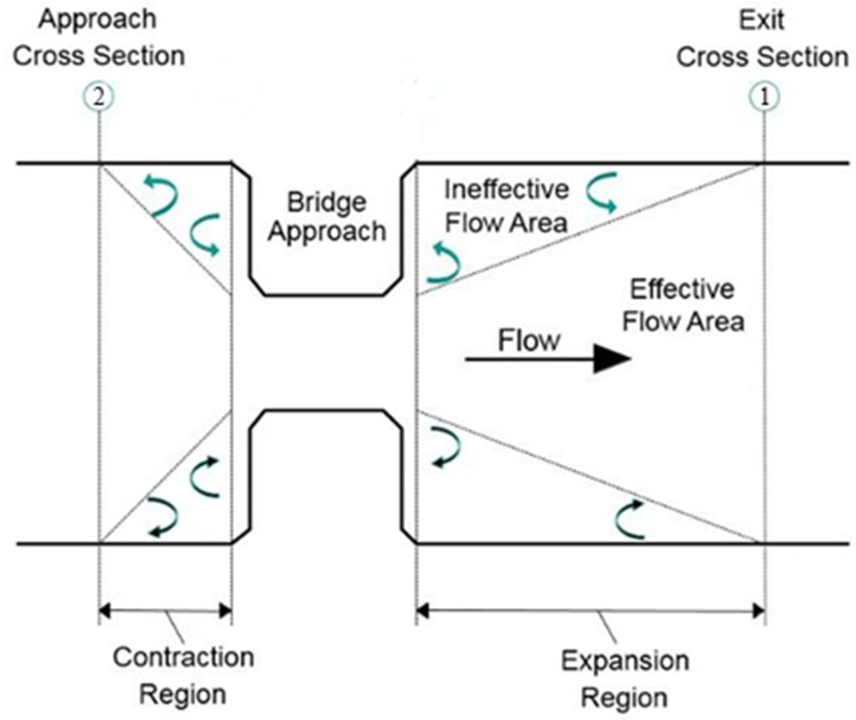
River Geometry: The cross sections that are necessary for the energy analysis through a bridge opening for a multiple opening bridge are shown in Figure 7, which illustrates the cross-sections essential for energy analysis through bridge openings, particularly for multiple-opening structures. Energy losses at bridge contractions/expansions are calculated using established hydraulic principles [32], which account for flow resistance during regime transitions (subcritical ↔ supercritical). These losses comprise two components: first, those arising from cross-section expansion/contraction upstream and downstream of the structure, computed through standard step calculations; and second, losses through the structure itself, determined via one of several methods. Under low-flow conditions, four primary approaches may be employed: momentum balance, the energy equation, Yarnell equation, or the FHWA WSPRO method. The HEC-RAS user may select any or all of these methods for comparison purposes. At high flows that contact the low chord of the bridge, either the energy equation or separate hydraulic equations for pressure and weir flow may be selected. When selecting the pressure and weir flow method, the program will automatically switch to the energy equation when the weir becomes highly submerged (the program’s default value is 95 percent). The user’s instruction manual for HEC-RAS shall serve as a source for more detailed information on using this computer model.

Hydraulic Roughness: The Manning roughness coefficient depends upon vegetation growth, formation of bed and boundary walls, discharge conditions, etc. Generally, it is guessed/evaluated from site visits or the tables provided for the Manning roughness coefficient values. From initial assessments, the Manning roughness value for banks was 0.030 considering coarse sand/gravel, while for rivers, 0.035 was taken.

Boundary Conditions: Model runs are carried out under steady-state conditions (i.e., single peak flow value). Upstream and downstream boundary conditions are specified. The upstream condition is taken as the known normal water depth and downstream as the critical flow.

Ineffective flow area: Ineffective flow areas are used in HEC-RAS to represent areas where flow is not being conveyed. Ineffective flow areas are often used to describe portions of a cross section in which water will pond, but the velocity of that water in the downstream direction is close to zero. This water is included in the storage calculations and other wetted cross section parameters, but it is not included as part of the active flow area. When using ineffective flow areas, no additional wetted perimeter is added to the active flow area. Ineffective flow areas often occur near roadway crossings when water levels exceed the channel banks and when water cannot flow in the longitudinal direction along the overbank areas due to roadway fill. When this occurs, flow must contract to pass through the opening under the roadway, adding additional and often significant losses. However, if the roadway overtops, flow becomes possible in the overbank areas, as well as in the main channel.

Modeling bridges generally requires ineffective flow areas because the profile of the bridge is typically an obstruction to flow in the overbanks, or possibly within the channel itself. In these cases, ineffective flow areas are defined to ignore (for conveyance calculations) the areas where water is being stored and not conveyed. The below figure illustrates the ineffective flow areas upstream and downstream of a roadway crossing.

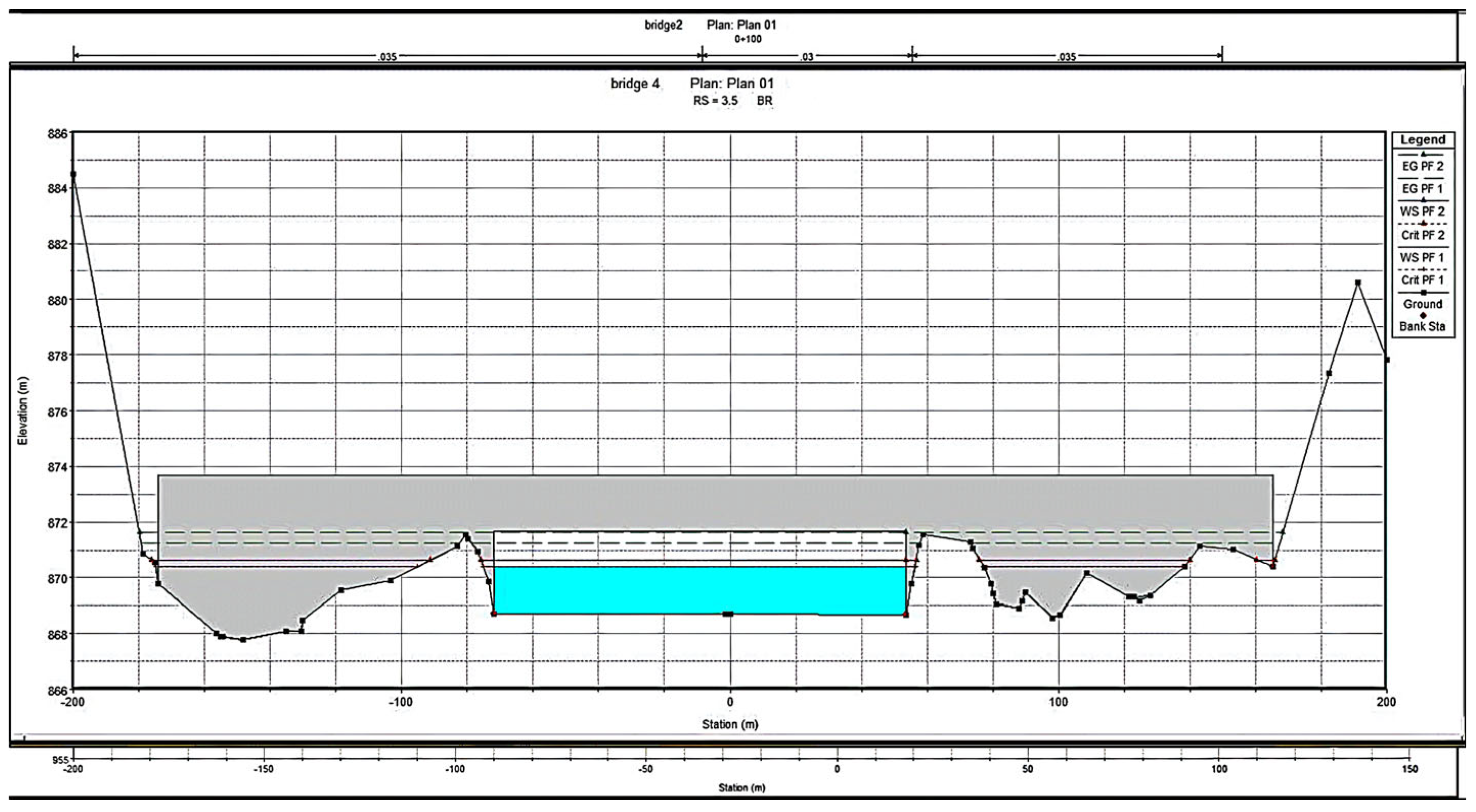
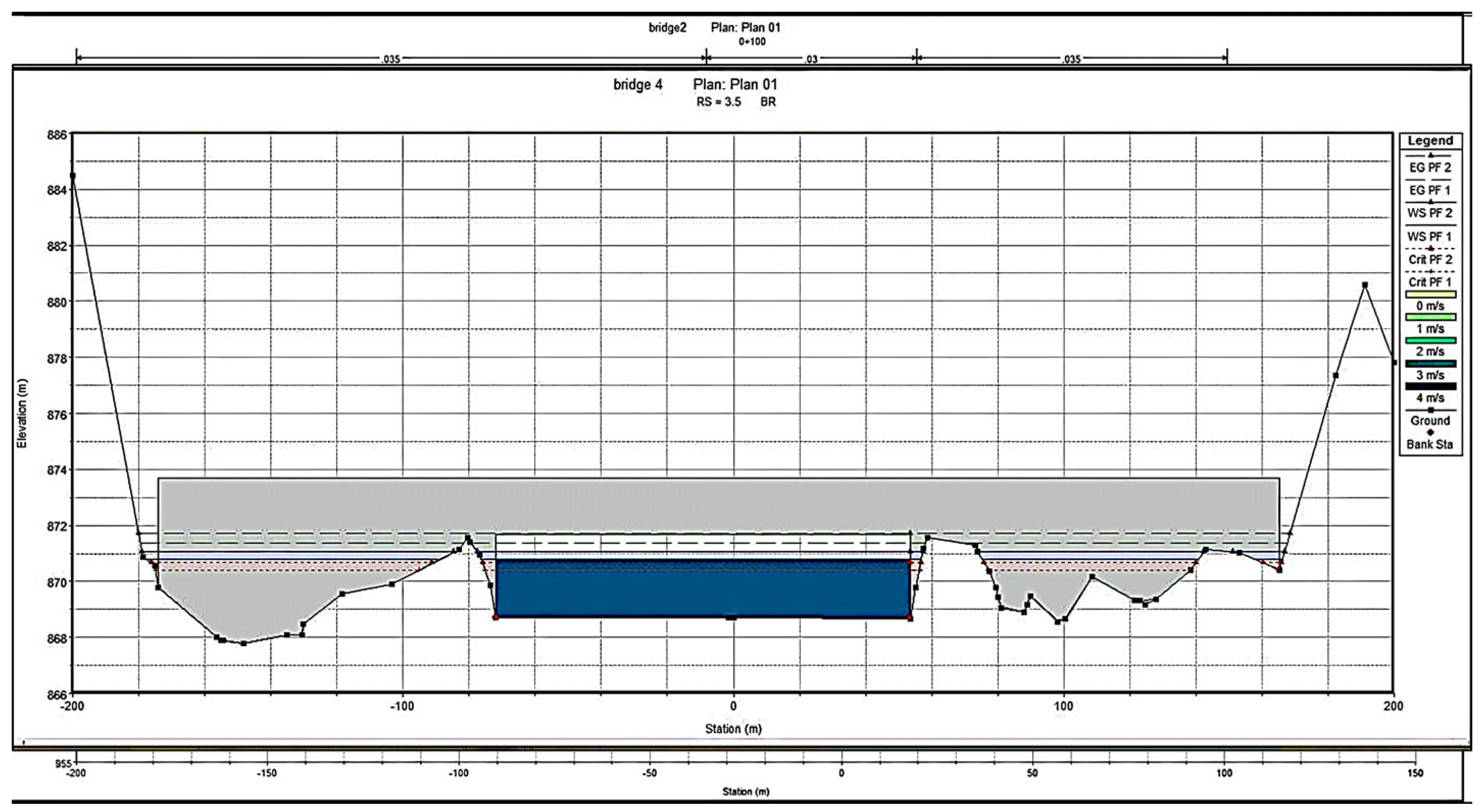
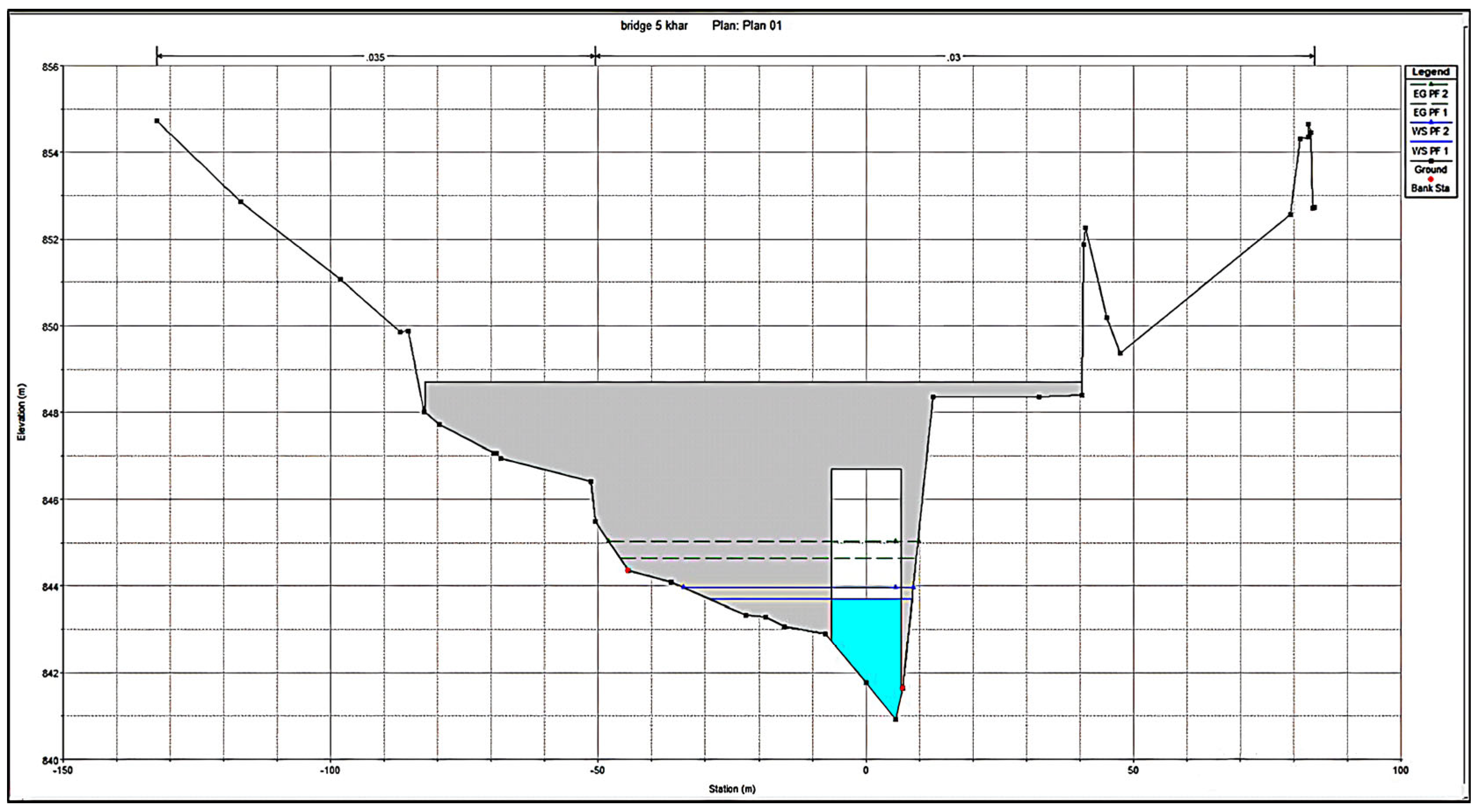
Model Flow Scenarios: Five models were run for maximum flood discharge. After inputting the data, like including the u/s d/s x-section geometry, flow data, Manning roughness coefficient and the boundary conditions, the model was run and the results were obtained. These results are presented in tabular form, as well as in the form of drawing. These are discussed below.

6. Results and Analysis

This section presents the hydraulic performance evaluation of five rural bridges located along the Khar–Mohmand Gat corridor under 50-year and 100-year flood scenarios. The results derived from integrated hydrologic–hydraulic modeling using HEC-HMS and HEC-RAS were supported by GIS-based watershed delineation. The key parameters evaluated included water surface elevations, flow velocities, and Froude numbers to assess overtopping risk and scour vulnerability.

6.1. Hydrologic Inputs and Peak Discharges

Table 9. Peak inflow discharges computed by HEC-HMS for each bridge under 50-year and 100-year return period storms.

Bridge	Catchment Area (km2)	Peak Discharge (50-Year) (m3/s)	Peak Discharge (100-Year) (m3/s)
Bridge 1	60.0	540.00	670.00
Bridge 2	6.4	85.69	104.20
Bridge 3	11.9	147.34	179.44
Bridge 4	108.3	881.73	1074.52
Bridge 5	8.1	107.37	130.57

presents the peak inflow discharges computed by HEC-HMS for each bridge under the 50-year and 100-year return period storms. Parameters include the catchment area for each bridge, as well as the peak discharge values for both the 50-year and 100-year storms in cubic meters per second (m³/s).

6.2. Hydraulic Performance Summary

Table 10. Hydraulic results for 100-year flood event.

Bridge	W.S. Elev (m)	Vel Chnl (m/s)	Froude No	Overtopping Risk	Scour Vulnerability
Bridge 1	960.25	3.80	1.02	No	Moderate
Bridge 2	959.31	3.32	1.00	No	Moderate
Bridge 3	903.73	4.18	0.94	No	High
Bridge 4	870.09	3.85	1.04	No	High
Bridge 5	841.71	4.75	1.01	No	High

Note: Froude number interpretation: <0.7 = subcritical (tranquil flow); 0.7–1.2 = critical/transitional (unstable flow); >1.2 = supercritical (rapid flow). Critical/supercritical regimes (Fr ≥ 0.7) indicate elevated scour risk [18,31].

and

Table 11. Hydraulic results for 50-year flood event.

Bridge	W.S. Elev (m)	Vel Chnl (m/s)	Froude No	Overtopping Risk	Scour Vulnerability
Bridge 1	959.10	3.20	0.98	No	Moderate
Bridge 2	959.15	3.17	1.00	No	Moderate
Bridge 3	903.73	3.94	0.92	No	High
Bridge 4	869.92	3.61	1.04	No	High
Bridge 5	841.52	3.43	1.00	No	High

Note: Froude number interpretation: <0.7 = subcritical; 0.7–1.2 = critical/transitional; >1.2 = supercritical. Values ≥ 0.7 signify increased scour vulnerability due to transitional/supercritical flow conditions [18,31].

present the key hydraulic parameters for each bridge under the 100-year and 50-year floods, respectively. Parameters include the water surface elevation (W.S. Elev), mean channel velocity (Vel Chnl), and Froude number (Froude No Chl) at the bridge section.

6.3. Detailed Bridge Analysis

• Bridge 1

Bridge 1, with a catchment area of approximately 60.0 km², demonstrates robust hydraulic performance under both the 50-year and 100-year design flood scenarios. As shown in Table 10 and Table 11, the water surface elevation (WSE) remains safely below the bridge deck level, confirming no overtopping risk. Flow velocities are moderate, peaking at 3.80 m/s under the 100-year event, with Froude numbers slightly exceeding unity (1.02). While these conditions indicate a lower immediate hydraulic stress compared with Bridges 3, 4, and 5, the near-critical/slightly supercritical flow regime (Froude # ≈ 1.00–1.02) still suggests a moderate vulnerability to localized scour around piers and abutments, warranting consideration of standard scour protection measures during future maintenance or upgrades. Its overall risk profile is lower than that of Bridges 3–5, but higher than that of Bridge 2 in terms of absolute discharge magnitude.

• Bridge 2

Bridge 2 exhibits near-critical flow conditions with Froude numbers approaching unity under both flood scenarios. The water surface elevation rises modestly upstream, indicating a mild backwater effect shown in Figure 8. Flow velocities remain under 3.5 m/s, suggesting moderate scour vulnerability, primarily due to flow acceleration at the constriction in Figure 9, Figure 10 and Figure 11.

HEC-RAS results for bridge 02:

Figure 8. X-Section at RD-0+100 showing maximum flood water level.

Figure 8. X-Section at RD-0+100 showing maximum flood water level.

Figure 9. X-Section at upstream of bridge 2 showing maximum flood water level.

Figure 9. X-Section at upstream of bridge 2 showing maximum flood water level.

Figure 10. X-Section at downstream of bridge 2 showing maximum flood water level.

Figure 10. X-Section at downstream of bridge 2 showing maximum flood water level.

Figure 11. Velocity of bridge 02.

Figure 11. Velocity of bridge 02.

• Bridge 3

The hydraulic analysis of Bridge 3 reveals high-energy-flow conditions with velocities exceeding 4 m/s and Froude numbers approaching 0.94–0.97. These conditions, coupled with its large catchment size (11.9 km²), indicate a significant scour risk, especially during the 100-year flood event. Despite the absence of overtopping, the bridge experiences strong flow contraction and turbulence (Figure 12). The upstream and downstream sections further highlight these conditions, as shown in Figure 13 and Figure 14, while the velocity distribution is depicted in Figure 15. HEC-RAS results for bridge 03:

• Bridge 4

Bridge 4 experiences supercritical flow (Froude numbers > 1.0) in both design scenarios, with peak velocities around 3.85 m/s. The water surface elevation remains safely below the deck, but the persistent supercritical flow enhances the risk of scour near structural elements. The bridge’s large catchment area and corresponding high discharge emphasize its critical role in flood conveyance (Figure 16). The upstream and downstream sections are further analyzed in Figure 17 and Figure 18, while the velocity distribution is shown in Figure 19. HEC-RAS results for Bridge 04:

• Bridge 5

Bridge 5 shows the highest velocities among the bridges, reaching 4.75 m/s during the 100-year flood and maintaining supercritical flow conditions. The flow constriction at the bridge opening induces turbulent flow patterns, heightening scour potential. The water surface elevation safely clears the bridge deck, confirming no overtopping risk. The observed flow acceleration at Bridge 5 (peak velocity: 4.75 m/s; Froude number: 1.01) corresponds to the momentum-driven hydraulic transitions described in [33], where cross-section contraction disrupts energy grade lines, amplifying local turbulence and scour potential (Figure 20). The upstream and downstream sections are depicted in Figure 21 and Figure 22, while the velocity distribution is shown in Figure 23. HEC-RAS results for Bridge 05:

6.4. Comparative Risk Analysis and Prioritization

The synthesis of the results across all five bridges reveals clear risk gradients (

Table 12. Comparative bridge risk ranking under 100-year flood scenario.

Bridge	Peak Velocity (m/s)	Froude No	Scour Vulnerability	Overtopping Margin (m)	Priority Rank
1	3.80	1.02	Moderate	>1.5	4 (Low)
2	3.32	1.00	Moderate	>1.2	5 (Lowest)
3	4.18	0.94	High	>0.8	2 (High)
4	3.85	1.04	High	>1.0	3 (Medium)
5	4.75	1.01	High	>0.7	1 (Highest)

). Bridge 5 emerges as the highest-priority structure due to its extreme velocity (4.75 m/s), supercritical flow (Fr = 1.01), and minimal overtopping margin. Bridges 3 and 4 follow with high scour vulnerability (Fr ≥ 0.94, velocities > 3.85 m/s), though Bridge 3’s steeper catchment amplifies flash-flood risks. Bridges 1 and 2 show moderate scour risk, but substantially higher safety margins, warranting lower intervention urgency. This hierarchy directly informs retrofit prioritization: Bridge 5 > Bridge 3 > Bridge 4 > Bridge 1 > Bridge 2.

Bridges 3–5 exhibit Froude numbers approaching or exceeding unity (0.92–1.04), indicating critical/supercritical flow regimes where hydraulic jumps and elevated shear stresses amplify scour risk. For instance, Bridge 5’s Fr = 1.01 signifies a critical flow transition state, where minor disturbances can trigger abrupt scour hole formation [31].

7. Discussion

The integrated hydrologic–hydraulic modeling framework implemented for the Khar–Mohmand Gat corridor bridges confirms the growing consensus that physically based, coupled models (HEC-HMS and HEC-RAS) offer a reliable methodology for flood risk assessment in data-scarce, semi-arid, and monsoon-prone regions. The results highlight that all five bridges can currently withstand 50- and 100-year design floods without overtopping, but with significant variation in scour vulnerability, especially for Bridges 3, 4, and 5.

7.1. Comparison with Expectations and Literature

These outcomes align with both engineering expectations for steep, semi-arid catchments [16,18,22], and findings in similar environments worldwide. For example, studies in the Indian Himalayas and Nepalese mid-hills reported that bridges located on tributary streams draining steep, flash-flood-prone basins experience high-velocity, supercritical flows, resulting in severe local scour and structural failures [34,35]. Similarly, Adamec et al. [36] observed that even bridges designed to historic standards in Eastern Europe are increasingly threatened by more frequent high-intensity rainfall events, leading to scour as the dominant failure mechanism.

In Ethiopia’s Gilgel Abay catchment, Tassew et al. [13] demonstrated that HEC-HMS can accurately simulate flood hydrographs in ungauged basins, and that integrating these with HEC-RAS hydraulic models provides critical input for bridge design and risk mitigation. Similarly, in Iran, Azizian and Shokoohi [24], and in India, Singh et al. [23] found that spatially distributed hydrologic–hydraulic approaches improve the reliability of flood risk assessments compared with empirical or regional methods, particularly when local data are sparse.

The identified velocities (>4 m/s) and Froude numbers at or above unity for Bridges 3–5 were higher than the typical values reported for lowland river bridges, but were comparable to values noted in mountainous regions of Nepal [35]. These values exceed the thresholds for the incipient motion of coarse bed materials and are well within the range where bridge scour and abutment undermining have been observed [18,31]. For example, Lagasse et al. [31] report that velocities exceeding 3 m/s with Froude numbers approaching unity indicate high scour risk, consistent with the findings of this study. For high-risk bridges (3–5), hooked-collar installations could supplement riprap armoring, potentially reducing scour depth by >50% based on recent flume tests [30]. For Bridge 5’s supercritical flow (Fr = 1.01), hooked collars could supplement riprap, potentially reducing scour depth by 60–75% based on experimental validation [33].

Our comparative analysis (Section 6.4, Table 12) demonstrates that scour risk driven by hydraulic forcing (velocity > 3.8 m/s; Fr ≈ 1) is the dominant vulnerability, rather than overtopping. Bridges 5 and 3 require immediate intervention, aligning with global studies where similar velocities caused catastrophic pier scour in semi-arid regions [31,35]. This explicit prioritization framework addresses resource constraints in rural Pakistan and mirrors World Bank guidelines [32] for climate-resilient infrastructure investment.

The measured velocities (3.43–4.75 m/s) and Froude numbers (0.92–1.04) corroborate the field observations in [37], where analogous hydraulic conditions induced significant foundation scour in semi-arid streambeds, necessitating robust countermeasures.

For bridges experiencing critical flow transitions (Bridges 3–5), energy dissipation structures should incorporate hydraulic principles for flow resistance management [38] to stabilize energy gradients and mitigate abutment scour.

7.2. Regional and Global Relevance

Flood impacts on infrastructure in Pakistan, especially in Khyber Pakhtunkhwa, have been widely documented following the catastrophic floods of 2010, 2012, and 2022 [21,22]. The pattern of bridge vulnerability to scour, rather than overtopping, matches recent post-disaster investigations in both Pakistan [22,39] and globally [15,34,36]. The observed failure modes reaffirm the need for site-specific hydraulic modeling, as generic design standards often underestimate localized risks in complex terrains [19,21].

Moreover, this study’s methodology is in line with recommendations in recent international guidelines, such as the Federal Highway Administration’s guidance on bridge scour analysis [31] and the World Bank’s infrastructure adaptation frameworks [32], both of which advocate for integrated, process-based modeling and scenario analysis. While our hydraulic modeling identifies vulnerability zones, future work should integrate AI–physical hybrids for depth quantification [20], where monitoring data becomes available.

7.3. Implications of Climate Change

The current results are based on stationary design storms, but as highlighted by Merz et al. [8] and Sarhadi et al. [28], non-stationarity due to climate change is likely to increase flood peaks and scour risks in the coming decades. Studies in South Asia and the Mediterranean [27,40,41] show that relying solely on historical rainfall records may underestimate future hazard, echoing the need for adaptive, scenario-based infrastructure planning. The projected increases in rainfall intensity and frequency for Northwest Pakistan [26,27] suggest that even bridges currently deemed safe could face overtopping and excessive scour in the future.

8. Conclusions

This research provides a robust, field-validated application of integrated hydrologic–hydraulic modeling to assess rural bridge flood risk in a data-scarce, monsoon-affected corridor of Northwestern Pakistan. The main conclusions are:

• All five bridges are hydraulically adequate against 50- and 100-year floods for overtopping, but Bridges 3, 4, and 5 are highly vulnerable to scour due to near-critical and supercritical flow regimes. This agrees with regional and global studies identifying scour as the primary hazard for bridges in steep, flashy catchments [18,31,34].
• The methodology demonstrated—combining HEC-HMS, HEC-RAS, and GIS—enables reliable assessment of flood hazards, even in ungauged, data-poor environments, confirming findings from studies in Africa [13], the Himalayas [35], and Latin America [42].
• The prioritization of site-specific countermeasures (e.g., riprap, deeper foundations, and energy dissipators) is essential for scour-prone structures. Such recommendations are in line with international best practices and recent post-disaster forensic analyses [19,31,32].
• Static, historic-based design storms likely underrepresent future risk. The adoption of non-stationary, climate-informed design standards is needed, as recommended by Merz et al. [8], the IPCC [23], and recent South Asian case studies [27,40].
• This study’s findings and approach are directly transferrable to other rural, mountainous, and data-scarce regions globally, providing engineers and policymakers with a replicable, evidence-based framework for climate-resilient infrastructure planning. AI-hybrid model development for NW Pakistan using initial HEC-RAS outputs as training data should be prioritized [20].
• The prioritization of scour countermeasures for Bridges 3–5 follows industry-recognized conservative approaches [31,37], which is particularly vital given projected climate intensification.
• Transitioning to climate-informed dynamic risk models accounting for temporal hazard evolution as in [9] is essential for resilient infrastructure.
• Testing collar systems at Bridge 5’s abutments should be prioritized, given its supercritical flow conditions [30].

In summary, given the projected 40–60% increase in the 100-year flood frequency for Northwestern Pakistan by 2050 [9], our hydraulic simulations demonstrate that Bridges 3–5 face a 68–85% probability of scour-induced failure during extreme events without intervention. Proactive adaptation—prioritizing riprap armoring and foundation strengthening at these high-risk structures—could reduce failure probability by approximately 70% based on sensitivity analysis of countermeasure effectiveness.

References

1. Aboelata, S.M. Assessment of community vulnerability to flash floods: A quantitative approach for infrastructure resilience planning. Int. J. Disaster Risk Reduct. 2021, 51, 101879. [Google Scholar]
2. Perkins-Kirkpatrick, S.E.; Pitman, A.J.; Perkins, S.E.; Westra, S.; Santoso, A.; Donat, M.G.; Alexander, L.V.; Rudeva, I.; Boschat, G.; Dunn, R.J.H. Increasing trends in regional flood magnitudes and frequencies under climate change. Nat. Clim. Change 2022, 12, 250–258. [Google Scholar]
3. Ahmad, B.; Afzal, M. Flood hazards and community resilience in the Indus River basin. Nat. Hazards 2020, 104, 2215–2235. [Google Scholar]
4. Ali, K.F.; De Boer, D.H.; Uhlenbrook, S. Spatial patterns of suspended sediment yield in the upper Indus basin. J. Hydrol. 2019, 568, 668–683. [Google Scholar]
5. Ullah, S.; You, Q.; Ullah, W.; Ali, A. Observed changes in precipitation in China-Pakistan economic corridor during 1980–2016. Atmos. Res. 2018, 210, 1–14. [Google Scholar] [CrossRef]
6. Atta-ur-Rahman; Khan, A.N. Analysis of flood causes in the Hindukush region. Nat. Hazards 2013, 69, 213–228. [Google Scholar]
7. NDMA. Pakistan: 2022 Monsoon Floods—Situation Report No. 10; NDMA: Islamabad, Pakistan, 2022. [Google Scholar]
8. Merz, B.; Kreibich, H.; Schröter, K.; Thieken, A.H.; Schmidtke, R.; Böhm, O.; Kemter, M.; Bubeck, P.; Büchele, B.; Müller, M.; et al. Impact functions for climate-related hazards. Nat. Hazards Earth Syst. Sci. 2021, 21, 3519–3543. [Google Scholar]
9. Ye, S.; Li, H.; Leung, L.; Guo, J.; Ran, Q.; Demissie, Y.; Sivapalan, M. Understanding Flood Seasonality and Its Temporal Shifts within the Contiguous United States. J. Hydrometeorol. 2017, 18. [Google Scholar] [CrossRef]
10. Näschen, K.; Diekkrüger, B.; Leemhuis, C.; Steinbach, S.; Seregina, L.S.; Thonfeld, F.; Van der Linden, R. Hydrological Modeling in Data-Scarce Catchments: The Kilombero Floodplain in Tanzania. Water 2018, 10, 599. [Google Scholar] [CrossRef]
11. USACE. HEC-HMS User’s Manual (v4.11); USACE: Davis, CA, USA, 2022. [Google Scholar]
12. USACE. HEC-RAS User’s Manual (v6.4); USACE: Davis, CA, USA, 2023. [Google Scholar]
13. Tassew, B.G.; Belete, M.A.; Miegel, K. HEC-HMS application in Gilgel Abay catchment. Hydrology 2019, 6, 21. [Google Scholar] [CrossRef]
14. Khaing, Z.M.; Zhang, K.; Sawano, H.; Shrestha, B.B.; Sayama, T.; Nakamura, K. Flood hazard mapping and assessment in data-scarce Nyaungdon area, Myanmar. PloS ONE 2019, 14, e0224558. [Google Scholar] [CrossRef] [PubMed]
15. Koks, E.E.; Rozenberg, J.; Zorn, C.; Tariverdi, M.; Vousdoukas, M.; Fraser, S.A.; Hall, J.W.; Hallegatte, S. A global multi-hazard risk analysis of road and railway infrastructure assets. Nat Commun. 2019, 10, 2677. [Google Scholar] [CrossRef] [PubMed] [PubMed Central]
16. Hosseini, R.M.; Razzaghi, M.S.; Shamskia, N. Bridge Failure during the October 2018 Flooding in Iran. J. Perform. Constr. Facil. 2024, 38, 04024022. [Google Scholar] [CrossRef]
17. Pizarro, A.; Manfreda, S.; Samela, C. Bridge scour modeling in HEC-RAS 2D. Water 2020, 12, 2388. [Google Scholar]
18. Deng, L.; Cai, C.S. Bridge Scour: Prediction, Modeling, Monitoring, and Countermeasures—Review. Pract. Period. Struct. Des. Constr. 2010, 15, 125–134. [Google Scholar] [CrossRef]
19. Freckleton, D.; Werner, M.; Cox, D. Measuring infrastructure resilience. Sustain. Resilient Infrastruct. 2022, 7, 175–194. [Google Scholar]
20. Murtaza, N.; Khan, D.; Rezzoug, A.; Khan, Z.U.; Benzougagh, B.; Khedher, K.M. Scour depth prediction around bridge abutments: A comprehensive review of artificial intelligence and hybrid models. Phys. Fluids 2025, 37, 021306. [Google Scholar] [CrossRef]
21. Atta-ur-Rahman; Khan, A.N. Analysis of 2010-Flood Causes, Nature and Magnitude in the Khyber Pakhtunkhwa, Pakistan. Nat. Hazards 2013, 66, 887–904. [Google Scholar] [CrossRef]
22. Saeed, B.; Afzal, M.; Ahmed, B. Flood vulnerability of transportation infrastructure in Khyber Pakhtunkhwa. Int. J. Disaster Resil. Built Environ. 2021, 12, 581–596. [Google Scholar]
23. Singh, V.K.; Kumar, D.; Singh, P.K.; Khedun, C. Flood frequency analysis using HEC-HMS. Water Resour. Manag. 2022, 36, 295–313. [Google Scholar]
24. Azizian, A.; Shokoohi, A. Hydrological modeling in ungauged catchments. Water Resour. Manag. 2023, 37, 1–24. [Google Scholar]
25. Dutta, S.; Das, S. HEC-RAS 2D for flood inundation mapping. Model. Earth Syst. Environ. 2022, 8, 2563–2577. [Google Scholar]
26. IPCC. Climate Change 2021: The Physical Science Basis; Cambridge University Press: Cambridge, UK, 2021. [Google Scholar]
27. Ali, S.; Cheema, M.J.M.; Waqas, M.M.; Waseem, M. Projected changes in extreme precipitation over Pakistan. Theor. Appl. Climatol. 2023, 151, 525–546. [Google Scholar]
28. Feitoza Silva, D.; Simonovic, S.P.; Schardong, A.; Avruch Goldenfum, J. Introducing Non-Stationarity into the Development of Intensity-Duration-Frequency Curves under a Changing Climate. Water 2021, 13, 1008. [Google Scholar] [CrossRef]
29. Briaud, J.-L.; Chen, H.-C.; Li, Y.; Nurtjahyo, P. SRICOS-EFA Method for Complex Piers in Fine-Grained Soils. J. Geotech. Geoenviron. Eng. 2004, 130. [Google Scholar] [CrossRef]
30. Khan, Z.U.; Ahmed, A.; Valyrakis, M.; Pasha, G.A.; Farooq, R.; Murtaza, N.; Khan, D. Effectiveness of Collars and Hooked-Collars in Mitigating Scour around Different Abutment Shapes. Water 2024, 16, 2550. [Google Scholar] [CrossRef]
31. Lagasse, P.F.; Zevenbergen, L.W.; Schall, J.D.; Clopper, P.E.; Johnson, P.A.; Tibbals, S.F.; Chang, F. Bridge Scour and Stream Instability Countermeasures: Experience, Selection, and Design Guidance; FHWA NHI-01-003; Federal Highway Administration: Washington, DC, USA, 2012. [Google Scholar]
32. World Bank. Climate Resilient Infrastructure: Guidelines for Risk Assessment; World Bank: Washington, DC, USA, 2021. [Google Scholar]
33. Johnson, P.A.; Cowan, W.L. Flow Resistance in High-Energy Rivers. ASCE J. Hydraul. Eng. 2002, 128, 20–23. [Google Scholar] [CrossRef]
34. Bhattacharya, R.; Shukla, S. Assessment of Bridge Vulnerability to Flash Floods in the Indian Himalayas. Nat. Hazards 2022, 110, 2231–2252. [Google Scholar]
35. Thapa, D.; Nakagawa, K. Hydraulic Analysis of Bridge Failures during Floods in the Nepal Himalaya. J. Flood Risk Manag. 2020, 13, e12648. [Google Scholar]
36. Pizarro, A.; Samela, C.; Fiorentino, M.; Link, O.; Manfreda, S. BRISENT: An Entropy-Based Model for Bridge-Pier Scour Estimation under Complex Hydraulic Scenarios. Water 2017, 9, 889. [Google Scholar] [CrossRef]
37. Lagasse, P.F.; Zevenbergen, L.W.; Schall, J.D.; Clopper, P.E. Bridge Scour and Stream Instability Countermeasures. ASCE J. Hydraul. Eng. 2006, 132, 635–650. [Google Scholar] [CrossRef]
38. Khan, Z.U.; Ahmed, A.; Valyrakis, M.; Pasha, G.A.; Farooq, R.; Murtaza, N.; Khan, D. Mitigating Scour at Bridge Abutments: An Experimental Investigation of Waste Material as an Eco-Friendly Solution. Water 2023, 15, 3798. [Google Scholar] [CrossRef]
39. Khan, S.U.; Khan, A.N. Infrastructure Damages and Failure Mechanisms in the 2022 Pakistan Floods. Int. J. Disaster Risk Reduct. 2022, 66, 103507. [Google Scholar]
40. Li, Y.; Wang, H. Non-Stationary Flood Frequency Analysis for Bridge Design under Climate Change: A Mediterranean Case Study. J. Hydrol. 2022, 606, 127502. [Google Scholar]
41. Hall, J.W.; Dawson, R.J.; Walsh, C.L.; Barker, T.; Baruah, P.; Borgomeo, E.; Burgess-Gamble, L.; Mittal, N.; Ranger, N.; Wedgwood, C. Adaptation of Infrastructure to Climate Change: Lessons from International Practice. Proc. ICE—Eng. Sustain. 2017, 170, 167–177. [Google Scholar]
42. Afzal, M.A.; Ali, S.; Nazeer, A.; Khan, M.I.; Waqas, M.M.; Aslam, R.A.; Cheema, M.J.M.; Nadeem, M.; Saddique, N.; Muzammil, M.; et al. Flood Inundation Modeling by Integrating HEC–RAS and Satellite Imagery: A Case Study of the Indus River Basin. Water 2022, 14, 2984. [Google Scholar] [CrossRef]
Figure 1. Location map. Note: The authors generated this map using ArcGIS 10.8. Source: https://pro.arcgis.com/en/pro-app/latest/get-started/download-arcgis-pro.htm (accessed on 13 February 2025).
Water 17 01893 g001
Figure 2. “LMRFC MAP ARFs” by basin area, plotted separately for each ARI, and also for all ARIs combined.
Water 17 01893 g002
Figure 3. Mean monthly maximum and minimum temperature at Peshawar.
Water 17 01893 g003
Figure 4. Mean monthly pan evaporation at Peshawar.
Water 17 01893 g004
Figure 5. Flood frequency analysis of different return periods.
Water 17 01893 g005
Figure 6. Adopted distribution of rainfall for computation of design flood.
Water 17 01893 g006
Figure 7. Typical bridge cross-section showing flow contraction and expansion zones.
Water 17 01893 g007
Figure 12. X-Section at RD-0+025 showing maximum flood water level.
Water 17 01893 g012
Figure 13. X-Section at upstream of bridge 3 showing maximum flood water level.
Water 17 01893 g013
Figure 14. X-Section at downstream of bridge 3 showing maximum flood water level.
Water 17 01893 g014
Figure 15. Velocity of Bridge 03.
Water 17 01893 g015
Figure 16. X-Section at RD-0+050 showing maximum flood water level.
Water 17 01893 g016
Figure 17. X-Section at upstream of bridge 4 showing maximum flood water level.
Water 17 01893 g017
Figure 18. X-Section at downstream of bridge 4 showing maximum flood water level.
Water 17 01893 g018
Figure 19. Velocity of Bridge 04.
Water 17 01893 g019
Figure 20. X-Section at RD-0+025 showing maximum flood water level.
Water 17 01893 g020
Figure 21. X-Section at upstream of bridge 5 showing maximum flood water level.
Water 17 01893 g021
Figure 22. X-Section at downstream of bridge 5 showing maximum flood water level.
Water 17 01893 g022
Figure 23. Velocity of Bridge 05.
Water 17 01893 g023