Abstract
Wave propagation is impacted by the presence of ice floes. The influence of waves, on the other hand, causes ice floes to overlap and accumulate. In this paper, the interaction of ice floes and regular waves was simulated using the Finite Element Method. Firstly, natural ice floe fields were generated using the Python 3.10 programing language, with floe size distribution and randomness taken into consideration. Then, using the velocity inlet boundary wave generation method, regular simple harmonic waves were produced. The process where ice floes couple with waves was simulated with the Coupled Eulerian–Lagrangian (CEL) approach. Variations in wave height after passing through the ice floe field were investigated, and further research was conducted on the movement and fragmentation characteristics of ice floes. Simulations employing the Coupled Eulerian–Lagrangian (CEL) approach reveal that (1) ice floe motion exhibits periodic characteristics synchronized with incident wave periods; (2) wave height attenuation increases by 62–80% with rising ice concentration (70–90%); and (3) fragmentation predominantly occurs at wave trough phases due to flexural stress concentration. These findings quantitatively characterize wave–ice energy transfer mechanisms critical for polar navigation safety assessments.
1. Introduction
Global warming has accelerated the melting of sea ice in the Arctic, and sea ice cover has been decreasing year by year, with changes in sea ice extent observed since satellite observations began in 1979, with summer and autumn being the most significant, showing a reduction of about 50 percent. The feasibility of Arctic navigation by ships has increased significantly. The marginal ice zone is located between an ice sheet and open water, which is the area where ice floes are concentrated, and it is also the key area for polar ship navigation. According to an analysis by Li [1], in recent decades, the effective wave height and wave period in most areas of the Arctic Ocean in summer have increased, which means that the number of waves carrying more energy have increased. The interaction mechanism between wave and ice floes is the technical basis of ship–wave–ice floe coupling analysis and is an important part of evaluating the navigation safety of ships in the marginal ice zone. The interaction between waves and ice floes is an extremely complex fluid–structure interaction process, and research work on this involves the macroscopic physical morphology and mechanical properties of sea ice, as well as complex wave theory. Therefore, the coupling relationship between waves and ice floes is worthy of in-depth study.
In the early days, scholars mainly applied theoretical models of the interaction between waves and ice floes, such as the mass loading model proposed by Peters [2], the elastic sheet bending model proposed by Wadhams [3], and, subsequently, a series of models accounting for the viscosity of seawater. Luo [4] believes that theoretical models have their own advantages and are suitable for different scenarios; for example, the mass load model is mainly suitable for discontinuous lotus-leaf-like ice regions, the elastic sheet model is suitable for continuous ice sheets, the viscous layer model is mainly suitable for grease ice regions, and the viscoelastic model can be applied to the entire marginal ice zone with appropriate coefficients. Because the correlation coefficient of the viscoelastic model is difficult to determine by experimental measurements and other means, it is difficult to apply it directly.
In terms of experimental approaches, due to the complexity of the interaction between waves and ice floes, field observations and model experiments provide valuable insights. Specifically, field observations are often based on buoys, submersibles, and navigation but, due to the constraints of a harsh environment and poor accessibility, field observations are relatively few, and the time and space coverage is low. Typically, only the basic data of waves are obtained from field observations, and measurements of wave–ice floe interactions are rarely carried out. For example, Dean [4] used a ship-borne wave recorder to record the attenuation of waves in the ice margin region, while Rogers [5] observed the attenuation of waves in the floating ice region in the Beaufort Sea. Furthermore, indoor model tests are demanding and require both sea ice simulation and wave-making capabilities, and the Hamburg Ice Pool is one of the few ice pools with wave-making capabilities. Notably, with the support of the joint project LS-WICE, a series of wave–ice interaction model tests were carried out in HSVA [6,7], which involved the analysis of wave propagation and attenuation characteristics in sea ice regions, the motion characteristics of ice floes in waves, the breakage characteristics of level ice under wave action, and the structural ice load under the combined action of waves and ice floes. Due to the limitation of experimental conditions, Wang [8] used paraffin non-frozen model ice to simulate the size distribution of ice floes in real-world conditions, measured the motion response of ice floes in regular waves of different wavelengths, summarized their longitudinal and vertical motion responses, and compared them with the motion response laws of isolated ice floes in waves, and the results showed that the longitudinal motion of the ice floes in the waves showed two motion states: irregular motion in the short-wave interval and regular motion in the long-wave range.
Regarding numerical simulations, Meylan [9] studied the coupling effect of different shapes of sea ice under wave action and found that waves are most obviously affected by the bending stiffness of ice floes but have no obvious relationship with the geometry of ice floes. Wang [10] studied the interaction between waves and arbitrarily shaped elastic ice floes based on the coupled boundary element method, and the calculation results were consistent with Meylan’s conclusion. Wu [11] carried out numerical simulation studies of waves and single ice floes based on STAR-CCM+ and comprehensively analyzed the effects of thickness, size, and shape of ice floes on their motion characteristics in waves. Ni [12] used the VOF model to study the interaction characteristics of two-dimensional Stokes waves with single and multiple ice floes and analyzed the motion and force characteristics of ice floes under wave action, as well as the propagation characteristics of waves. Wang [13] studied the interaction between regular waves and ice floes based on the S-ALE method in LS-DYNA, focusing on the longitudinal drift motion of ice floes under wave action, analyzing the influence of the ratio of wavelength to the size of ice floes on the longitudinal drift motion characteristics of ice floes, and validating the numerical model based on model experiments. Lu [14] combined FLUENT with EDEM, simulating ice floes as discrete elements and waves using the VOF method. Wu [15] simulated the level ice failure under wave action based on the DEM-SPH coupling model, examining the effects of wave height, wave period, and ice thickness on ice failure mode. Zhang [16] developed a novel two-way SPH method incorporating a density-ratio-sensitive fluid–ice interaction model, an ice particle separation algorithm for fracture, and unequal time-step treatment. This method efficiently simulated wave-induced breakup of ice floes, was validated against regular waves experiments, and applied to solitary and focused waves. He [17] established a one-way CFD-DEM coupling model using FVM for waves and bonded DEM particles for ice. This model simulated ice sheet breakup under regular waves, was validated against HSVA experiments, and revealed nonlinear floe size distributions dependent on wave height and ice thickness. Zhang [18] developed an SPH model with an improved fluid–ice interface treatment scheme, using ice particles as dummy particles to simulate wave-induced kinematic responses and flexural deformations of ice floes, validated against experimental data for surge/heave motions and bending patterns. Ni [19] synthesizes research on ice deformation and fracture induced by flexural-gravity waves (FGWs) from both above-ice and underwater moving loads. This synthesis covered diverse ice conditions (intact sheets, cracks, leads, and channels) and explored factors like load velocity, ice properties, and boundary effects.
In summary, methodologies for studying wave–ice floe interactions include theoretical models, experimental observations, and numerical simulations. Among these, numerical simulation holds potential, enabling effective characterization of wave propagation and ice floe motion dynamics under wave action. Building on these advances, in this paper, the interaction between ice floes and waves is simulated based on the coupled Eulerian–Lagrangian method, with a focus on the motion and fragmentation characteristics of ice floes in waves, as well as the propagation and attenuation characteristics of waves within ice fields.
2. Basic Theory
2.1. CEL and Hydrodynamic Models
This work utilizes the explicit dynamics module of a finite element software platform, an industry-standard framework for simulating dynamic phenomena involving nonlinear processes such as high-speed collisions. Since the dynamical equations are in differential format, there is no need to perform equilibrium iterations. Computational convergence is inherently ensured when the sufficiently small time steps are employed. The equation of state that can describe fluid dynamics is introduced into ABAQUS/Explicit and, combined with the CEL method, enables robust simulation of fluid–structure interaction (FSI). In recent years, the CEL method has been extensively applied to FSI problems with significant success. For instance, Majlesi [20] employed the CEL method to simulate the interaction between waves and bridge piers and the simulation results were in good agreement with the experiments, and Kim [21] used the CEL method to simulate the tank fall study to analyze the impact of the fluid on the oil tank during the tank fall.
The CEL method employs distinct kinematic descriptions, the Eulerian formulation for fluids and the Lagrangian formulation for solids. In this work, waves are modeled within a Eulerian domain, while ice floes are represented using a Lagrangian mesh. Interaction between these domains is governed by the principles of the immersed boundary method. A dedicated fluid–structure interaction (FSI) contact algorithm defines the influence of the Lagrangian body (ice floe) motion on the Eulerian domain (fluid), coupling Eulerian elements with Lagrangian elements for simultaneous solution. Figure 1 illutrates the Lagrangian body and Eulerian body within the velocity field. Crucially, the Lagrangian mesh deforms and displaces congruently with the material it represents (the ice floe). Conversely, the Eulerian mesh remains spatially fixed; material deformation and flow within this domain are tracked via the evolving volume fraction of material within each cell, calculated using the VOF method.
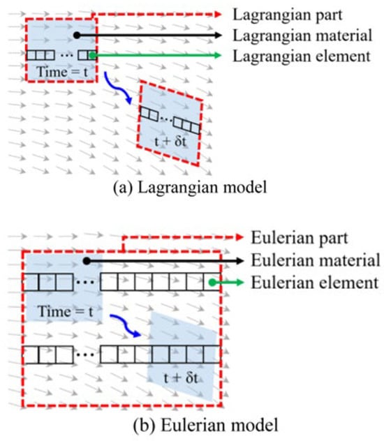
Figure 1.
Schematic representation of Lagrangian and Eulerian frameworks [21].
The Eulerian framework, characterized by its non-deforming mesh, circumvents mesh distortion issues inherent in Lagrangian methods. This makes it particularly suitable for simulating large material deformations. Consequently, wave simulation in this study is implemented within the Eulerian domain. The governing equations for the fluid are given by the conservation laws:
where ρ is the density, f is the density of the external force, v is the velocity vector, and e is the specific internal energy. The water body is described by the Mie–Grüneisen equation of state in the form of a linear Us-Up Hugoniot.
where is pressure, is specific energy, is linear shock wave velocity, is particle velocity, is speed of sound, and are reference material constants, and is the viscosity coefficient.
2.2. Wave Generation Method
In this study, the fluid domain is modeled using the Eulerian approach. Periodic waves are generated by prescribing a time-dependent velocity boundary condition along the Eulerian domain boundary. Consistent with wave theory, these periodic waves are fully characterized by three independent parameters, wave height H, period T, and water depth h, as shown in Figure 2. Referring to the research conclusions of Montoya [22], it is possible to generate ideal Stokes second-order waves through Equations (6)–(11). When the wave height is too large relative to the water depth, the wave is prone to breakage, so the relevant parameters of the wave need to meet Equations (12) and (13).
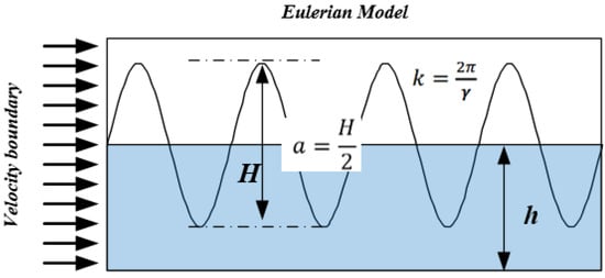
Figure 2.
Periodic wave schematic.
In the formula, references the displacement boundary that should be applied since the Euler body only supports the definition of velocity boundary, v can be used to generate an ideal wave, is the wave number, is circular frequency, is theoretical wave free surface, is wave length, and the other parameters are process physical quantities.
2.3. Generation of the Ice Floe and Material Model of Sea Ice
The temporal and spatial distribution of Arctic ice floes is quite random, and the distribution rules of ice floes in different sea areas vary greatly and have pronounced seasonal/interannual characteristics. The distribution data of ice floes are primarily derived from satellite imagery, aerial surveys, and ship navigation photography equipment. Limited to factors such as resolution and measurement range, there is no unified function expression of the distribution law of ice floe at present. Consequently, this study generates ice floe fields assuming a normal size distribution. ABAQUS has a flexible secondary development interface, which can be implemented through the scripting language Python. At present, the generation methods of ice floe mainly include the polygon overlap method, Vino cutting method, and image recognition method. Among them, the polygon overlap method can generate arbitrary shaped ice floe blocks, and it is convenient to adjust the size distribution law and roundness of ice floe blocks, but the time complexity is high when the program is designed, and the overlap probability of polygons is too high when the density is high, so the generation efficiency of the high-density ice floe field is low. The image recognition method requires the input of a high-quality target image, and accurate contour segmentation becomes challenging with low image quality or contacting floes. Therefore, this paper generates an ice floe based on the Wino polygon function in Python, firstly by adjusting the arrangement of the Vino seeds, changing the size distribution of the ice floe, then scaling the ice floe in equal proportions to make the ice floe density reach the specified value, and finally extracting the corner coordinates of the ice floe to construct the ice floe through the ABAQUS built-in function. As shown in Figure 3, 90%, 70%, and 50% concentration ice floes were generated, and the area of each ice floe was statistically fitted, and it was found that its size distribution was normally distributed, which met the expectations of the program design.
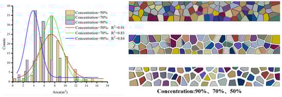
Figure 3.
Generated ice fields at 90%, 70%, and 50% concentrations.
Ice floes may break up under the action of waves, which is closely related to the size of the ice floes, etc. With the development of computer technology and algorithms, it has become common to use FEM to analyze material fracture failure, and the most common method for simulating failure is the element deletion model. Before the damage starts, the mechanical behavior of the material obeys the preset constitutive model and, when the damage starts, the stiffness of the material degrades until the bearing capacity is completely lost and the element is deleted, which is macroscopically manifested as a crack. In summary, when using the element deletion model, it is necessary to set the constitutive model, the damage initiation criterion, and the element failure criterion. In this paper, the pre-damage initiation model follows the Drucker Prager plastic model, which exhibits strain-hardening behavior after yielding, and the material begins to damage and stiffness degrades when the equivalent plastic strain reaches a certain value. The Drucker Prager plastic model introduces the effect of hydrostatic pressure into the Mises yield criterion.
When this criterion is applied to yield, there are usually three yield surface forms, namely linear form, hyperbolic form, etc.; as shown in Figure 4a, a simple linear form is selected, which provides a yield surface in the partial plane that cannot be circular to match the different yield values of triaxial tension and compression, the associated inelastic flow in the partial plane, and the separate expansion and friction angles. is the cohesive term of Drucker Prager’s model, p is the hydrostatic pressure, β is the friction angle, and t is the Mises equivalent stress.
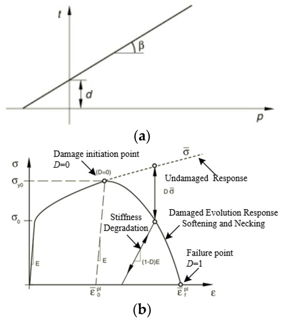
Figure 4.
The constitution of sea ice materials. (a) Drucker Prager plastic; (b) ductile damage.
3. Numerical Simulation and Analysis
Following the methodology established in Section 2, this section first carries out the verification of the wave generation method and then simulates the interaction between the wave and the ice floe based on the CEL method and then analyzes the propagation and attenuation characteristics of the wave in the ice floe area, as well as the movement and failure characteristics of the ice floe under waves action, as shown in Figure 5.
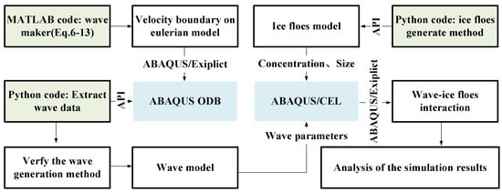
Figure 5.
Framework of the numerical simulation.
3.1. Wave Generation and Verification
According to the wave generation theory in Section 2.2, the simulation prescribed a wave height H = 1, period T = 5 s, and initial water depth h = 8 m. The time-dependent velocity boundary condition, generated using MATLAB R2016b, was applied to specific boundaries of the Eulerian domain as illustrated in Figure 6. The velocity boundary condition and Euler boundary condition are set on the YZ plane, wherein the non-reflection boundary condition can reduce the reflection of the fluid and ensure the wave surface height. The Euler boundary condition is set on the upper surface of XY to simulate the atmosphere, and the velocity in three directions is set to 0 on the lower surface of XY to simulate the no-slip boundary condition. Since the mesh of the Eulerian body does not change with the movement and deformation of the water body, the size of the Euler body should be large enough to cover the area where the fluid may flow; in this case, the Euler body is 200 m long, 10 m wide, and 9.5 m deep.
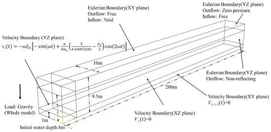
Figure 6.
Eulerian domain dimensions and boundary.
Wave generation and propagation over 60 s were simulated by explicit analysis, and the material parameters of the water are listed in Table 1. As shown in Figure 7a, the Abaqus/ODB file is redeveloped using the Python language, enabling fluid free-surface visualization. As demonstrated in Figure 7b, the simulated wave profile exhibits close agreement with theoretical Stokes second-order characteristics, validating the numerical implementation. Based on the research of Montoya [22], the meshes near the velocity boundary region, the wave generation region, and the region near the bottom of the Euler body should be encrypted and the grid size should be consistent with that shown in Figure 8 and Table 2 to ensure the accuracy of the wave data generated.

Table 1.
Material parameters of sea ice and water.
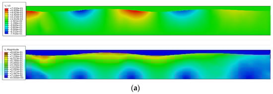
Figure 7.
Numerical simulation of wave generation. (a) Velocity distribution; (b) free surface elevation.
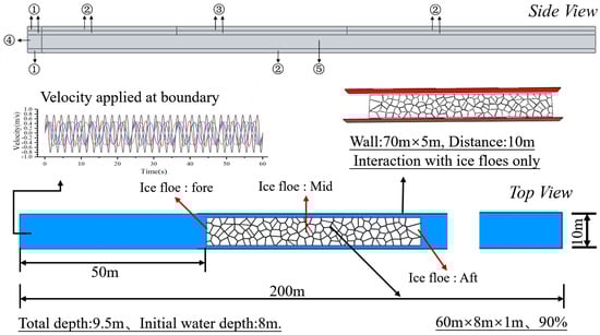
Figure 8.
Numerical modeling of wave−ice floe interaction (side view; top view).
Table 2.
Mesh sizes of Eulerian domain.
3.2. Numerical Models and Working Conditions
In this section, the CEL approach is used to study the interaction between waves and ice floes. The numerical model configuration (Figure 8) maintains consistent Eulerian domain dimensions and boundary conditions with the validated wave tank (Figure 6). Mesh size (Table 2) was determined following the study of Montoya [22], with mesh independence confirmed through systematic refinement studies, and the mesh near the velocity boundary, the area of wave generation, and the bottom region of the Euler body are appropriately encrypted. The ice floe is arranged on the left side of the Euler body, 50 m away from the boundary, and steel plates are arranged on both sides of the ice floe to restrict the movement of the ice floe in the Y direction and prevent it from escaping the Eulerian domain. The material parameters for water and sea ice are listed in Table 1.
This investigation employs numerical simulation to characterize wave–ice floe interactions, specifically examining wave propagation/attenuation through ice fields and ice floe kinematic/fracture responses under wave loading, while evaluating the influence of sea ice concentration and wave period. Three distinct ice concentration configurations were implemented: 100% concentration representing continuous level ice, alongside 90% and 70% concentrations. The numerical conditions are listed in Table 3.
Table 3.
Numerical conditions.
3.3. Analysis of Results
Initial analysis focused on ice floe kinematics and fracture dynamics under wave loading. At 90% concentration, longitudinal floe displacement exhibited phase-correlated motion with wave propagation, while vertical movement synchronized with free-surface elevation. This behavior is visualized in Figure 9a,b through displacement magnitude contour plots, where color gradients correspond to wave phase (crest/trough). Larger ice features underwent significant flexural deformation prior to fracture, as demonstrated by the bending failure sequence in Figure 9c,d. In contrast, smaller floes exhibited no fracture due to insufficient wave-induced stresses relative to their structural capacity.
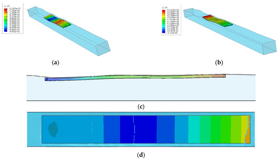
Figure 9.
Motion and fracture of ice floes under regular waves. (a) Time = 20 s, Case 6; (b) time = 30 s, Case 6; (c) ice bending, Case 7; (d) ice bending fracture, Case 7.
Three ice floes (fore, mid, and aft, as shown in Figure 8) within the ice floe field were analyzed for the multi-directional motion characteristics. During simulations, the gravity step is between 0 and 5 s, with only gravity load applied during this step, and wave step is between 5 and 60 s. As shown in Figure 10, it is worth noting that, because the initial position of the ice floe is above the water surface, the vertical displacement occurs due to the action of gravity during the simulation process, so the vertical displacement is basically less than 0 in Figure 10d. The movement of ice floes under the action of waves has obvious periodic characteristics, and the period is approximately equal to the wave period, which is consistent with the phenomenon when a wave interacts with a single ice floe. The rotational motion of the ice floe is between ±0.1 rad, and the longitudinal ice floe moves reciprocating with the waves, but, on the whole, it moves forward and, at 90% concentration, due to the small spacing between multiple ice floes, the probability of collision is larger, so the longitudinal displacement has no obvious reciprocating characteristics.
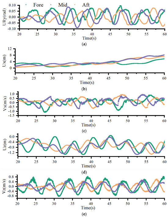
Figure 10.
The motion displacement and velocity of typical ice floes (Case 6). (a) Rotational motion; (b) longitudinal displacement; (c) longitudinal velocity; (d) vertical displacement; (e) vertical velocity.
At 70% concentration, the longitudinal motion of the ice floe shows obvious reciprocating characteristics, as shown in Figure 11a. Compared with the longitudinal displacement, the vertical displacement of ice floe is more periodic, but it is also significantly correlated with the collision between ice floes, as shown in Figure 11b, the vertical displacement at low density is more regular, and the vertical displacement amplitude is basically the same and basically consistent with the height of the wave. Comparing the vertical velocity and vertical displacement, there is also a certain phase difference between the two, as shown in Figure 11c,e, consistent with viscous damping effects in the ice–water system. Wave-induced attenuation is evident in Figure 11c, where the aft-positioned ice floe shows reduced vertical displacement amplitude, suggesting energy dissipation during wave propagation through the ice field.
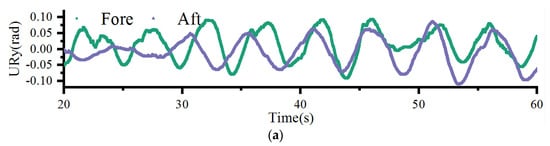
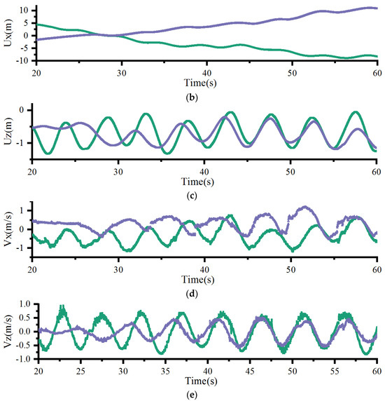
Figure 11.
The motion displacement and velocity of typical ice floes (Case 2). (a) Rotational motion; (b) longitudinal displacement; (c) vertical displacement; (d) longitudinal velocity; (e) vertical velocity.
Figure 11b traces the longitudinal displacement evolution of fore (green curve) and aft (purple curve) positioned ice floes under wave action. The fore-floe exhibits a pronounced phase opposition to the aft-floe. This anti-phase relationship suggests wave-induced differential forcing modulated by floe spacing and hydrodynamic coupling. Figure 12 provides granular insight into the collision mechanics. The longitudinal velocity of fore-floe (Vx, red curve) demonstrates pre-collision harmonic oscillations. At t = 18.3 s, Vx undergoes a discontinuous transition from 0.5 m/s to −1.0 m/s, consistent with impulsive force dynamics during floe contact. The inset illustrates contact mechanics, where stress concentration (red zones) at the floe edges aligns with velocity gradient discontinuities, validating the momentum transfer mechanism.
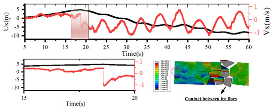
Figure 12.
The motion displacement and velocity of ice floes at fore in Case 2.
Rotational dynamics of aft-positioned ice floes across varying wave conditions (Cases 1–5) reveal distinct oscillation regimes (Figure 13). All cases show angular displacements within ±0.15 rad, with Case 4 (purple) demonstrating the largest amplitude (±0.18 rad) and Case 2 (black) the smallest (±0.08 rad). The rotational frequency aligns with wave periodicity. Notably, Case 4 exhibits a transitional regime (T = 4.75 s), where rotational motion transitions from periodic to chaotic behavior at t = 40 s and t = 50 s, suggesting incipient floe–floe contact events. Longitudinal displacement exhibits monotonic positive drift, reaching maximum at t = 60 s, indicative of persistent Stokes drift under short-period waves.
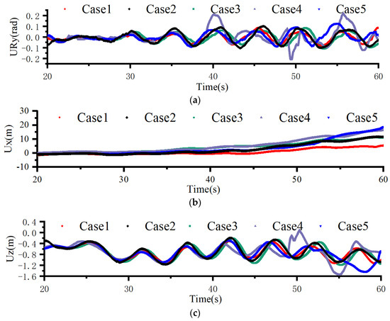
Figure 13.
The motion displacement of ice floes at aft under variable wave period and height (70% concentration ice floes). (a) Rotational motion; (b) longitudinal displacement; (c) vertical displacement.
Longitudinal ice floe displacement statistics across wave conditions (Cases 1-5) are quantified in Figure 14. From Figure 14a, it can be observed that, when the wave period is relatively short, the longitudinal displacement of the floating ice increases significantly. Figure 9b shows that, as the wave propagation distance increases, the standard deviation of the vertical displacement of the ice floe gradually decreases, suggesting that the waves attenuate as the propagation distance increases.
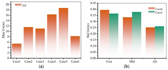
Figure 14.
Comparison of the ice floe displacements at aft of different conditions. (a) Maximum of longitudinal displacement; (b) standard deviation of longitudinal displacement.
It is obvious that the ice floe will also have a certain impact on the propagation of waves, and the conversion of wave energy into the kinetic energy of the ice floe will inevitably cause its own attenuation, as shown in Figure 15. It can be clearly seen from the figure that the wave has a significant attenuation after passing through the ice floe area. In addition, as shown in Figure 15b, the waves are strongly affected by the reflection of the level ice, and the regularity of the waves in front of the level ice gradually weakens over time.
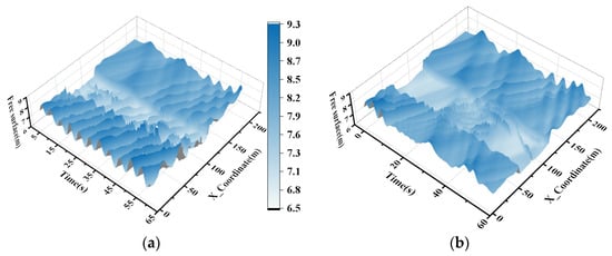
Figure 15.
Typical free surface elevation of wave passthrough ice floes. (a) Case 3; (b) Case 7.
As shown in Figure 16, the ice floe or level ice absorbs a significant amount of wave energy. The characteristics of the waves are represented by the standard deviation of the free surface height between 30 s and 60 s, with wave attenuation of more than 50% in the presence of sea ice (Case 2, Case 7 about 62%, and Case 6 about 80%). Comparing Case 2 and Case 6, it can be observed that the increase in sea ice concentration leads to an increase in the attenuation of waves. When waves pass through level ice, their attenuation is less than when passing through 90% concentration ice floes. This may be due to the boundary conditions of the level ice being fixed, not moving with the wave motion.
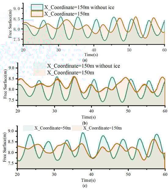
Figure 16.
Influence of ice floes on free surface of wave (70% concentration ice floes). (a) Case 2; (b) Case 7; (c) Case 6.
Figure 17 illustrates the changes in the wave free surface under different conditions with the same ice concentration. By analyzing the wave attenuation levels under the same wave height but different wave periods, it was found that the attenuation level is greater at a period T = 4.75 s at 68%, while, at T = 4.5 s, it is the lowest at 59%. This can be explained from Figure 14a, where the longitudinal displacement of the ice floe is maximized at T = 4.75 s, indicating that the ice floe absorbs more energy from the waves.
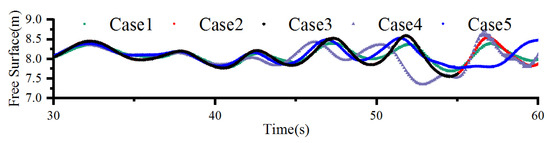
Figure 17.
Attenuation of wave passthrough ice floes.
4. Conclusions
This paper establishes a methodology for generating regular waves and random ice floes compatible with ABAQUS. Utilizing the Coupled Eulerian–Lagrangian (CEL) approach, we conduct numerical simulations of interactions between regular waves, ice floes, and level ice. The motion and fragmentation characteristics of ice floes under wave action, alongside wave attenuation through ice-covered waters, are analyzed. Key findings include:
- (1)
- Based on the velocity inlet boundary wave-generating method, a relatively ideal regular wave can be generated.
- (2)
- The ice floes move periodically in both the longitudinal and vertical directions under the action of waves, and the period is consistent with the waves, but there is a certain phase difference. The longitudinal and vertical motion characteristics of ice floe are affected by the interaction between ice floes, and the movement of ice floes under low-ice-floe concentration is more regular, and the amplitude is more consistent in different cycles.
- (3)
- The conversion of wave energy into kinetic energy of ice floe causes its own attenuation; the increase in sea ice concentration leads to an increase in the attenuation of waves.
Author Contributions
Conceptualization, Y.T. and C.Y.; methodology, C.Y.; investigation, C.Y.; data processing and analyzing, C.Y.; writing—original draft preparation, C.Y.; writing—review and editing, Y.T.; supervision.; project administration, Y.T. All authors have read and agreed to the published version of the manuscript.
Funding
This research was supported by the National Natural Science Foundation of China (Grant Nos. 52192690 and 52192693).
Data Availability Statement
The original contributions presented in this study are included in the article. Further inquiries can be directed to the corresponding author.
Conflicts of Interest
The authors declare no conflicts of interest.
References
- Li, S.; Dou, T.; Xiao, C. Research progress for the changes of Arctic Ocean surface wave with diminishing sea ice. Trans. Atmos. Sci. 2021, 44, 118–127. (In Chinese) [Google Scholar]
- Peters, A.S. The effect of a floating mat on water waves. Commun. Pure Appl. Math. 1950, 3, 319–354. [Google Scholar] [CrossRef]
- Wadhams, P. The seasonal ice zone. In The Geophysics of Sea Ice; Untersteiner, N., Ed.; Springer: Boston, MA, USA, 1986; pp. 825–991. [Google Scholar] [CrossRef]
- Luo, W.; Guo, C.; Su, Y.; Zhang, H. The study and progress of ship-wave-sea ice interaction in marginal ice zone. Shipbuild. China 2017, 58, 12–20. (In Chinese) [Google Scholar]
- Rogers, W.E.; Thomson, J.; Shen, H.H.; Doble, M.J.; Wadhams, P.; Cheng, S. Dissipation of wind waves by pancake and frazil ice in the autumn Beaufort Sea. J. Geophys. Res. Ocean. 2016, 121, 7991–8007. [Google Scholar] [CrossRef]
- Cheng, S.; Tsarau, A.; Li, H.; Herman, A.; Evers, K.U.; Shen, H. Loads on Structure and Waves in Ice (LS-WICE) project, Part 1: Wave attenuation and dispersion in broken ice fields. In Proceedings of the 24th International Conference on Port and Ocean Engineering under Arctic Conditions (POAC), Busan, Republic of Korea, 11–16 June 2017. [Google Scholar]
- Herman, A.; Tsarau, A.; Evers, K.U.; Li, H.; Shen, H. Loads on Structure and Waves in Ice (LS-WICE) project, Part 2: Sea ice breaking by waves. In Proceedings of the 24th International Conference on Port and Ocean Engineering under Arctic Conditions (POAC), Busan, Republic of Korea, 11–16 June 2017. [Google Scholar]
- Wang, C.; Wang, J.; Wang, C.; Song, M. Experimental study on longitudinal motion law of ice floes under wave action. J. Huazhong Univ. Sci. Technol. (Nat. Sci. Ed.) 2022, 50, 143–148. (In Chinese) [Google Scholar]
- Meylan, M.H. Wave response of an ice floe of arbitrary geometry. J. Geophys. Res. Ocean. 2002, 107, 5-1–5-12. [Google Scholar] [CrossRef]
- Wang, C.D.; Meylan, M.H. A higher-order-coupled boundary element and finite element method for the wave forcing of a floating elastic plate. J. Fluids Struct. 2004, 19, 557–572. [Google Scholar] [CrossRef]
- Wu, T.; Luo, W.; Jiang, D.; Deng, R.; Huang, S. Numerical study on wave-ice interaction in the marginal ice zone. J. Mar. Sci. Eng. 2020, 9, 4. [Google Scholar] [CrossRef]
- Ni, B.; Liu, C.; Hu, W.; Han, D. Numerical simulation on the interaction between two-dimensional Stokes wave and multiple ice floes. Chin. J. Hydrodyn. 2019, 34, 141–148. (In Chinese) [Google Scholar]
- Wang, C.; Wang, J.; Wang, C.; Wang, Z.; Zhang, Y. Numerical study on wave–ice floe interaction in regular waves. J. Mar. Sci. Eng. 2023, 11, 2235. [Google Scholar] [CrossRef]
- Lu, T.C.; Zou, Z.J. Numerical simulation of ice-wave interaction by coupling DEM-CFD. In Proceedings of the 38th International Conference on Ocean, Offshore and Arctic Engineering (OMAE 2019), Glasgow, UK, 9–14 June 2019; American Society of Mechanical Engineers: New York, NY, USA, 2019; Volume 8, p. V008T07A015. [Google Scholar] [CrossRef]
- Wu, J.; Liu, L.; Ji, S. Analysis of wave attenuation and ice breaking characteristics based on DEM-SPH coupling method. Chin. J. Hydrodyn. 2023, 38, 176–186. (In Chinese) [Google Scholar]
- Zhang, N.; Ma, Q.; Zheng, X.; Yan, S. A two-way coupling method for simulating wave-induced breakup of ice floes based on SPH. Eng. Fract. Mech. 2023, 282, 109148. [Google Scholar] [CrossRef]
- He, K.; Ni, B.; Xu, X.; Wei, H.; Xue, Y. Numerical simulation on the breakup of an ice sheet induced by regular incident waves. Appl. Ocean Res. 2023, 120, 103024. [Google Scholar] [CrossRef]
- Zhang, N.; Zheng, X.; Ma, Q. Study on wave-induced kinematic responses and flexures of ice floe by smoothed particle hydrodynamics. Comput. Fluids 2019, 189, 46–59. [Google Scholar] [CrossRef]
- Ni, B.; Xiong, H.; Han, D.; Zeng, L.; Sun, L.; Tan, H. A review of ice deformation and breaking under flexural-gravity waves induced by moving loads. J. Mar. Sci. Appl. 2024; advance online publication. [Google Scholar] [CrossRef]
- Majlesi, A.; Shahriar, A.; Nasouri, R.; Montoya, A.; Du, A.; Testik, F.Y.; Matamoros, A. The evaluation of explicit parameters on Eulerian-Lagrangian simulation of wave impact on coastal bridges. Coast. Eng. 2024, 191, 104540. [Google Scholar] [CrossRef]
- Kim, D.H.; Kim, S.; Kim, S.W. Numerical analysis of drop impact-induced damage of a composite fuel tank assembly on a helicopter considering liquid sloshing. Compos. Struct. 2019, 229, 111438. [Google Scholar] [CrossRef]
- Montoya, A.; Matamoros, A.; Testik, F.; Nasouri, R.; Shahriar, A.; Majlesi, A. Structural Vulnerability of Coastal Bridges Under extreme Hurricane Conditions; Report No. 18STTSA04; Transportation Consortium of South-Central States: Kunming, China, 2019. [Google Scholar]
Disclaimer/Publisher’s Note: The statements, opinions and data contained in all publications are solely those of the individual author(s) and contributor(s) and not of MDPI and/or the editor(s). MDPI and/or the editor(s) disclaim responsibility for any injury to people or property resulting from any ideas, methods, instructions or products referred to in the content. |
© 2025 by the authors. Licensee MDPI, Basel, Switzerland. This article is an open access article distributed under the terms and conditions of the Creative Commons Attribution (CC BY) license (https://creativecommons.org/licenses/by/4.0/).