
Ice Ice Maybe: Stream Hydrology and Hydraulic Processes During a Mild Winter in a Semi-Alluvial Channel

Abstract
1. Introduction
2. Methods
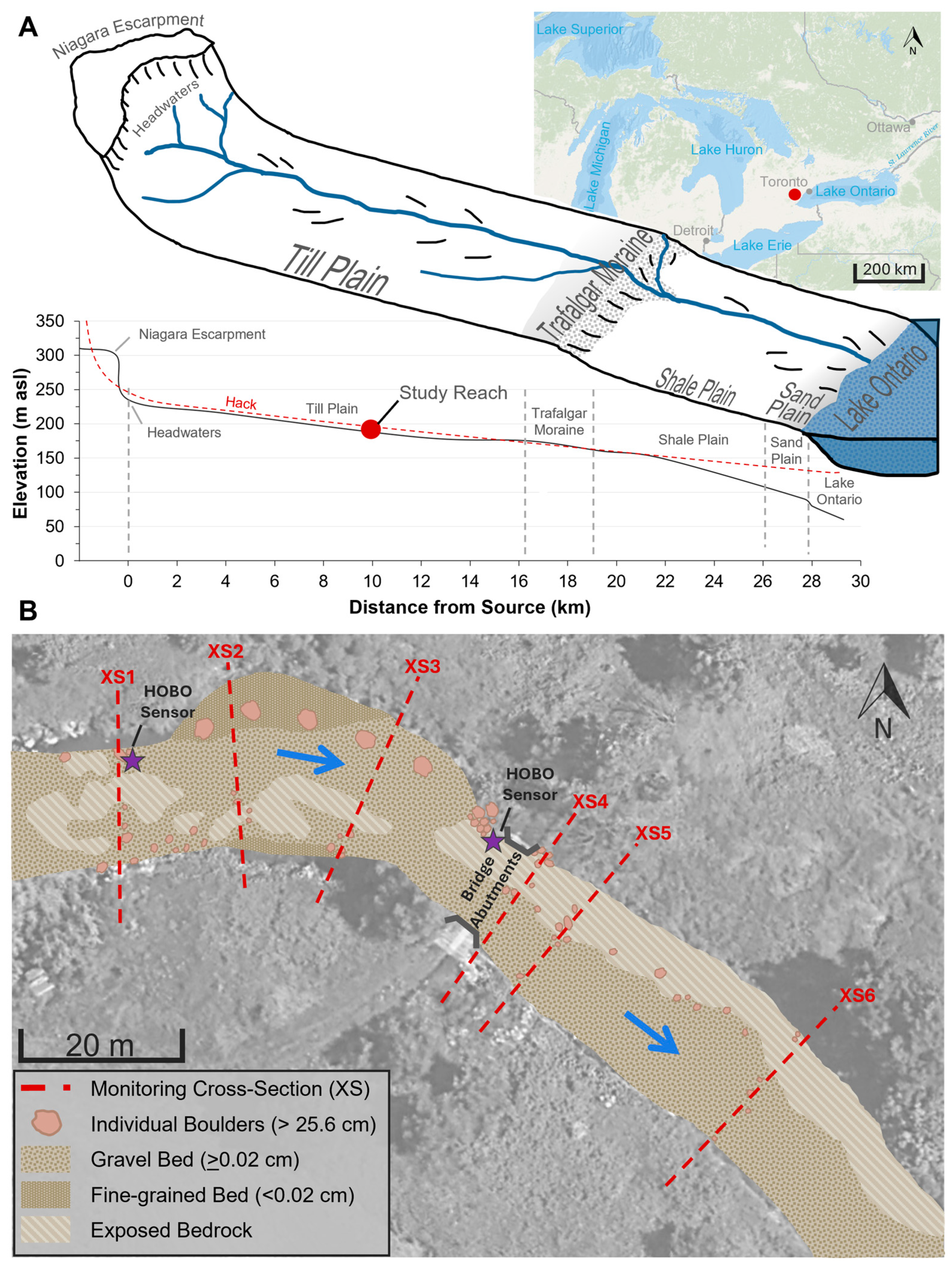
2.1. Study Reach
2.2. Field Data Collection
2.3. Data Processing and Data Analysis
3. Results
3.1. Sixteen Mile Creek Study Reach Field Conditions
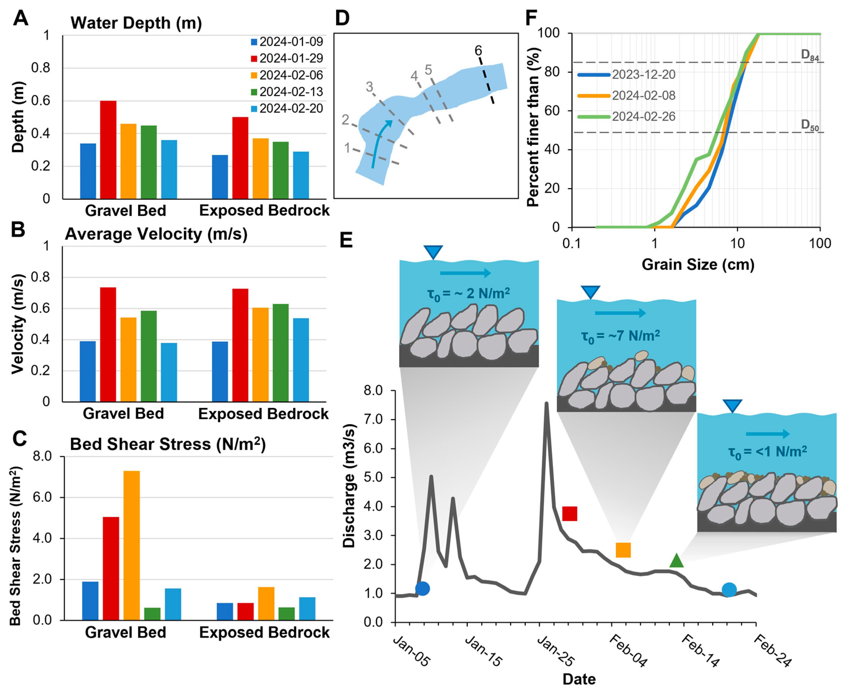
3.2. Velocity Patterns in the 2024 Field Season
3.3. Bed Shear Stress and Bed Type
4. Discussion
Mild Winter Flow Regimes Impact Local Bed Hydraulics
5. Conclusions
Supplementary Materials
Author Contributions
Funding
Data Availability Statement
Acknowledgments
Conflicts of Interest
Abbreviations
| ROS | Rain-on-snow |
| RTK-GPS | Real-Time Kinematic Global Positioning System |
| ADV | Acoustic Döppler Velocimeter |
| XS | Cross-section |
References
- Kämäri, M.; Alho, P.; Veijalainen, N.; Aaltonen, J.; Huokuna, M.; Lotsari, E. River Ice Cover Influence on Sediment Transportation at Present and under Projected Hydroclimatic Conditions. Hydrol. Process. 2015, 29, 4738–4755. [Google Scholar] [CrossRef]
- Thellman, A.; Jankowski, K.J.; Hayden, B.; Yang, X.; Dolan, W.; Smits, A.P.; O’Sullivan, A.M. The Ecology of River Ice. J. Geophys. Res. Biogeosci. 2021, 126, e2021JG006275. [Google Scholar] [CrossRef]
- Lindenschmidt, K.-E.; Baulch, H.M.; Cavaliere, E. River and Lake Ice Processes—Impacts of Freshwater Ice on Aquatic Ecosystems in a Changing Globe. Water 2018, 10, 1586. [Google Scholar] [CrossRef]
- Beltaos, S.; Burrell, B.C. Effects of River-Ice Breakup on Sediment Transport and Implications to Stream Environments: A Review. Water 2021, 13, 2541. [Google Scholar] [CrossRef]
- Lotsari, E.; Lintunen, K.; Kasvi, E.; Alho, P.; Blåfield, L. The Impacts of Near-Bed Flow Characteristics on River Bed Sediment Transport under Ice-Covered Conditions in 2016–2021. J. Hydrol. 2022, 615, 128610. [Google Scholar] [CrossRef]
- Powell, D.M. Flow Resistance in Gravel-Bed Rivers: Progress in Research. Earth-Sci. Rev. 2014, 136, 301–338. [Google Scholar] [CrossRef]
- Smith, K.; Cockburn, J.; Villard, P. The Effect of Ice Cover on Velocity and Shear Stress in a Riffle-pool Sequence. Earth Surf. Process. Landf. 2023, 48, 1414–1427. [Google Scholar] [CrossRef]
- IPCC. Climate Change 2021—The Physical Science Basis: Working Group I Contribution to the Sixth Assessment Report of the Intergovernmental Panel on Climate Change, 1st ed.; Cambridge University Press: Cambridge, UK, 2023; ISBN 978-1-00-915789-6. [Google Scholar]
- Anderson, C.I.; Gough, W.A. Evolution of Winter Temperature in Toronto, Ontario, Canada: A Case Study of Winters 2013/14 and 2014/15. J. Clim. 2017, 30, 5361–5376. [Google Scholar] [CrossRef]
- Barnett, T.P.; Adam, J.C.; Lettenmaier, D.P. Potential Impacts of a Warming Climate on Water Availability in Snow-Dominated Regions. Nature 2005, 438, 303–309. [Google Scholar] [CrossRef]
- Champagne, O.; Arain, M.A.; Leduc, M.; Coulibaly, P.; McKenzie, S. Future Shift in Winter Streamflow Modulated by the Internal Variability of Climate in Southern Ontario. Hydrol. Earth Syst. Sci. 2020, 24, 3077–3096. [Google Scholar] [CrossRef]
- Deng, Z.; Qiu, X.; Liu, J.; Madras, N.; Wang, X.; Zhu, H. Trend in Frequency of Extreme Precipitation Events over Ontario from Ensembles of Multiple GCMs. Clim. Dyn. 2016, 46, 2909–2921. [Google Scholar] [CrossRef]
- Suriano, Z.J. North American Rain-on-Snow Ablation Climatology. Clim. Res. 2022, 87, 133–145. [Google Scholar] [CrossRef]
- Myers, D.T.; Ficklin, D.L.; Robeson, S.M. Hydrologic Implications of Projected Changes in Rain-on-Snow Melt for Great Lakes Basin Watersheds. Hydrol. Earth Syst. Sci. 2023, 27, 1755–1770. [Google Scholar] [CrossRef]
- Beltaos, S.; Prowse, T. River-Ice Hydrology in a Shrinking Cryosphere. Hydrol. Process. 2009, 23, 122–144. [Google Scholar] [CrossRef]
- Mao, L. The Effect of Hydrographs on Bed Load Transport and Bed Sediment Spatial Arrangement. J. Geophys. Res. Earth Surf. 2012, 117, F03024. [Google Scholar] [CrossRef]
- Perret, E.; Berni, C.; Camenen, B.; Herrero, A.; El Kadi Abderrezzak, K. Transport of Moderately Sorted Gravel at Low Bed Shear Stresses: The Role of Fine Sediment Infiltration. Earth Surf. Process. Landf. 2018, 43, 1416–1430. [Google Scholar] [CrossRef]
- Khuntia, J.R.; Devi, K.; Proust, S.; Khatua, K.K. Depth-Averaged Velocity and Bed Shear Stress in Unsteady Open Channel Flow over Rough Bed. E3S Web Conf. 2018, 40, 05071. [Google Scholar] [CrossRef]
- Mason, R.J.; Polvi, L.E. Unravelling Fluvial versus Glacial Legacy Controls on Boulder-Bed River Geomorphology for Semi-Alluvial Rivers in Fennoscandia. Earth Surf. Process. Landf. 2023, 48, 2900–2919. [Google Scholar] [CrossRef]
- Polvi, L.E.; Lind, L.; Persson, H.; Miranda-Melo, A.; Pilotto, F.; Su, X.; Nilsson, C. Facets and Scales in River Restoration: Nestedness and Interdependence of Hydrological, Geomorphic, Ecological, and Biogeochemical Processes. J. Environ. Manag. 2020, 265, 110288. [Google Scholar] [CrossRef]
- Chaitanya, J.C.; Patel, P.L. Experimental Investigation of Turbulent Flow Velocity Distribution Profile and Bed Shear Stress over Alluvial Beds. In World Environmental and Water Resources Congress 2024; American Society of Civil Engineers: Reston, VA, USA, 2024; pp. 702–715. [Google Scholar]
- Rathore, V.; Penna, N.; Dey, S.; Gaudio, R. Response of Open-Channel Flow to a Sudden Change from Smooth to Rough Bed. Environ. Fluid Mech. 2022, 22, 87–112. [Google Scholar] [CrossRef]
- Bergman, N.; Van De Wiel, M.J.; Hicock, S.R. Sedimentary Characteristics and Morphologic Change of Till-Bedded Semi-Alluvial Streams: Medway Creek, Southern Ontario, Canada. Geomorphology 2022, 399, 108061. [Google Scholar] [CrossRef]
- Church, M.; Ferguson, R.I. Morphodynamics: Rivers Beyond Steady State. Water Resour. Res. 2015, 51, 1883–1897. [Google Scholar] [CrossRef]
- Rhoads, B.L. River Dynamics: Geomorphology to Support Management; Cambridge University Press: Cambridge, UK, 2020; ISBN 978-1-107-19542-4. [Google Scholar]
- Bevan, V.; MacVicar, B.; Chapuis, M.; Ghunowa, K.; Papangelakis, E.; Parish, J.; Snodgrass, W. Enlargement and Evolution of a Semi-Alluvial Creek in Response to Urbanization. Earth Surf. Process. Landf. 2018, 43, 2295–2312. [Google Scholar] [CrossRef]
- Ferguson, S.P.; Rennie, C.D. Influence of Alluvial Cover and Lithology on the Adjustment Characteristics of Semi-Alluvial Bedrock Channels. Geomorphology 2017, 285, 260–271. [Google Scholar] [CrossRef]
- Phillips, R.T.J.; Desloges, J.R. Glacially Conditioned Specific Stream Powers in Low-Relief River Catchments of the Southern Laurentian Great Lakes. Geomorphology 2014, 206, 271–287. [Google Scholar] [CrossRef]
- Polvi, L.E. Morphodynamics of Boulder-Bed Semi-Alluvial Streams in Northern Fennoscandia: A Flume Experiment to Determine Sediment Self-Organization. Water Resour. Res. 2021, 57, e2020WR028859. [Google Scholar] [CrossRef]
- Desloges, J.R.; Phillips, R.T.J.; Byrne, M.-L.; Cockburn, J.M.H. Geomorphology of the Great Lakes Lowlands of Eastern Canada. In Landscapes and Landforms of Eastern Canada; Slaymaker, O., Catto, N., Eds.; World Geomorphological Landscapes; Springer International Publishing: Berlin/Heidelberg, Germany, 2020; pp. 259–275. ISBN 978-3-030-35137-3. [Google Scholar]
- Ontario Greenbelt Alliance. Report: Good Things Are Growing in Ontario. Available online: https://environmentaldefence.ca/report/report-good-things-are-growing-in-ontario/ (accessed on 23 June 2025).
- Papangelakis, E.; Hassan, M.A. The Role of Channel Morphology on the Mobility and Dispersion of Bed Sediment in a Small Gravel-Bed Stream. Earth Surf. Process. Landf. 2016, 41, 2191–2206. [Google Scholar] [CrossRef]
- Ontario Geological Survey. 1:250,000 Scale Bedrock Geology of Ontario; Ontario Geological Survey: Sudbury, ON, Canada, 2011. [Google Scholar]
- Sharpe, D.R.; Russell, H.A.J. A Revised Depositional Setting for Halton Sediments in the Oak Ridges Moraine Area, Ontario. Can. J. Earth Sci. 2016, 53, 281–303. [Google Scholar] [CrossRef]
- Gough, W.A.; Tam, B.Y.; Mohsin, T.; Allen, S.M.J. Extreme Cold Weather Alerts in Toronto, Ontario, Canada and the Impact of a Changing Climate. Urban Clim. 2014, 8, 21–29. [Google Scholar] [CrossRef]
- Environment and Climate Change. Canadian Climate Normals—Climate—Environment and Climate Change Canada. Available online: https://climate.weather.gc.ca/climate_normals/index_e.html (accessed on 6 January 2025).
- Environment and Climate Change. Water Survey of Canada. Available online: https://www.canada.ca/en/environment-climate-change/services/water-overview/quantity/monitoring/survey.html (accessed on 1 April 2023).
- Lotsari, E.; Kasvi, E.; Kämäri, M.; Alho, P. The Effects of Ice Cover on Flow Characteristics in a Subarctic Meandering River. Earth Surf. Process. Landf. 2017, 42, 1195–1212. [Google Scholar] [CrossRef]
- Carlson. BRx7 Manual. Available online: https://files.carlsonsw.com/mirror/manuals/Carlson%20BRx7%20manual.pdf (accessed on 15 January 2025).
- Wolman, M.G. A Method of Sampling Coarse River-Bed Material. Trans. Am. Geophys. Union 1954, 35, 951–956. [Google Scholar] [CrossRef]
- Flowtracker2-Brochure. Available online: https://www.sontek.com/media/pdfs/flowtracker2-brochure-s19-02-1219.pdf (accessed on 9 September 2021).
- Ghareh Aghaji Zare, S.; Moore, S.A.; Rennie, C.D.; Seidou, O.; Ahmari, H.; Malenchak, J. Boundary Shear Stress in an Ice-Covered River during Breakup. J. Hydraul. Eng. 2016, 142, 04015065. [Google Scholar] [CrossRef]
- Afzalimehr, H.; Rennie, C.D. Determination of Bed Shear Stress in Gravel-Bed Rivers Using Boundary-Layer Parameters. Hydrol. Sci. J. 2009, 54, 147–159. [Google Scholar] [CrossRef]
- Ting, F.C.K.; Kern, G.S. Finding the Bed Shear Stress on a Rough Bed Using the Log Law. J. Waterw. Port Coast. Ocean Eng. 2022, 148, 04022008. [Google Scholar] [CrossRef]
- Kim, D.; Kim, J.; Son, G.; Park, Y. Experimental Evaluation of Estimating Local Bed Shear Stress Using Log Law in a Straight River Channel. KSCE J. Civ. Eng. 2024, 28, 1094–1107. [Google Scholar] [CrossRef]
- Biron, P.M.; Lane, S.N.; Roy, A.G.; Bradbrook, K.F.; Richards, K.S. Sensitivity of Bed Shear Stress Estimated from Vertical Velocity Profiles: The Problem of Sampling Resolution. Earth Surf. Process. Landf. 1998, 23, 133–139. [Google Scholar] [CrossRef]
- Robert, A. River Processes: An Introduction to Fluvial Dynamics; Routledge: London, UK, 2003. [Google Scholar]
- Environment and Climate Change. Winter 2023/2024. Available online: https://www.canada.ca/content/dam/eccc/documents/pdf/climate-change/trends-variations/winter2024/CTVB_Winter_2024-Bulletin_EN.pdf (accessed on 1 April 2024).
- NOAA. Historical El Nino/La Nina Episodes (1950–Present). Available online: https://origin.cpc.ncep.noaa.gov/products/analysis_monitoring/ensostuff/ONI_v5.php (accessed on 23 May 2024).
- Gleason, C.J. Hydraulic Geometry of Natural Rivers: A Review and Future Directions. Prog. Phys. Geogr. Earth Environ. 2015, 39, 337–360. [Google Scholar] [CrossRef]
- Wilcock, D.N. Investigation into the Relations between Bedload Transport and Channel Shape. GSA Bull. 1971, 82, 2159–2176. [Google Scholar] [CrossRef]
- Ahmed, S.I.; Rudra, R.; Goel, P.; Amili, A.; Dickinson, T.; Singh, K.; Khan, A. Change in Winter Precipitation Regime across Ontario, Canada. Hydrology 2022, 9, 81. [Google Scholar] [CrossRef]
- Deen, T.A.; Arain, M.A.; Champagne, O.; Chow-Fraser, P.; Martin-Hill, D. Impacts of Climate Change on Streamflow in the McKenzie Creek Watershed in the Great Lakes Region. Front. Environ. Sci. 2023, 11, 1171210. [Google Scholar] [CrossRef]
- Turcotte, B.; Morse, B. The Winter Environmental Continuum of Two Watersheds. Water 2017, 9, 337. [Google Scholar] [CrossRef]
- Jankowski, K.J.; Houser, J.N.; Scheuerell, M.D.; Smits, A.P. Warmer Winters Increase the Biomass of Phytoplankton in a Large Floodplain River. J. Geophys. Res. Biogeosci. 2021, 126, e2020JG006135. [Google Scholar] [CrossRef]
- Hassan, M.A.; Radić, V.; Buckrell, E.; Chartrand, S.M.; McDowell, C. Pool-Riffle Adjustment Due to Changes in Flow and Sediment Supply. Water Resour. Res. 2021, 57, e2020WR028048. [Google Scholar] [CrossRef]
- Grillakis, M.G.; Koutroulis, A.G.; Tsanis, I.K. Climate Change Impact on the Hydrology of Spencer Creek Watershed in Southern Ontario, Canada. J. Hydrol. 2011, 409, 1–19. [Google Scholar] [CrossRef]
- Nalley, D.; Adamowski, J.; Biswas, A.; Gharabaghi, B.; Hu, W. A Multiscale and Multivariate Analysis of Precipitation and Streamflow Variability in Relation to ENSO, NAO and PDO. J. Hydrol. 2019, 574, 288–307. [Google Scholar] [CrossRef]
- Walsh, C.R.; Patterson, R.T. Precipitation and Temperature Trends and Cycles Derived from Historical 1890–2019 Weather Data for the City of Ottawa, Ontario, Canada. Environments 2022, 9, 35. [Google Scholar] [CrossRef]
- Cohen, J.; Ye, H.; Jones, J. Trends and Variability in Rain-on-Snow Events. Geophys. Res. Lett. 2015, 42, 7115–7122. [Google Scholar] [CrossRef]
- Il Jeong, D.; Sushama, L. Rain-on-Snow Events over North America Based on Two Canadian Regional Climate Models. Clim. Dyn. 2018, 50, 303–316. [Google Scholar] [CrossRef]
- Reid, D.E.; Hickin, E.J.; Babakaiff, S.C. Low-Flow Hydraulic Geometry of Small, Steep Mountain Streams in Southwest British Columbia. Geomorphology 2010, 122, 39–55. [Google Scholar] [CrossRef]
- Koyuncu, B.; Le, T.B. On the Impacts of Ice Cover on Flow Profiles in a Bend. Water Resour. Res. 2022, 58, e2021WR031742. [Google Scholar] [CrossRef]
- Wang, J.; Sui, J.; Karney, B.W. Incipient Motion of Non-Cohesive Sediment under Ice Cover—An Experimental Study. J. Hydrodyn. 2008, 20, 117–124. [Google Scholar] [CrossRef]
- Vetter, T. Riffle-Pool Morphometry and Stage-Dependant Morphodynamics of a Large Floodplain River (Vereinigte Mulde, Sachsen-Anhalt, Germany). Earth Surf. Process. Landf. 2011, 36, 1647–1657. [Google Scholar] [CrossRef]
- Robert, A. Characteristics of Velocity Profiles along Riffle-Pool Sequences and Estimates of Bed Shear Stress. Geomorphology 1997, 19, 89–98. [Google Scholar] [CrossRef]
- Maturana, O.; Tonina, D.; McKean, J.A.; Buffington, J.M.; Luce, C.H.; Caamaño, D. Modeling the Effects of Pulsed versus Chronic Sand Inputs on Salmonid Spawning Habitat in a Low-Gradient Gravel-Bed River. Earth Surf. Process. Landf. 2014, 39, 877–889. [Google Scholar] [CrossRef]
- Leopold, L.B.; Maddock, T. The Hydraulic Geometry of Stream Channels and Some Physiographic Implications; USGS Professional Paper; U.S. Government Printing Office: Washington, DC, USA, 1953; pp. 1–57. [Google Scholar]
- Brierley, G.; Fryirs, K.; Reid, H.; Williams, R. The dark art of interpretation in geomorphology. Geomorphology 2021, 390, 107870. [Google Scholar] [CrossRef]
- Houser, C.; Lehner, J.; Smith, A. The Field Geomorphologist in a Time of Artificial Intelligence and Machine Learning. Ann. Am. Assoc. Geogr. 2022, 112, 1260–1277. [Google Scholar] [CrossRef]


| Date (Air Temperature *) | Instruments and Methods | Notes |
|---|---|---|
| 20 December 2023 (0 °C) | ADV, RTK, PC | HOBO loggers installed, reach and XS’s surveyed |
| 9 January 2024 (3 °C) | ADV, RTK | Resistance-depth surveys along XS’s |
| 21/22 January 2024 (−3 °C) | ADV, RTK | Ice-extent survey, Minor ice jamming US of XS1 |
| 29 January 2024 (2 °C) | ADV | High flow, following rainfall |
| 6 February 2024 (2 °C) | ADV, RTK | Resistance-depth surveys along XS’s |
| 8 February 2024 (3 °C) | PC + Facies maps | Pebble counts for XS 5 and 6 |
| 13 February 2024 (4 °C) | RTK | Survey large boulders and bedrock extent |
| 20 February 2024 (2 °C) | ADV | Thin border ice at XS 2 and 3 (melted) |
| 26 February 2024 (4 °C) | PC, Facies maps | Minor biofilm growth on larger grains (>5 cm) in the downstream portion of the reach |
| 29 February 2024 (−2 °C) | ADV, Facies maps | Minor biofilm growth on larger grains (>5 cm) in the downstream portion of the reach |
| 28 March 2024 (9 °C) | ADV, PC, Facies maps | Minor biofilm growth in the downstream portion of the reach |
| 22 April 2024 (10 °C) | ADV, PC, Facies maps | Minor biofilm growth throughout the reach |
| 14 May 2024 (20 °C) | ADV, PC, Facies maps | Biofilm/Algae throughout reach, Patches of grassy vegetation in low velocity areas |
| Flow Condition | Discharge Range (m3/s) | Date (* Calculated Discharge [m3/s]) | Symbol |
|---|---|---|---|
| High Flow | ≥2.4 | 29 January 2024 (3.70) |  |
| 6 February 2024 (2.40) |  | ||
| Moderate Flow | 1.59–2.09 | 13 February 2024 (2.09) |  |
| 22 April 2024 (2.06) |  | ||
| 29 February 2024 (1.59) |  | ||
| Low Flow | ≤1.12 | 14 May 2024 (1.12) |  |
| 9 January 2024 (1.06) |  | ||
| 20 February 2024 (1.06) |  | ||
| 28 March 2024 (0.92) |  |
Disclaimer/Publisher’s Note: The statements, opinions and data contained in all publications are solely those of the individual author(s) and contributor(s) and not of MDPI and/or the editor(s). MDPI and/or the editor(s) disclaim responsibility for any injury to people or property resulting from any ideas, methods, instructions or products referred to in the content. |
© 2025 by the authors. Licensee MDPI, Basel, Switzerland. This article is an open access article distributed under the terms and conditions of the Creative Commons Attribution (CC BY) license (https://creativecommons.org/licenses/by/4.0/).
Share and Cite
Giovino, C.; Cockburn, J.M.H.; Villard, P.V. Ice Ice Maybe: Stream Hydrology and Hydraulic Processes During a Mild Winter in a Semi-Alluvial Channel. Water 2025, 17, 1878. https://doi.org/10.3390/w17131878
Giovino C, Cockburn JMH, Villard PV. Ice Ice Maybe: Stream Hydrology and Hydraulic Processes During a Mild Winter in a Semi-Alluvial Channel. Water. 2025; 17(13):1878. https://doi.org/10.3390/w17131878
Chicago/Turabian StyleGiovino, Christopher, Jaclyn M. H. Cockburn, and Paul V. Villard. 2025. "Ice Ice Maybe: Stream Hydrology and Hydraulic Processes During a Mild Winter in a Semi-Alluvial Channel" Water 17, no. 13: 1878. https://doi.org/10.3390/w17131878
APA StyleGiovino, C., Cockburn, J. M. H., & Villard, P. V. (2025). Ice Ice Maybe: Stream Hydrology and Hydraulic Processes During a Mild Winter in a Semi-Alluvial Channel. Water, 17(13), 1878. https://doi.org/10.3390/w17131878