Predictive Analytics and Soft Computing Models for Groundwater Vulnerability Assessment in High-Salinity Regions of the Southeastern Anatolia Project (GAP), Türkiye

Abstract

This study was conducted in the Harran Plain within the framework of the Southeastern Anatolia Project (GAP) in Türkiye to evaluate the vulnerability of groundwater to contamination, with a special emphasis on the high salinity conditions attributed to agricultural and rural practices. The region is notably challenged by salinization resulting from intensive irrigation and insufficient drainage systems. The DRASTIC framework was used to assess groundwater contamination vulnerability. The DRASTIC framework parameters were numerically integrated using both the original DRASTIC framework and its modified version, serving as the basis for subsequent predictive analytics and soft computing model development. The primary aim was to determine the most effective predictive model for groundwater contamination vulnerability in salinity-affected areas. In this context, various models were implemented and evaluated, including artificial neural networks (ANNs) with varied hidden layer configurations, four different regression-based methods (MARS, TreeNet, GPS, and CART), and three classical regression analysis approaches. The modeling process utilized 24 adjusted vulnerability indices (AVIs) as target variables, with the dataset partitioned into 58.34% for training, 20.83% for validating, and 20.83% for testing. Model performance was rigorously assessed using various statistical indicators such as mean absolute error, root mean square error, and the Nash–Sutcliffe efficiency coefficient, in addition to evaluating the predictive AVIs through spatial mapping. The findings revealed that the ANNs and TreeNet models offered superior performance in accurately predicting groundwater contamination vulnerability, particularly by delineating the spatial distribution of risk in areas experiencing intensive agricultural pressure.

1. Introduction

Groundwater is widely used for domestic, agricultural, and industrial purposes. It is essential for domestic use because surface water is susceptible to contamination by agricultural pollutants [1]. However, changes in precipitation regime due to climate change, reduction in groundwater recharge, urbanization, population growth, and increases in agricultural and industrial activities negatively affect the quality of groundwater in the world [2]. Therefore, it is a fundamental task to assess the vulnerability to groundwater pollution to carry out an effective strategy for the management and protection of groundwater resources against pollution [3]. Recently, assessment of vulnerability to groundwater pollution has become a critical issue in many countries around the world [4].

One of the widely used models for assessing the vulnerability of groundwater to potential pollutants is the DRASTIC framework [5,6,7,8]. The mapping of groundwater vulnerability is based on the idea that some land areas are more vulnerable to groundwater pollution than others [8]. The concept of vulnerability is to classify groundwater pollution of a geographical area according to vulnerability, rather than using dynamic groundwater models. Because groundwater models often have data requirements that cannot be met in many parts of the world [7,9]. The DRASTIC framework is a numerical rating scheme developed by the United States Environmental Protection Agency (US EPA) to assess the groundwater pollution potential in each region given its hydrogeological environment. The DRASTIC framework was used to assess groundwater contamination vulnerability, with eight hydrogeological parameters being quantified for this purpose: depth to water table (D), net recharge (R), aquifer media (A), soil media (S), topography or slope (T), impact of the vadose zone (I), and hydraulic conductivity (C).

Indexes such as DRASTIC, which are frequently used in groundwater pollution risk assessments, contain uncertainty due to subjective judgments in parameter weights. In order to reduce this uncertainty, the integration of artificial intelligence and multi-criteria methods has been proposed. For example, Sadeghfam et al. [10] developed a membership function approach based on multi-objective catastrophe theory to determine DRASTIC parameter weights according to local conditions. This method significantly increased the correlation between the adjusted DRASTIC index and measured NO₃-N concentrations. Sadeghfam et al. [11] aimed to reduce subjectivity in groundwater vulnerability assessments based on the DRASTIC framework, convert vulnerability indices into risk indices, and analyze model uncertainties. As a method, catastrophe theory and fuzzy logic were applied together to determine parameter weights according to regional conditions; then, the generalized likelihood uncertainty estimation (GLUE) approach was used for uncertainty analysis. The findings showed that the fuzzy–catastrophic approach increased the model accuracy, and the GLUE method revealed lower uncertainty levels in high-vulnerability areas and higher uncertainty levels in low-vulnerability areas. Similarly, Fijani et al. [12] developed a supervised committee machine with artificial intelligence (SCMAI) method combining four different artificial intelligence models to improve the fragility index based on DRASTIC. SCMAI showed superior performance compared to single models and provided more reliable mapping by preventing high NO₃ value wells from being incorrectly classified as minimal risk. Nadiri et al. [3,13,14] followed these studies and combined fuzzy logic and committee models. Nadiri et al. [3,13] proposed a supervised committee fuzzy logic (SCFL) framework that calculates DRASTIC parameters with three different fuzzy logic models of Sugeno, Mamdani, and Larsen types and combines these models through an artificial neural network (ANN). The vulnerability indices produced by these approaches matched the observed NO₃-N distribution much better compared to the traditional DRASTIC; the vulnerability–NO₃ correlation could be increased from approximately 0.4 to over 0.9. In a study involving multiple aquifers, fuzzy and committee-based models provided higher accuracy compared to the baseline method. Recent studies have taken this multi-method integration even further. On the other hand, Nadiri et al. [14] proposed a supervised intelligent committee machine (SICM) method that overlays support vector machines (SVM), neuro-fuzzy (NF), and gene expression programming (GEP) models with ANNs. Nadiri et al. [15,16] introduced artificial intelligence to run multiple framework (AIMF) models, which combine different DRASTIC frameworks with artificial intelligence. This model increased the correlation above 0.95 when creating vulnerability maps specific to a particular pollutant. Gharekhani et al. [17] combined ANN, GEP, and SVM models with a two-level committee using Bayesian model averaging (BMA); with this approach, maximum information was extracted from the data, and it was determined that model uncertainty was greater in high-vulnerability regions. These integrated AI multi-criteria decision-making approaches have shown that more consistent risk maps and decision support solutions can be produced by blending multi-criteria decision elements with AI-based models. Nadiri et al. [18] developed a method based on the modified traditional GALDIT framework (mod-TGF) to assess the vulnerability to seawater intrusion in the Shiramin coastal aquifer, northwest Iran. The convolutional neural network (CNN) model applied in addition to mod-TGF increased the vulnerability mapping accuracy by over 30%. This study revealed that AI-assisted approaches provide high accuracy in coastal aquifer vulnerability analyses.

Motlagh et al. [19] evaluated groundwater sensitivity using the DRASTIC framework and machine learning algorithms. Machine learning algorithms were used to optimize the DRASTIC model using the SDM package in R 4.2.2 software. It showed that 40% of the study area has a high risk of contamination, and 30% of it has a moderate risk of contamination. The random forests (RF) model achieved the highest predictive power with an AUC value of 0.98, while the generalized linear model (GLM) and support vector machine (SVM) algorithms performed at 76% AUC, respectively. Bakhtiarizadeh et al. [20] used the composite DRASTIC index and nitrate vulnerability index to evaluate the sensitivity of the Kerman–Baghin plain aquifer. In the test results, the evolutionary polynomial regression model performed the best with a correlation coefficient (R = 0.9999) and root mean square error (RMSE = 0.2105). At the same time, multivariate adaptive regression splines (MARS) classified susceptibility as very low (73.06%) and low (26.94%) in regional assessment. The findings provide effective methods for groundwater susceptibility assessment. Dasgupta et al. [21] assessed groundwater sensitivity in the North 24-Parganas region of India using the DRASTIC framework. The DRASTIC-CNN framework most effectively reduced subjectivity errors by increasing the R from 0.226 to 0.900. The findings contribute to the development of sustainable management and treatment strategies. Baki et al. [22] evaluated groundwater sensitivity by adding land use (LU) to improve the DRASTIC framework, reorganizing the weights with analytic hierarchy process (AHP), and using the TOPSIS method. Results indicate that the proposed model provides a more effective assessment. Ozegin et al. [23] assessed the groundwater contamination risk in Edo State (Nigeria) using DRASTIC, DRASTIC-AHP, and DRASTIC-L-AHP models, and different risk zones were mapped. According to the DRASTIC-L-AHP model, 45% of the region was found to be at very low risk of contamination and 25% at high risk of contamination. Sensitivity analysis showed that the vadose zone was the most effective parameter, and the model was validated by hydro-geochemical analysis and determined as a suitable tool for groundwater management. The classification and regression trees (CART) method [24] has been applied to water quality issues. Burow et al. [25] used the CART algorithm as an exploratory tool to identify factors affecting nitrate concentrations in major aquifers in the United States. The MARS method, by combining iterative partitioning and spline-based regression, models complex nonlinear relationships between input and output variables with high accuracy [26]. Due to these advantages, there is increasing interest in the use of MARS in water quality and groundwater studies [27,28].

The RF algorithms [29] have been successfully applied in modeling nitrate contamination [30]. Additionally, in a study by Uddameri et al. [31], the performance of the conventional logistic regression (LR) model used to determine the probability of exceeding nitrate threshold level for drinking water in the Ogallala Aquifer in Texas was compared with four different tree-based classification techniques (CART, MARS, RF, and GBT) to assess aquifer vulnerability. Tree-based models were found to be more flexible, better at capturing nonlinear relationships, and more reliable in predicting nitrate exceedance compared to the logistic regression (LR) model. The RF model showed the best performance in terms of both accuracy and generalization capability. Uddameri et al. [31] indicate that tree-based methods are a powerful tool for assessing aquifer vulnerability and can aid in optimizing monitoring strategies. When the studies in the literature were examined, it was observed that not all methods were used at the same time. This study provides an original contribution to the existing literature by comparatively considering ANNs, MARS, TreeNet gradient boosting machine (TreeNet), generalized path seeker (GPS), CART, and classical regression analysis (CRA).

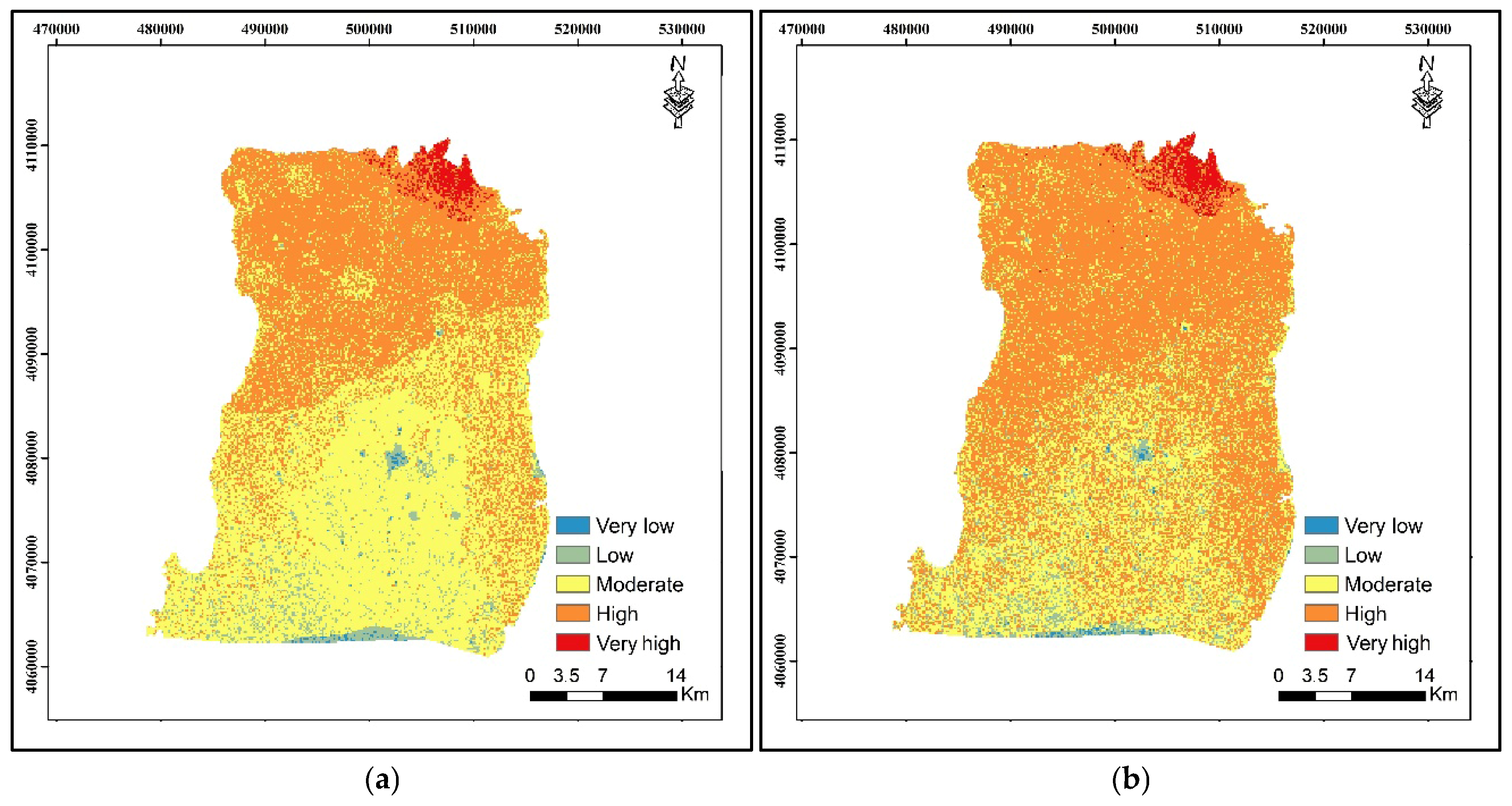
Various methods and techniques have been developed in many studies to evaluate the efficacy of the DRASTIC framework against groundwater pollution and to increase its applicability. In this study, the original DRASTIC model (ODM) and the modified DRASTIC model (MDM) were tested by adding the LU factor to determine the groundwater vulnerability of the Harran Plain using ArcGIS ArcMap 10.8, one of the geographical information system (GIS) software packages. The purpose of this study is to determine the best model among ANNs formed with different hidden layer neuron numbers and four different regression-based methods (MARS, TreeNet, GPS, and CART) applied to three functions of CRA (linear, power, and exponential) in assessing groundwater contamination vulnerability in a high groundwater salinity contaminated area. This study underscores the significance of integrating predictive models into groundwater management strategies and recommends future research to apply these methodologies to other contaminants and extend the scope to broader geographic regions.

2. Material and Methods

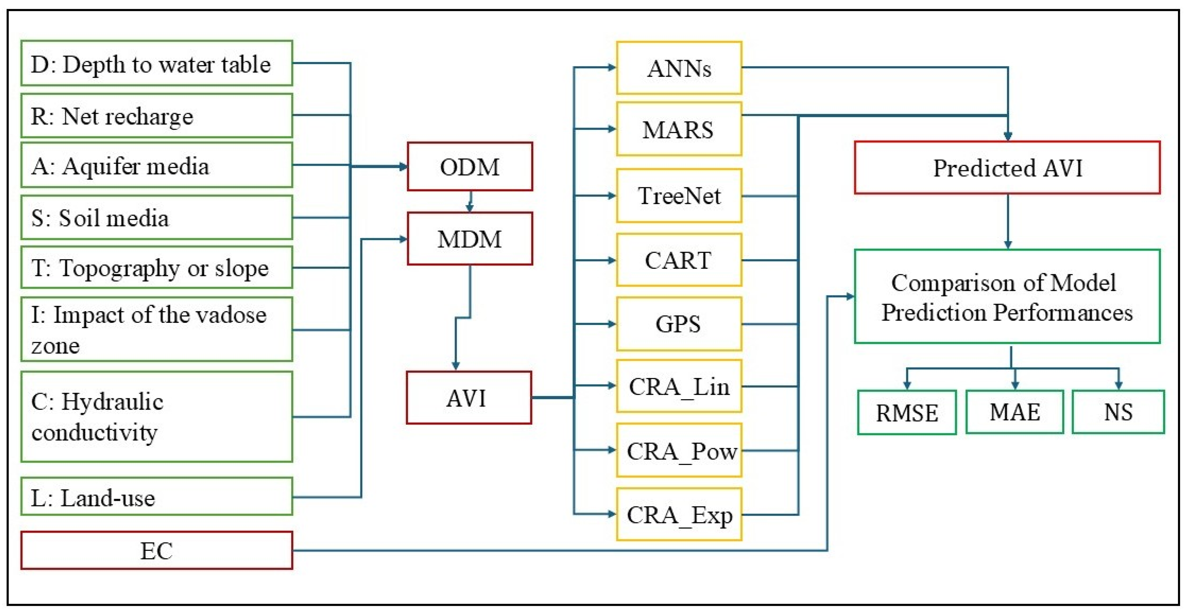
A comprehensive methodology for assessing groundwater contamination vulnerability using the DRASTIC framework is proposed in this study. The first step involves the production of thematic maps for eight hydrogeological factors that are essential in determining groundwater vulnerability. Subsequently, input factors are selected based on their predictive power, utilizing multicollinearity diagnosis through tolerance and variance inflation factor (VIF) analyses. The input data are then normalized, transforming it into dimensionless values within a range of 0 to 10 to ensure consistency and comparability across parameters. The next phase involves the calculation of the adjusted vulnerability index (AVI) as the target output, derived from the average values of the DRASTIC and electrical conductivity (EC) data. Although the DRASTIC model is based on the premise that contamination occurs primarily from surface infiltration [32], in this study, EC values are presented as general indicators of groundwater salinity, which may arise from both anthropogenic inputs (e.g., agricultural practices) and geogenic processes (e.g., rock–water interactions). It is acknowledged that certain contaminants, particularly organic or low-concentration pollutants, may not significantly alter EC values. Therefore, EC should be interpreted here as a supporting indicator rather than a direct measure of surface-derived contamination.

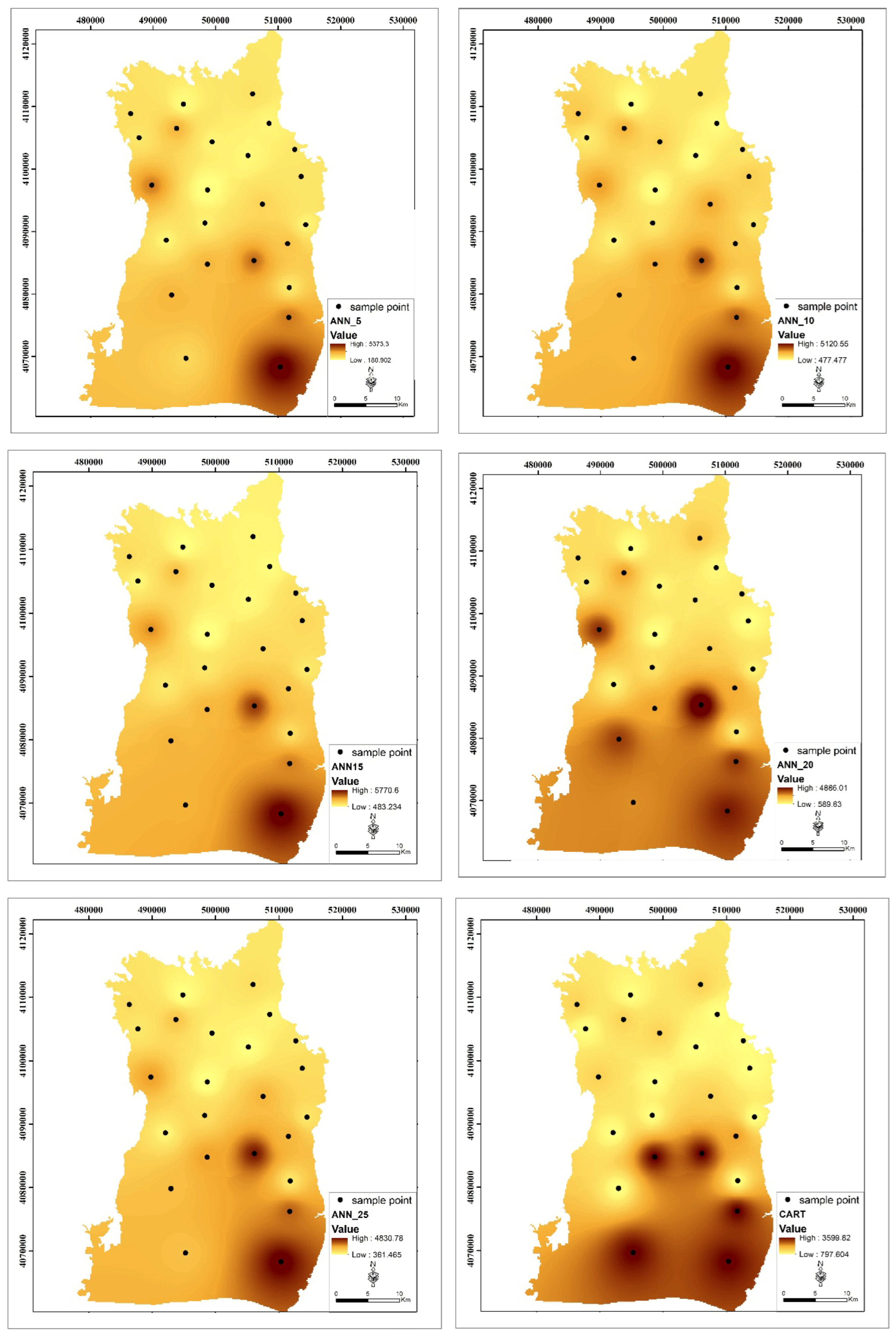
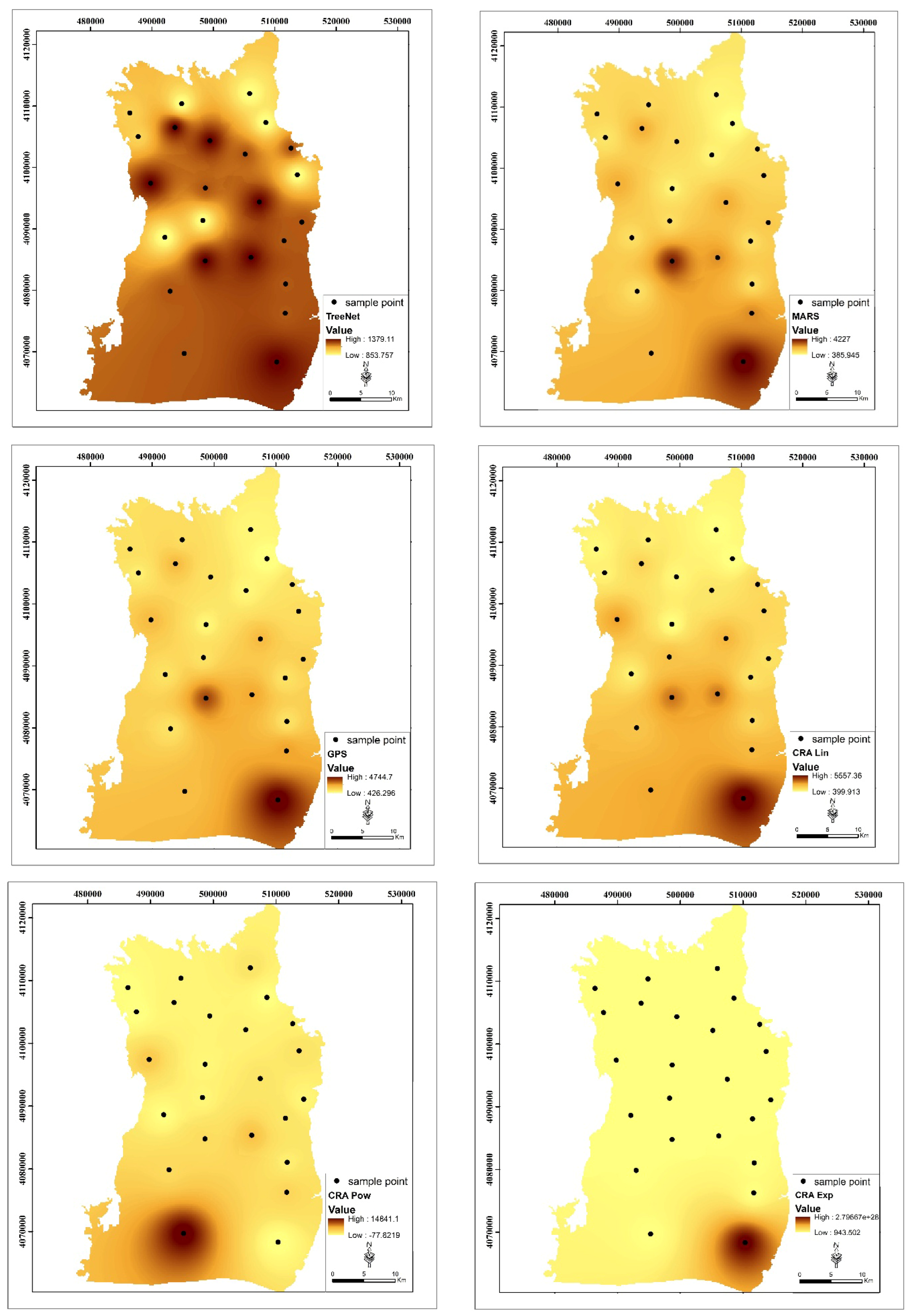
Once the input data are processed, the performance of the DRASTIC is assessed through training and testing procedures to evaluate their predictive accuracy. To further assess model performance, statistical criteria such as mean absolute error (MAE), RMSE, and Nash–Sutcliffe (NS) are employed. Additionally, the difference between the predicted AVI and the calculated AVI is analyzed to gauge model efficacy. Spatial distribution maps of the models are then generated using ArcGIS ArcMap 10.8, enabling a visual representation of groundwater vulnerability. Finally, the most accurate model is identified based on statistical evaluation criteria, including ROC/AUC curves and the R between the DRASTIC and EC values. The workflow diagram of this study is given in Figure 1.

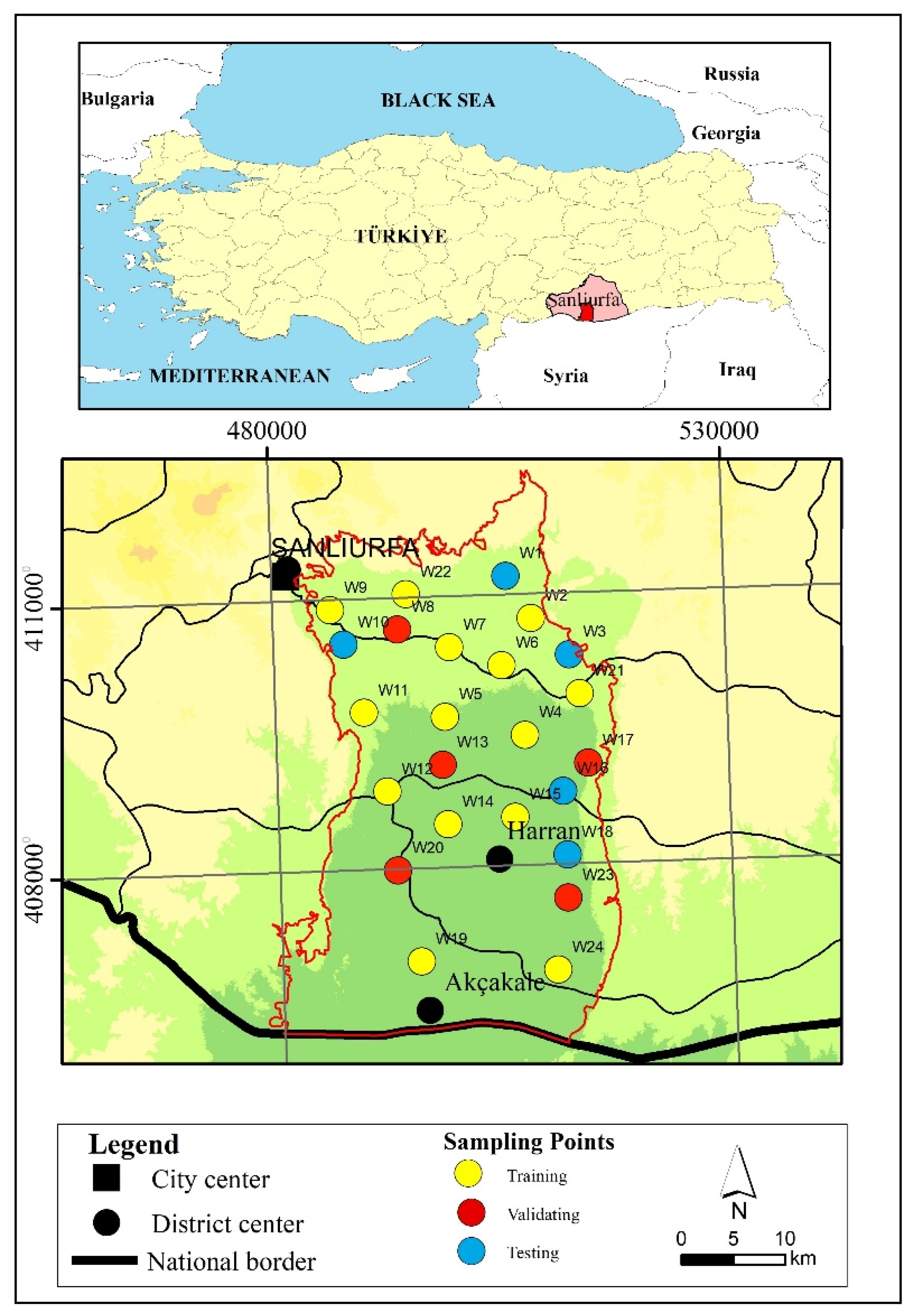
2.1. Study Area

The Harran Plain is located in the southeastern part of Türkiye and the Şanlıurfa city center. It has the largest irrigation area in the region. It is situated between latitude 36°42′–37°10′ N and longitude 38°50′–39°10′ E [33]. Considering its geomorphological borders, the approximate area of this plain is 1700 km² (

Table 1. Sample points of this study.

No	Location	X	Y	Type	Sample No	Location	X	Y	Type
W1	Camlidere	505,942.8	4,112,020	Testing	W13	Kecikiran	498,320.0	4,091,355	Validating
W2	Karabayir	508,570.0	4,107,300	Training	W14	Kizildoruc	498,715.1	4,084,765	Training
W3	Ikiagiz	512,683.9	4,103,125	Testing	W15	Yardimli	506,157.5	4,085,352	Training
W4	Vergili	507,519.8	4,094,362	Training	W16	Ozlu	511,525.1	4,088,056	Testing
W5	Yardimci	498,734.7	4,096,650	Training	W17	Olgunlar	514,431.8	4,091,080	Validating
W6	Mutluca	505,197.0	4,102,159	Training	W18	Yaygili	511,791.6	4,081,022	Testing
W7	Gunbali	499,464.6	4,104,347	Training	W19	Bolatlar	495,281.6	4,069,709	Training
W8	Kisas	493,770.7	4,106,490	Validating	W20	Ugrakli	492,980.1	4,079,844	Validating
W9	Konuklu	486,424.8	4,108,856	Training	W21	Yaşarköy	513,710.2	4,098,800	Training
W10	Hancagiz	487,778.3	4,105,003	Testing	W22	Çekçek	494,863.0	4,110,355	Training
W11	Ugurlu	489,816.2	4,097,419	Training	W23	Çepkenli	511,722.4	4,076,254	Validating
W12	Ozanlar	492,125.1	4,088,607	Training	W24	Altılı	510,345.4	4,068,335	Training

Note: Coordinate values are given with the UTM WGS 1984 37N coordinate system, units: meters.

and Figure 2). This plain has a semi-arid climate. The mean annual air temperature and precipitation depth are 18 °C and 284 mm, respectively [34].

The Harran Plain is one of the most important agricultural production areas in Türkiye and generally consists of deep-profile alluvial and residual soils. Although the soils are usually clayey in profile, their water permeability tests remain pretty good, with permeability test results showing that the permeability in the plain is generally “fast” or “very fast”. This situation accelerated the formation of groundwater and thus caused the groundwater to be vulnerable to potential pollutants. Another factor affecting the formation of the water table in the Harran Plain is the aquifer carrying groundwater. In the groundwater-bearing limestone aquifer (Eocene aquifer), despite the reported increase in water table level (free-Pleistocene aquifer), no irrigation-based effect was found [35,36]. In the first years after the start of irrigation in the Harran Plain, excessive irrigation and flood irrigation practices caused the water table to rise due to high evaporation in clay-textured soils with insufficient drainage in the lower parts of the plain. The rising water table evaporated, causing salt accumulation on the soil surface.

Within the scope of the Southeastern Anatolia Project (GAP) initiated in 1995, surface irrigation was started in the Harran Plain. Problems such as excessive irrigation and insufficient drainage, which began with surface irrigation in the plain, caused salinization. While the groundwater level was recorded as 25–30 m in 1982 in the plain, the level increased between 0 and 5 m with the start of organized irrigation in 1995 [35].

The Harran Plain, located in the southeastern part of Şanlıurfa Province, is part of the broader Euphrates River Basin and represents one of Türkiye’s most important agricultural and hydrogeological regions. Structurally, the plain is defined by a wide graben system filled with Neogene-aged alluvial and sedimentary units, including limestone, marl, clay, sand, and gravel. Coarse-grained silt, sand, and gravel materials are predominant along the plain’s margins, while finer, clay-rich deposits dominate toward the central areas. This stratigraphic variation exerts a critical influence on the spatial heterogeneity of aquifer permeability and groundwater storage dynamics. The main aquifer system consists of karstified and fractured limestones associated with the Midyat and Germav formations, exhibiting both confined and unconfined characteristics depending on localized geological settings. In addition, lens-shaped permeable units embedded within low-permeability matrices contribute to the system’s hydraulic complexity.

Groundwater in the Harran Plain generally occurs under phreatic to semi-confined conditions, with water table depths ranging from 5 to 25 m, subject to seasonal and topographic variability. Recharge mechanisms include direct precipitation, seepage from irrigation canals, and percolation from reservoirs, especially those developed under the GAP. However, intensive irrigation practices initiated after 1995, combined with inadequate drainage infrastructure, have significantly disrupted the natural recharge–discharge equilibrium. Surface irrigation methods, which are predominantly used in the region, lead to inefficient water use and an unnatural rise in groundwater levels. These conditions, exacerbated by high evaporation rates, have triggered widespread salinization, particularly in the lower elevation areas of the plain. Approximately 3000 hectares of agricultural land are currently affected by salinity, which is primarily attributed to insufficient drainage capacity and the use of low-quality irrigation water. The resulting salt accumulation in the root zone has caused notable declines in soil productivity and poses a long-term risk to sustainable agricultural development in the region.

2.2. DRASTIC Framework and Hydrogeological Factors

The concept underpinning groundwater vulnerability mapping is that certain geographical areas are more susceptible to groundwater contamination than others [8]. The vulnerability notion is instead of using dynamic groundwater models; it is applied by classifying a geographical area according to its susceptibility to groundwater pollution. Because groundwater models often have data requirements that cannot be met in many parts of the world [7,9]. DRASTIC is one of the most widely used models for assessing the vulnerability of groundwater to potential contaminants [5,6,7,8]. In this model, spatial datasets on depth to groundwater, recharge by rainfall, aquifer type, soil properties, topography, impact of the vadose zone, and the hydraulic conductivity of the aquifer are combined [9,37]. DRASTIC is a numerical rating scheme, which was developed by the US EPA, for evaluating the potential for groundwater contamination at a specific site given its hydrogeological setting [7]. Determination of the DRASTIC index involves multiplying each factor weight by its point rating and summing the total [7,9].

The ODM developed by Aller et al. [32] uses seven factors, such as depth to water, net recharge, aquifer media, soil media, topography, impact of vadose zone, and hydraulic conductivity [8,9,38,39,40]. The ODM is simple and easy to implement, but it has difficulties in correctly assessing groundwater contamination vulnerability due to subjective assessment and a few factors [4]. The weights for seven factors are as follows: depth to water: 5, net recharge: 4, aquifer media: 3, soil media: 2, topographic slope: 1, impact of vadose zone: 5, and hydraulic conductivity: 3. In addition, land use is an influencing factor in groundwater contamination vulnerability. In this study, land use is added to ODM and is assigned the weight of 5. The following equation can calculate the vulnerability index (MDVI) of ODM and MDM:

$$\begin{array}{ll}\mathrm{Modified} \mathrm{DRASTIC}& \mathrm{vulnerability} \mathrm{Index}\\ & =\mathrm{DrDw}+\mathrm{RrRw}+\mathrm{ArAw}+\mathrm{SrSw}+\mathrm{TrTw}+\mathrm{IrIw}+\mathrm{CrCw}\\ & +\mathrm{LrLw}\end{array}$$

(1)

where D is the depth to groundwater; R is the recharge rate; A is the aquifer media; S is the soil media; T represents topography (slope); I is the impact of the vadose zone; C is the hydraulic conductivity of an aquifer; L is land use; r is a rating value assigned to each factor; and w is the weight assigned to each factor.

2.3. Data for Models

2.3.1. Input Data

The ODM and MDVI have been applied for the Harran Plain unconfined aquifer, and the EC data from 24 wells in the field of study have been evaluated. The location of the sampling wells is shown in Figure 2. For the land-use factor [33], the landscape was classified using Landsat 8 OLI satellite data for 2021, as provided by the United States Geological Survey (USGS).

DRASTIC spatial distribution maps were created for the study area using the ArcGIS ArcMap 10.8. GIS is used to generate analysis and store various spatial data. Today, with increased availability of geographic data and advances in computing technology, GIS is widely used for groundwater and water resources management [41]. Overlay analysis and weighted sum analysis are frequently used for the production of groundwater vulnerability maps [42,43,44].

In this study, the standard DRASTIC parameter weights defined by Aller et al. [32] were applied uniformly across the study area without local modification. This decision was based on the relative hydrogeological homogeneity of the Harran Plain, where the aquifer media and vadose zone are predominantly composed of karstified and fractured limestone formations. However, while the parameter weights were kept constant, the rating values assigned to each thematic layer were adapted using locally obtained geological, lithological, and hydrological data. These localized ratings allowed the model to reflect spatial variation in environmental conditions even under a standardized weighting framework.

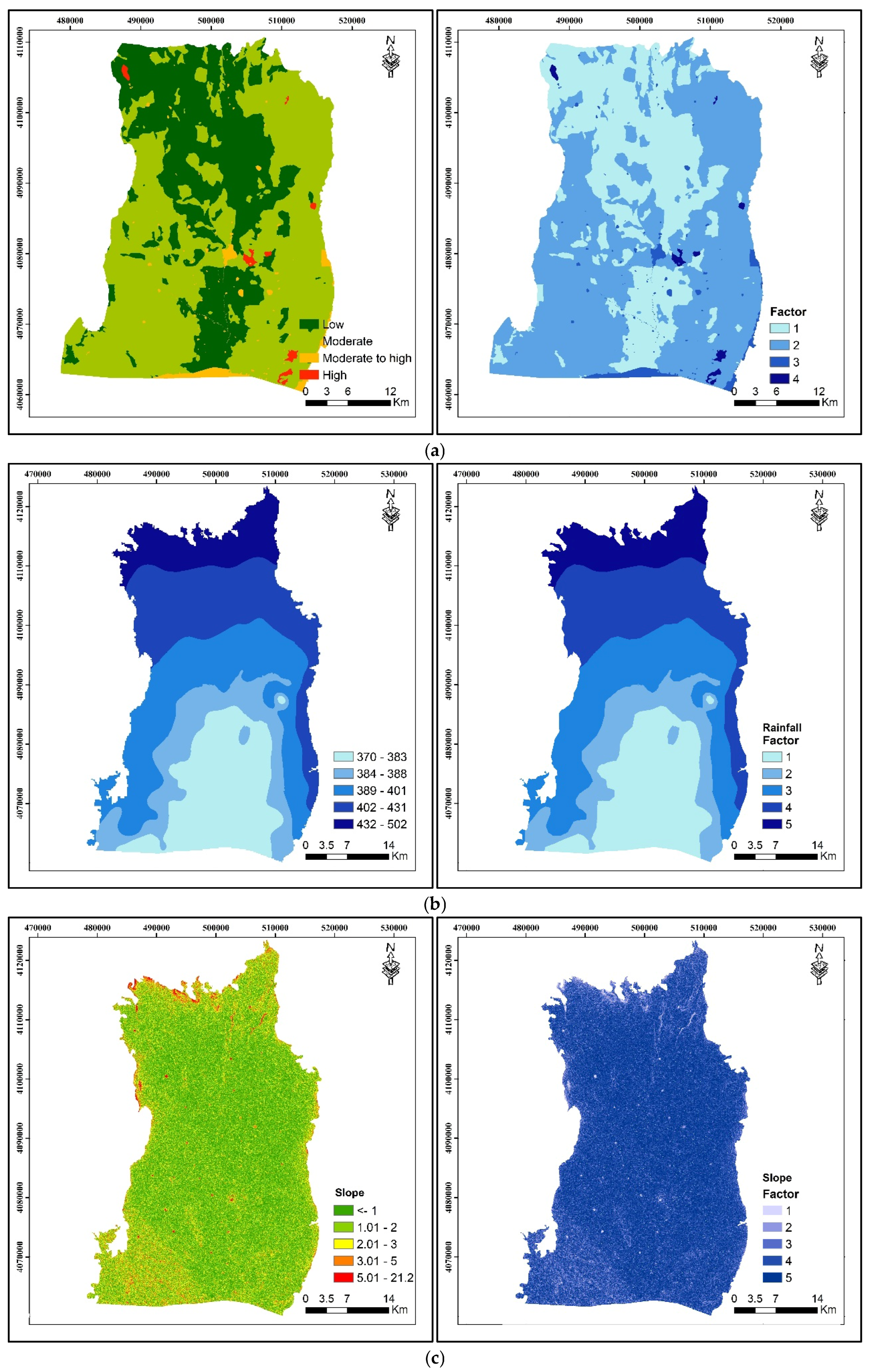
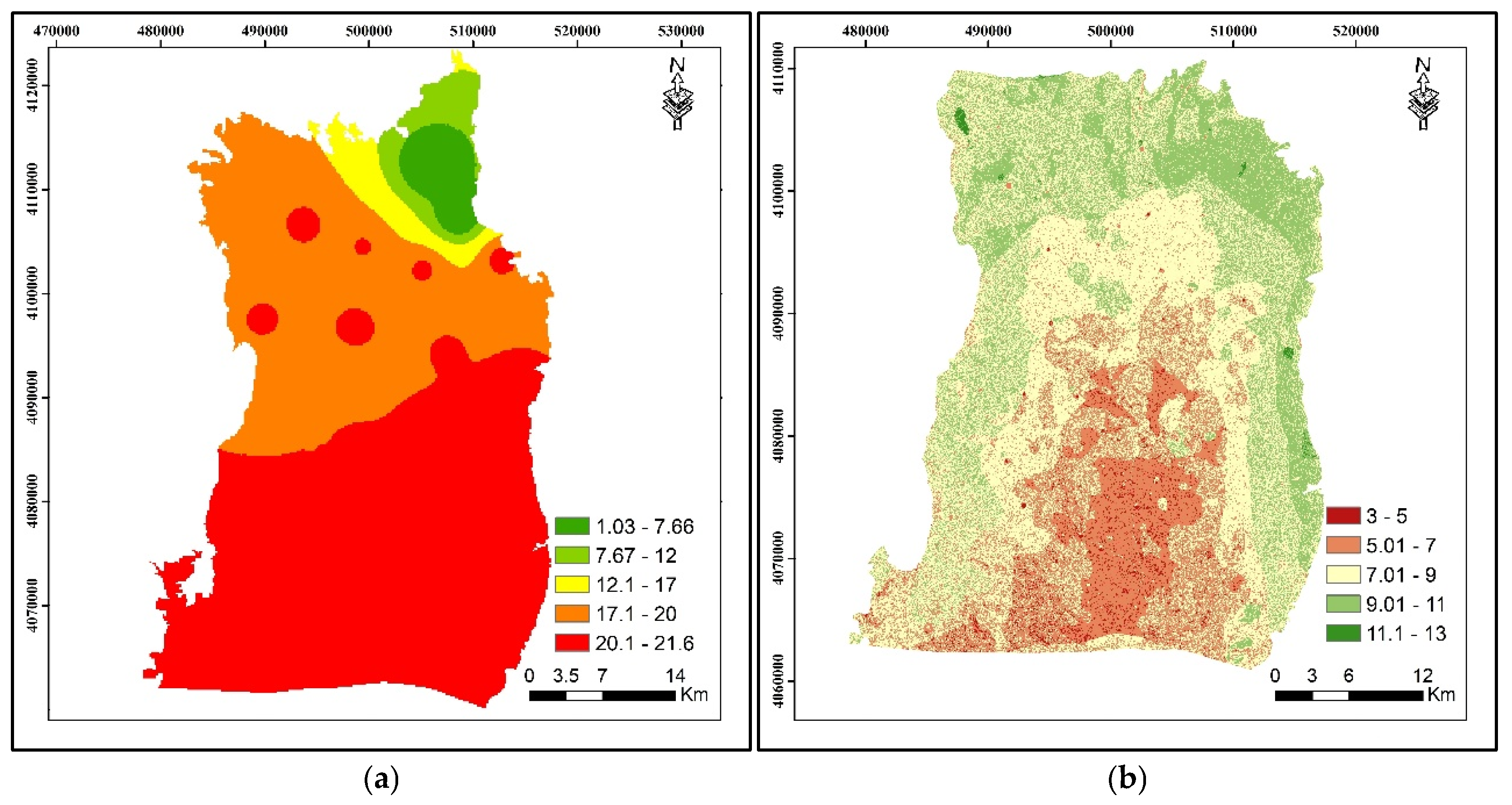
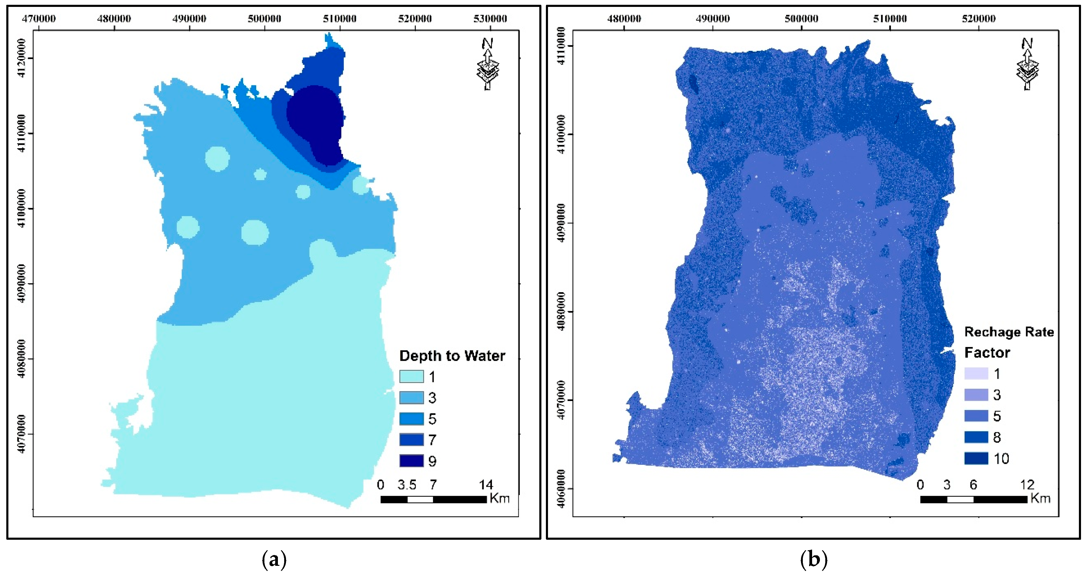
Depth to water level (m) spatial distribution maps were produced using the radial basis functions interpolation method. The maximum and minimum water level depths measured in the watershed are 20.80 m and 1.03 m below ground level, respectively. This point data were divided into five classes. Recharge rate is the amount of water that penetrates the ground surface and reaches the water table; recharge water represents the medium for transporting pollutants [40]. For recharge, rate calculation used soil permeability, precipitation, and topographic slope [9]. The recharge ratings were prepared using the Piscopo method [8]. Hence, to calculate the recharge rate, a topographic slope map of the study area was generated from a digital elevation model (DEM). A soil permeability map of the study area was generated from a soil map. A rainfall map of the study area was generated from the Turkish State Meteorological Service [45]. The slopes, soil permeability, and rainfall in the study area were classified according to the criteria given in

Table 2. Adjusted net recharge ratings and weightings for the study area.

Soil Permeability		Rainfall (mm/yr)		Slope (%)		Recharge Rate
Range	Factor	Range	Factor	Range	Factor	Range	Factor
High	5	432–502	5	<1	5	11.1–13	10
Moderate to high	4	402–431	4	1–2	4	9.1–11	8
Moderate	3	389–401	3	2–3	3	7.1–9	5
Low	2	384–388	2	3–5	2	5.1–7	3
Very low	1	370–383	1	>5	1	3–5	1

. The recharge rate map was given in Figure 3. The recharge index used in this study is a qualitative estimate obtained by superimposing thematic layers of rainfall, soil permeability, and topographic slope. Although this method does not directly apply Darcy’s law, it follows the DRASTIC approach as a composite parameter representing the potential for water infiltration into the aquifer. The scoring values presented in Table 2 are based on regionally calibrated literature studies and adapted to the environmental conditions of the study area.

The Harran Plain geologically consists of Pleistocene–Holocene alluvium with Miocene–Holocene formations in the east–west and north directions of the plain. Eocene, Oligo-Miocene, lower Miocene, Neogene, Pleistocene old alluvium, Holocene new alluvium, and basalt units are common in the plain [46]. The Harran Plain is in a graben structure bounded by Eocene limestone surrounded by north–south-oriented faults [35]. The plain consists of Paleocene-, Eocene-, Miocene-, Pliocene-, and Pleistocene-aged rocks. Eocene limestone is an important geological unit and contains the groundwater resources of the plain. There are two types of aquifers in the study area: deep aquifers and shallow aquifers. The deep aquifer, also called a confined aquifer, comes from Eocene-aged karstic limestone, and its thickness is approximately 300 m. A shallow aquifer is an unconfined aquifer. It consists of Pleistocene rocks containing clay, sand, and gravel, and its thickness is approximately 60 m [47].

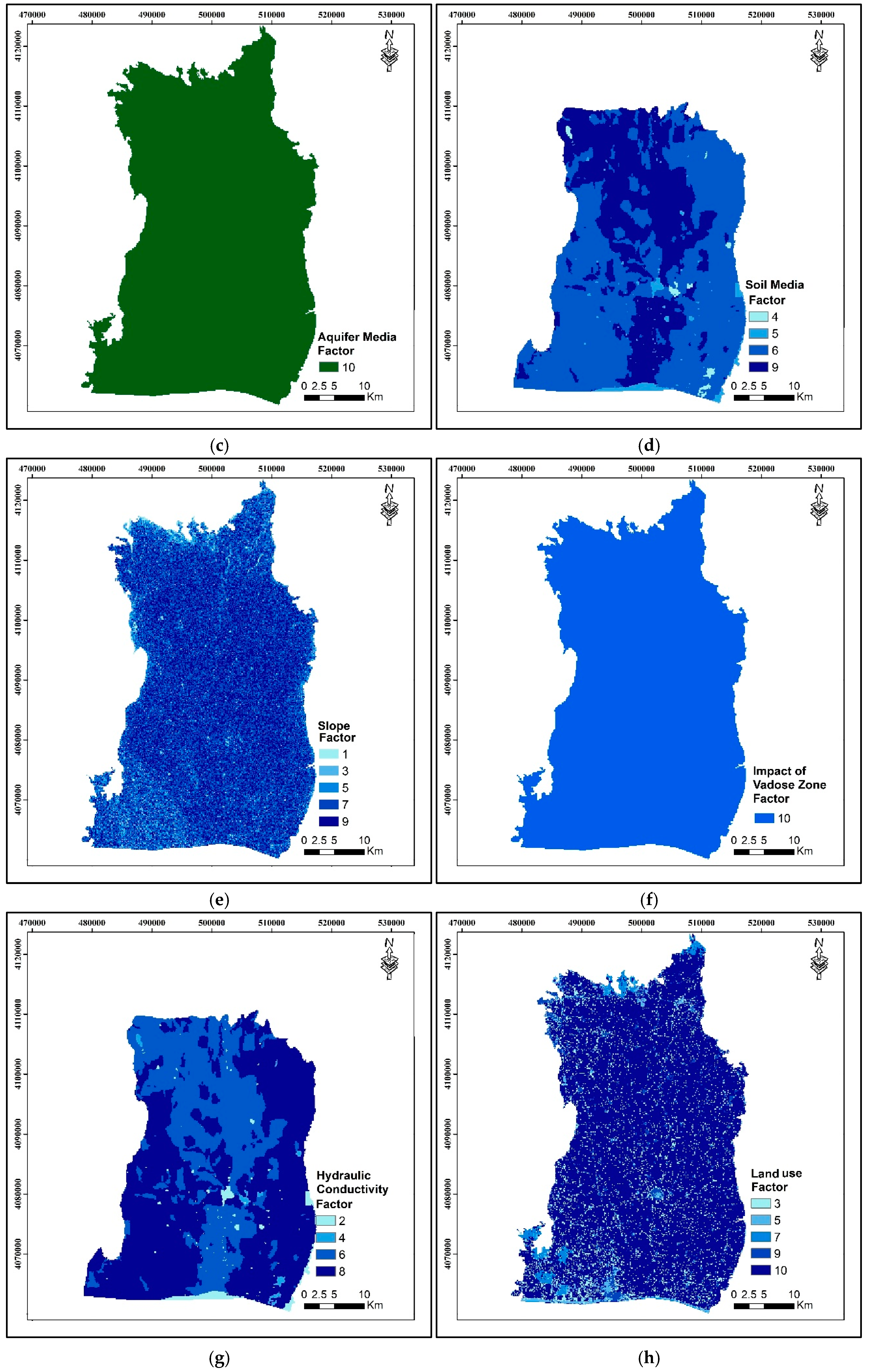
Both aquifer environment and vadose zone effect parameters of the Harran Plain were included in the DRASTIC vulnerability index model in accordance with the original framework proposed by Aller et al. [32]. Each parameter was assigned a weight value of 10, reflecting its critical role in groundwater vulnerability assessment. The geological structure of the plain is characterized by lithological homogeneity, particularly in terms of its aquifer and vadose zone properties. The plain is predominantly composed of karstified and fractured limestone formations, which exhibit similar permeability and porosity characteristics across the study area. Due to this spatial uniformity, the thematic layers representing these two parameters display limited visual variation in the resulting maps. However, their inclusion in the DRASTIC computation remains essential, as they capture the inherent hydrogeological attributes that influence contaminant transport and groundwater susceptibility.

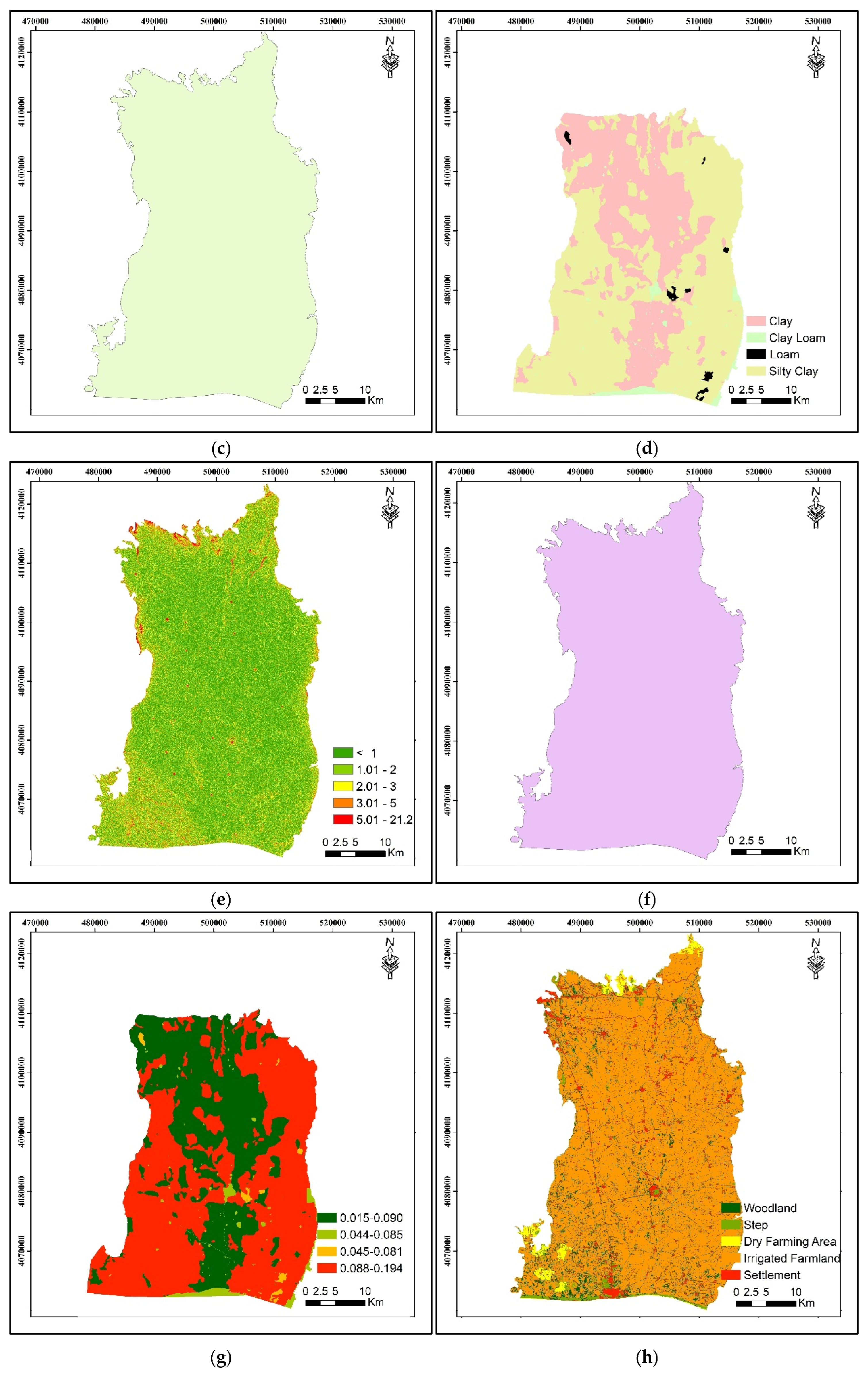
When the soil media of the Harran Plain is evaluated, alluvial, colluvial, and lacustrine are its primary constituents, generally containing clay and being slightly alkaline. The soils of the plain are classified as Vertisols, Inceptisols, and Entisols orders according to Soil Taxonomy [48]. The organic matter content of the soil is around 1% [49]. The very calcareous profile contains secondary lime accumulation with increasing density with depth. Profiles have A, B, and C horizons and have high cation exchange capacities. While organic matter decreases from the surface downwards, cation exchange capacities increase towards the lower layers depending on clay content [46,50,51]. The Harran Plain soils have a high lime content, with surface soils averaging 24% and deeper soils averaging 26%. The soil is rich in lime and poor in organic matter. The lowland soil contains 2:1 type clay with high swelling shrinkage, usually containing around 50% clay. The salt content of the soil is between ECe 1.0–37.9 (dS m⁻¹). While salinity cations are generally calcium, sodium is found in some parts of the plain [36,52]. Groundwater level (m) spatial distribution maps were produced using the interpolation method. The basin has a maximum water level depth of 20.80 m and a minimum of 1.03 m. Hydrogeological factors and thematic maps for ODM and MDM analyses are shown in Figure 4. To be used as a base map, satellite and DEM data with 30-m intervals were provided from the USGS [53] for the region’s topographic slope and land use. Criteria used for the DRASTIC framework are given in Figure 4.

2.3.2. Electrical Conductivity Data

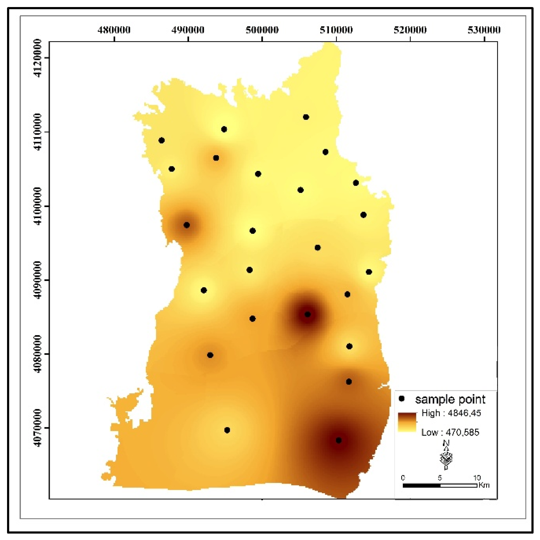
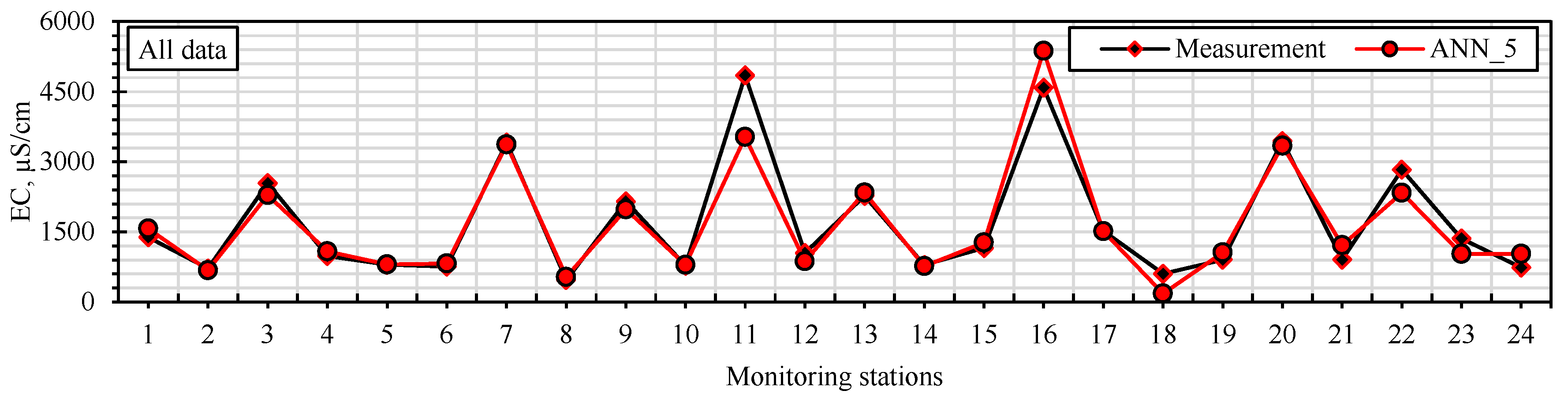
The spatial distribution map for the average values of EC measured at the groundwater sampling points in the study area is given in Figure 5.

EC values measured in the study area show significant differences according to the regions. Ugurlu (W11), Yardimli (W15), Ugrakli (W20), and Altılı (W24) have the highest EC values throughout the year. On the other hand, EC values were relatively low in areas such as Çekçek (W22), Yardımcı (W5), and Ikiagiz (W3). The areas with high EC values: Ugurlu (W11): the maximum EC value was 6870 µS/cm (October), and the average value was 3442 µS/cm. These values indicate that this region has significantly high EC levels. Yardimli (W15): the highest maximum EC value during the year was 8235 µS/cm (November), while the average value was 4848 µS/cm. This reveals that EC values in this region are both high and variable. Ugrakli (W20): the maximum EC value was recorded as 7068 µS/cm (October) with a mean value of 2828 µS/cm. A remarkable variability was observed with a standard deviation of 1629 µS/cm. The areas with low EC values: Çekçek (W22): the maximum EC value was 746 µS/cm (November), and the average was 469 µS/cm. This site has the lowest EC values. Yardimci (W5): the maximum EC value is 946 µS/cm (November), and the average is 604 µS/cm. Ikiagiz (W3): the maximum EC value is 1193 µS/cm (October), and the average is 738 µS/cm. Seasonal variations: the high EC values are generally monitored in October and November. Especially in the Ugurlu (W11), Yardimli (W15), and Altili (W24) regions, an increase was observed during these periods. Low EC values were generally recorded between May and August. This may be due to the decrease in salinity in the water with the effect of precipitation.

Elevated EC values observed at Ugurlu (W11) and Yardimli (W15) wells are spatially associated with low-lying zones of the southern Harran Plain, where intensive surface irrigation is practiced and drainage infrastructure remains insufficient. These areas are not adjacent to river channels or industrial sites but rather coincide with zones of irrigation return flow accumulation and shallow water table conditions. Additionally, the aquifer in these regions comprises relatively fine-grained alluvial sediments with lower permeability, impeding downward percolation and enhancing salt retention in the unsaturated zone. The spatial location of these wells aligns with the general direction of groundwater flow, reinforcing the interpretation that these are discharge zones where salinization is intensified. These findings suggest that both anthropogenic factors and hydrogeological characteristics jointly contribute to the observed salinity anomalies.

2.3.3. Target Data

The vulnerability index serves as the target data for predictive analytics and soft computing modeling groundwater contamination vulnerability assessments. Nevertheless, the vulnerability index derived from the ODM relies on subjective weights assigned to DRASTIC factors, as proposed initially by Aller et al. [32]. This subjectivity reduces the reliability of the resulting Original DRASTIC vulnerability index because the factor weights are arbitrarily determined [3,4,12]. EC values, on the other hand, are recognized as reliable indicators of groundwater contamination, as they are based on actual field measurements. These EC data are objective and reflect real-world conditions. In this study, the average values of monthly measured EC were used instead of NO₃-N values. The resulting index is termed AVI, and the following equation defines it:

$${\mathrm{A}\mathrm{V}\mathrm{I}}_{\mathrm{i}}={\displaystyle \frac{{\mathrm{M}\mathrm{D}\mathrm{V}\mathrm{I}}_{\mathrm{a}\mathrm{v}\mathrm{e}}}{{(\mathrm{E}\mathrm{C}-\mathrm{N})}_{\mathrm{a}\mathrm{v}\mathrm{e}}}}\times {(\mathrm{E}\mathrm{C}-\mathrm{N})}_{\mathrm{i}}\times {\displaystyle \frac{1}{\lambda }}$$

(2)

where MDVI_ave is the average value of all MDVI calculated by Equation (1); (EC − N)_ave is the average value of all measured EC data in the field; (EC − N)_i is an EC value at a sample location I; and λ is an arbitrary integer in 2 ≤ λ ≤ 6. The λ is necessary to make good AVI values close to MDVI values.

2.4. Predictive Analytics and Soft Computing Models

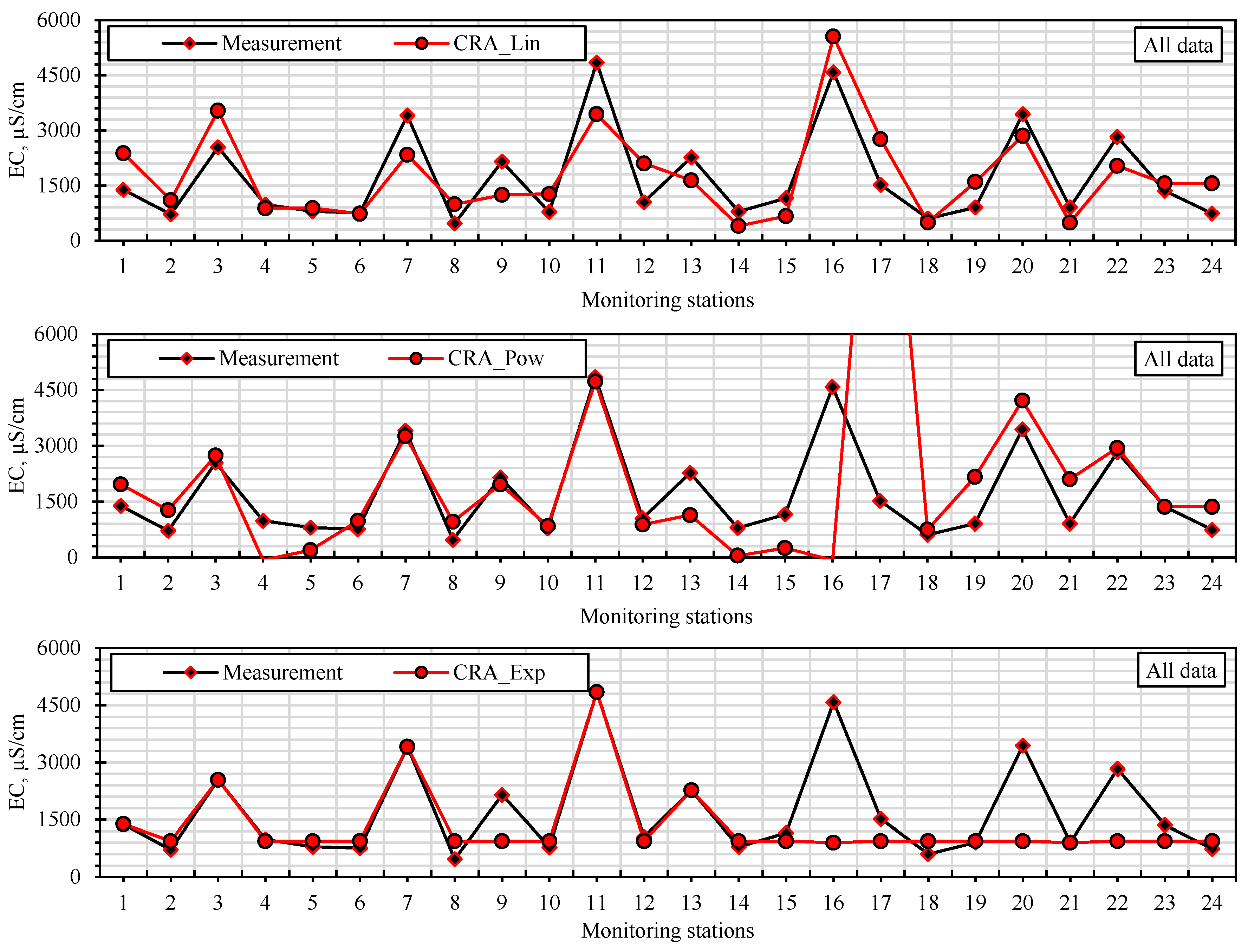
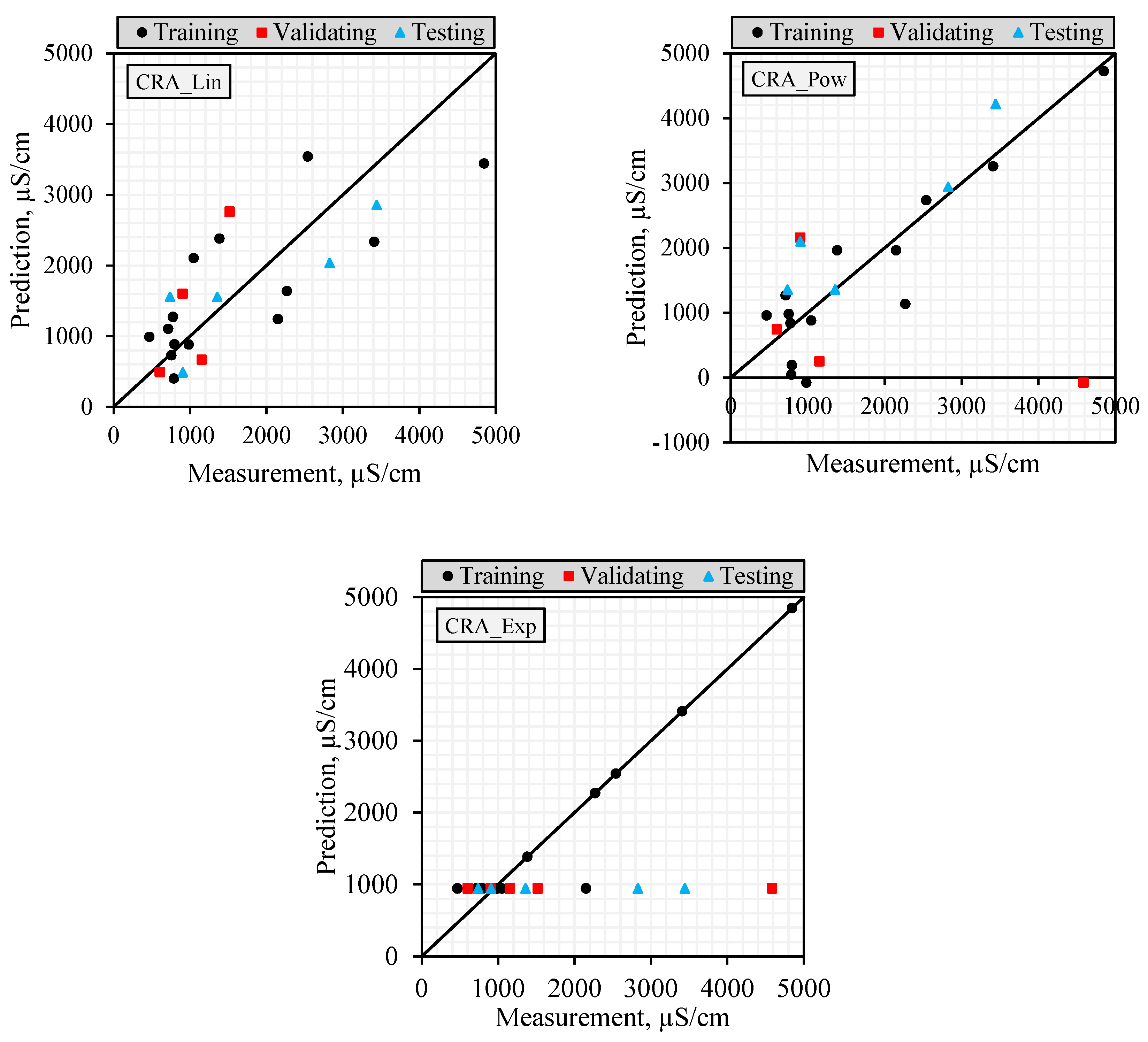
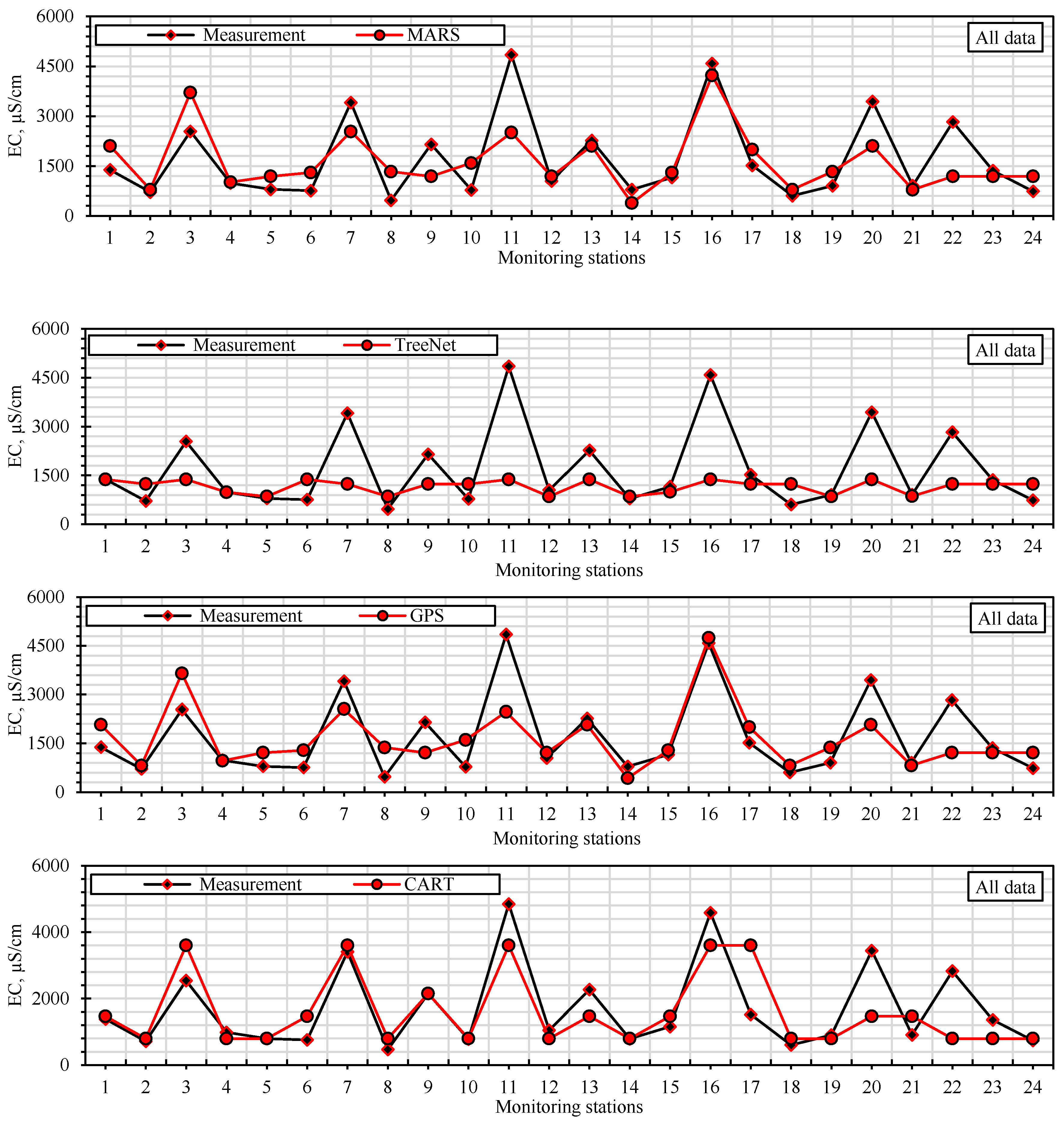
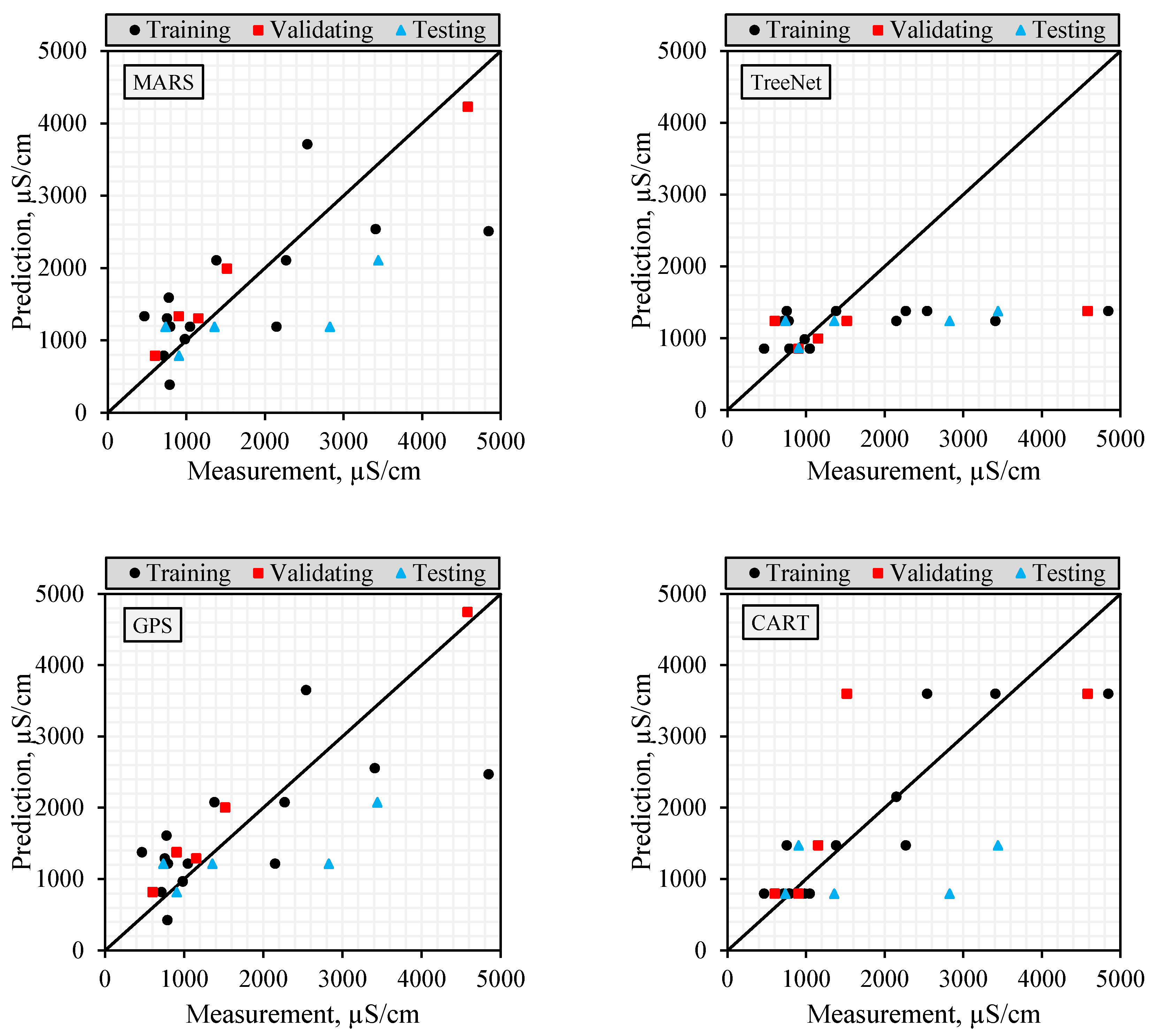
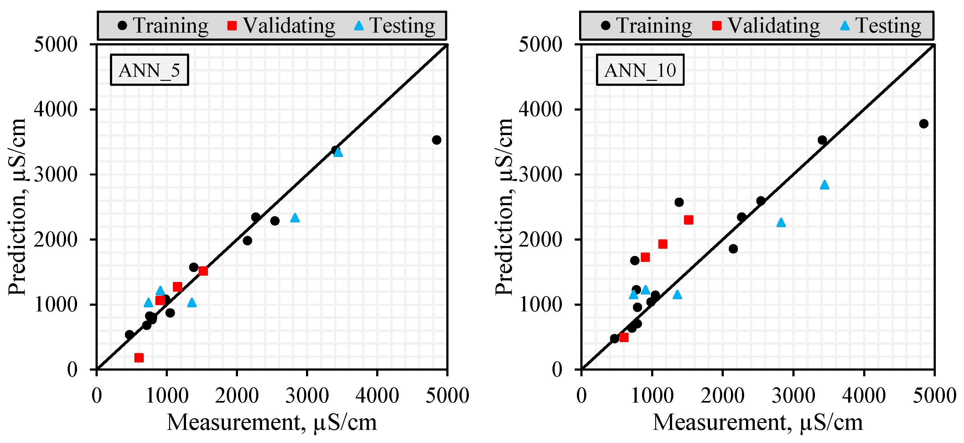
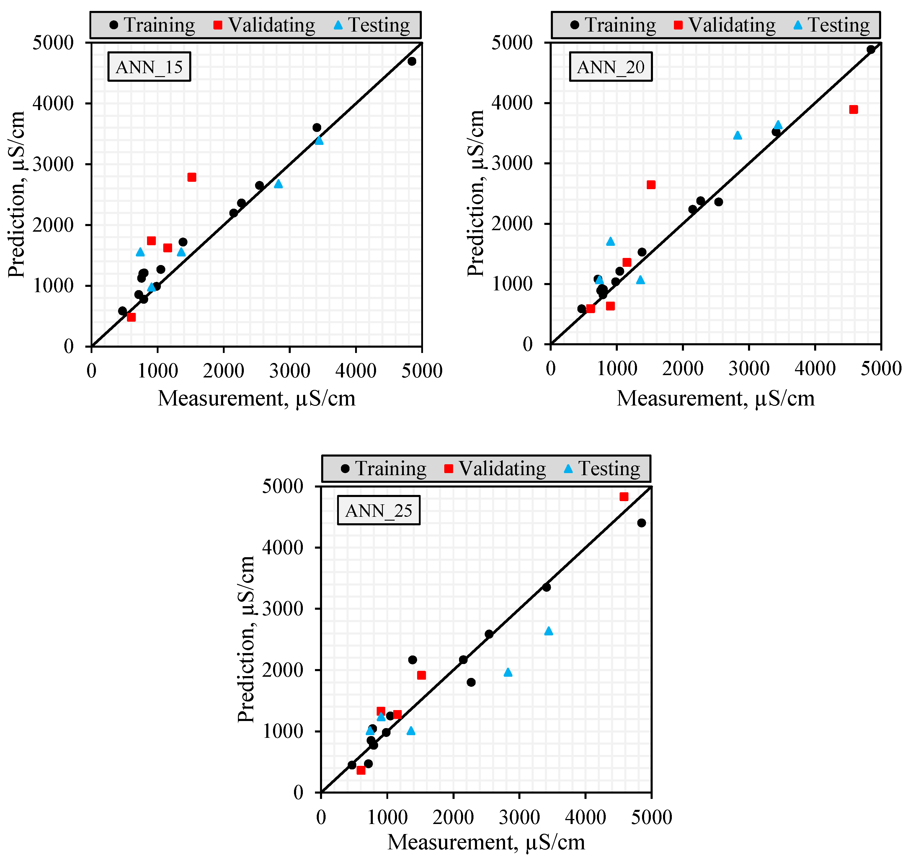
Predictive models were analyzed using regression-based models, soft computing models, and predictive analytics models. Soft computing models used: ANNs. The classical regression analysis was applied for three different equations (linear, power, and exponential). Predictive analytics models used: MARS [26], TreeNet [54], CART, and GPS.

ANNs are computational models based on biological neural networks and can learn relationships between independent and dependent variables. Once trained, they can predict experimental or observational data with high accuracy. Compared to traditional regression analysis, trained ANN models can produce reliable results with fewer computational requirements [55]. In addition, an essential advantage of the ANN method is that it can effectively model systems containing a large number of independent variables with minimal constraints [56,57].

The MARS is the first genuinely successful automated regression modeling tool in the world. Jerome Friedman is a world-renowned physicist and statistician from Stanford University. He developed MARS in the early 1990s. Explicitly designed to automate the construction of accurate prediction models for both continuous and binary dependent variables, MARS is an innovative and flexible modeling tool. One of the key strengths of MARS is its ability to easily find optimal variable transformations and potential interactions in any regression-based modeling solution while efficiently handling the complex data structure often hidden in high-dimensional data. As a result, this innovative technique in regression modeling effectively reveals crucial data patterns and relationships that are usually difficult, if not impossible, for other methods to identify [58].

TreeNet is a robust implementation of a class of modern machine learning algorithms commonly called stochastic gradient boosting. This technique is renowned for its superior predictive accuracy and was developed by Jerome Friedman at Stanford University [54]. The secret lies in how a model is built: each iteration adds a small tree to the existing ensemble of trees, correcting the ensemble’s combined errors. The process uses 3D plots to describe the nature of the dependence of the response variable on the model inputs and a variety of loss functions, including least squares regression, robust regression, and classification. The model is flexible enough for automatic detection and incorporation of various nonlinearities and multidirectional interactions [58].

CART is a tree-based algorithm that considers many different ways to partition, or divide locally, data into smaller segments based on other values and combinations of predictors. It selects the best-performing partitions and then iteratively repeats this process until an optimal set of partitions is found. The result is a decision tree represented by a set of binary splits leading to terminal nodes that can be defined by a set of specific rules [58]. CART is a method or an algorithm of the decision tree technique. CART is a non-parametric statistical method for describing the relationship between the response (dependent) quantity and one or more predictor quantities. Leo Breiman first proposed the CART method in 1984. The resulting CART decision tree is a binary tree. Each node must have two branches. CART is the recursive partitioning of the records in the training data into subsets that have the value of the target attribute (class) of the same. To select the most optimal branch for each node, the CART algorithm builds a decision tree. The selection is a count of all possibilities for each variable [59].

Traditional parametric models, such as linear and exponential regression, are based on assumptions including normal distribution of residuals, homoscedasticity, and linearity between variables. In groundwater pollution modeling, such assumptions are often violated due to the inherently nonlinear and heterogeneous nature of hydrogeological processes. Non-parametric models like ANNs and CART offer significant advantages in this context, as they do not impose strict assumptions on data distribution and are capable of capturing complex nonlinear relationships. This methodological flexibility contributes to higher predictive accuracy, particularly in datasets where multicollinearity, outliers, or non-constant variance are present.

The GPS is a flexible and advanced regression technique developed by Friedman [60] to overcome the modeling difficulties of traditional regression methods. It offers significant advantages, especially in cases where the number of independent variables exceeds the number of observations, there is a high correlation between variables, or more concise models are required. However, the GPS method is based on a linear and additive modeling approach; it can capture nonlinear relationships when the independent variables are appropriately determined. In addition, since it cannot directly handle missing data, it is necessary to eliminate data deficiencies before analysis [57].

2.5. Comparison of Model Prediction Performances

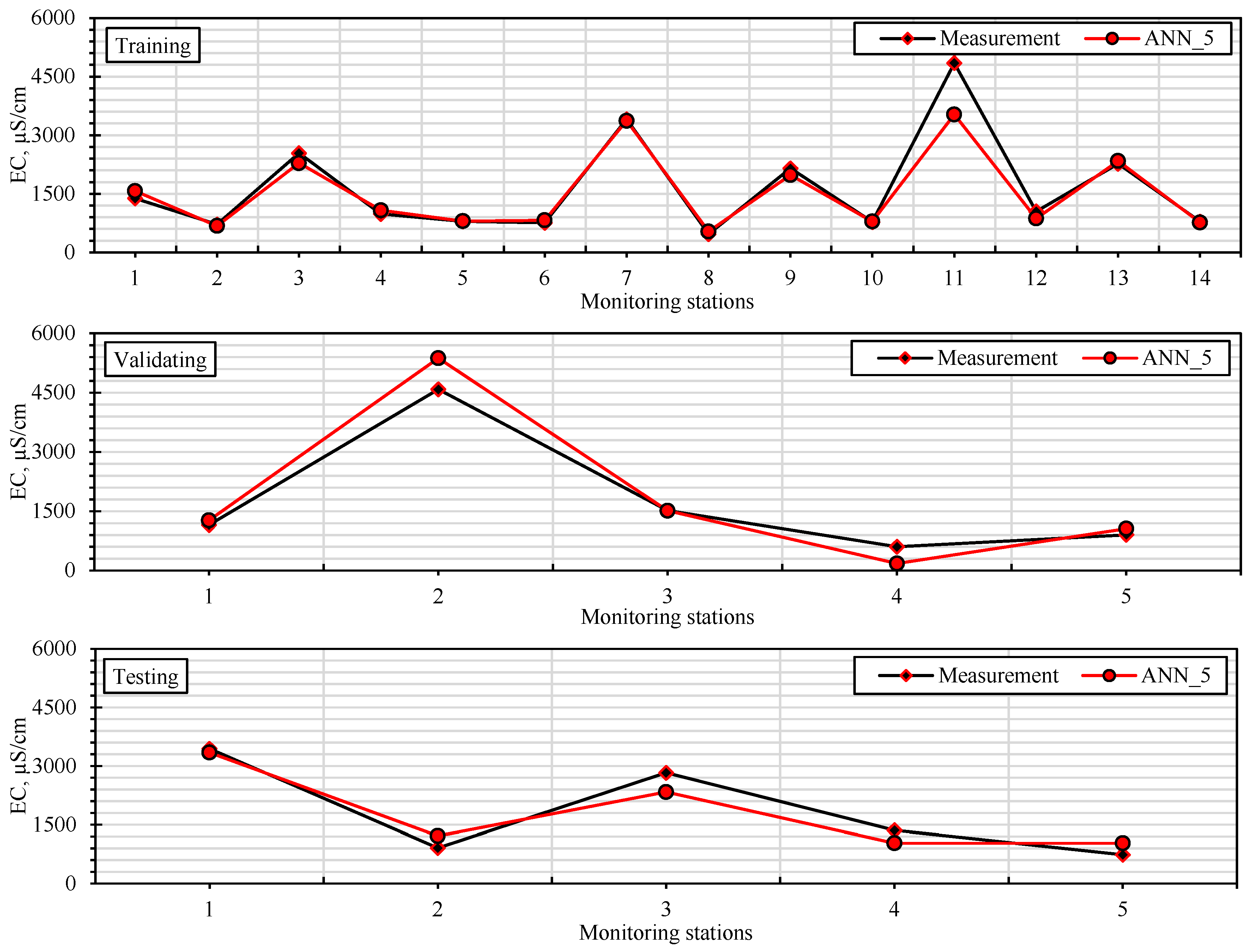
The datasets were divided into training, validating, and testing datasets to test the accuracy of the models established in the modeling studies. In this way, the accuracy of the models established with training and validating datasets could be evaluated using the testing dataset. The performances of the models were calculated using RMSE, MAE, and NS statistics given below.

$$\mathrm{RMSE}=\sqrt{{\displaystyle \frac{1}{\mathrm{N}}}{\sum }_{\mathrm{i}=1}^{\mathrm{N}}\left|{\left({\mathrm{t}}_{\mathrm{i}}-{\mathrm{t}\mathrm{d}}_{\mathrm{i}}\right)}^2\right|}$$

(3)

$$\mathrm{MAE}={\displaystyle \frac{1}{\mathrm{N}}}{\sum }_{\mathrm{i}=1}^{\mathrm{N}}\left|\left({\mathrm{t}}_{\mathrm{i}}-{\mathrm{t}\mathrm{d}}_{\mathrm{i}}\right)\right|$$

(4)

$$\mathrm{NS}=1-{\displaystyle \frac{{\sum }_{\mathrm{i}=1}^{\mathrm{N}}{\left({\mathrm{t}}_{\mathrm{i}}-{\mathrm{t}\mathrm{d}}_{\mathrm{i}}\right)}^2}{\sum _{\mathrm{i}=1}^{\mathrm{N}}{\left({\mathrm{t}}_{\mathrm{i}}-\overline{\mathrm{t}}\right)}^2}}$$

(5)

where t_i indicates measurement values; td_i indicates prediction values; $\overline{t}$ indicates the mean of measurement values; and n indicates the amount of data. While the performance of the method with smaller RMSE and MAE values is considered high, the NS value is between −∞ and 1. NS = 1 indicates that the technique used is perfect.

It is important to use more than one success criterion (NS, R², RMSE, and MAE) when evaluating model performance in order to reveal different aspects of the model’s error structure. While RMSE is sensitive to large errors and is more affected by extreme values, MAE reflects overall deviation more evenly as it evaluates all errors equally. R² indicates the similarity of the trend between the observed and predicted values, while NS is a normalized efficiency indicator that considers both variance and error magnitude. In this study, model reliability is assessed not only on the basis of a single metric but also through the combined interpretation of these four metrics, which are sensitive to different types of error. This multi-criteria approach provides a more accurate overall picture of forecasting success without exaggerating the impact of outliers on the model.

3. Results and Discussion

By using ArcGIS ArcMap 10.8, DRASTIC spatial distribution maps, which are ODM and MDM, were created for the unconfined aquifer of the Harran Plain that forms the study area.

Table 3. Assigned ratings of hydrogeological factors for thematic maps.

No.	Hydrogeological Factor	DRASTIC Range	Rating Value Based on DRASTIC Framework
1	Depth to water table (m)	(1.03–7.66), (7.67–12), (12.1–17), (17.1–20), (20.1–21.6)	(9), (7), (5), (3), (1)
2	Net recharge	(11.1–13), (9.1–11), (7.1–9), (5.1–7), (3–5)	(10), (8), (5), (3), (1)
3	Aquifer media	(Clay, Sand, and Gravel)	(10)
4	Soil media	(Clay), (Silty Clay), (Clay Loam), (Loam)	(9), (6), (5), (4)
5	Topographic slope (%)	(<1), (1–2), (2–3), (3–5), (>5)	(9), (7), (5), (3)
6	Impact of the vadose zone	(Clay, Sand, and Gravel)	(10)
7	Hydraulic conductivity (m/d)	(0.042–0.081), (0.045–0.081), (0.015–0.090), (0.088–0.194)	(2), (4), (6), (8)
8	Land use	(Irrigated Farmland), (Settlement), (Dry Farming Area), (Step), (Woodland)	(10), (9), (7), (5), (3)

provides assigned ratings of hydrogeological factors for thematic maps shown in Figure 6.

In this case, when the ODM and MDM maps are compared, it is seen that nearly half of the plain, especially in the areas close to the urban settlements, is susceptible to pollutants. In addition, due to the rise of surface waters, potential contaminants for the plain pose a risk for groundwater. The ODM and MDM thematic maps are shown in Figure 7. The results show that the modified model considers more factors and provides a more sensitive analysis than the original model. In the MDM, the addition of land use as an essential factor has led to the identification of areas with higher sensitivity, especially in agricultural and residential areas. Figure 7 shows that the MDM predicts the pollution potential more effectively, especially in areas close to residential areas.

3.1. Performance of Predictive Analytics and Soft Computing Models

3.1.1. CRA Results

Table 4. Results of classical regression analysis.

Dataset	Performance Statistics	CRA_Lin	CRA_Pow	CRA_Exp
Training	RMSE (µS/cm)	769	561	364
	MAE (µS/cm)	649	448	193
	NS	0.60	0.79	0.91
Validating	RMSE (µS/cm)	803	6351	1658
	MAE (µS/cm)	702	4056	961
	NS	0.69	−18.27	−0.31
Testing	RMSE (µS/cm)	610	695	1415
	MAE (µS/cm)	563	540	1008
	NS	0.68	0.59	−0.71

presents the performance statistics obtained by applying the CRA method to the three functions. According to Table 4, the CRA Pow and CRA Exp models gave high-performance values for the training dataset, but the same was not the case for the validating and testing datasets. The CRA Exp model, which gave the highest performance value for the training dataset, gave an NS value of −0.71 for the testing dataset. These results indicate that using the average values for the testing dataset will perform better than the prediction values. The same was true for the CRA Pow model. The findings indicate that the CRA Pow and CRA Exp models are not sufficient in predicting EC data and are unsuitable to be used. In addition, the CRA Lin model yielded reasonable results for all three datasets. The NS values of the CRA Lin model are 0.60, 0.69, and 0.68 for training, validating, and testing datasets, respectively. In light of these findings, it can be stated that the CRA Lin model shows sufficient performance values in predicting EC data. It can be recommended as a usable model for groundwater quality prediction studies.

To compare the prediction performances of the models, the time series of all datasets, where training, validating, and testing datasets are all together, and the scatter diagrams, where each dataset is colored separately, are given in Figure 8. When the time series are analyzed, it is seen that the CRA Lin model gives prediction values close to the measurement values for all monitoring stations. On the other hand, the rest two models either underestimate or overestimate the values for some stations. In the scatter diagrams, it is especially clear that the CRA Exp model produces a single value for the validating and testing datasets. It is observed that the CRA Pow model predicts some values as lower than 0, which is impossible in reality.

3.1.2. Predictive Analytics Models Results

The performance statistics of the models developed using MARS, TreeNet, GPS, and CART methods are given in

Table 5. Predictive analytics model results.

Dataset	Performance Statistics	MARS	TreeNet	GPS	CART
Training	RMSE (µS/cm)	891	1219	892	540
	MAE (µS/cm)	678	780	678	355
	NS	0.47	0.01	0.47	0.80
Validating	RMSE (µS/cm)	343	1468	329	1044
	MAE (µS/cm)	317	866	292	736
	NS	0.94	−0.03	0.95	0.48
Testing	RMSE (µS/cm)	972	1187	973	1315
	MAE (µS/cm)	743	863	738	1037
	NS	0.19	−0.20	0.19	−0.48

for training, validating, and testing datasets.

It can be seen that the highest performance value for the training dataset was obtained from the CART method. Although the CART method was followed by the MARS and GPS methods for the training dataset, the performance values obtained from these methods were not considered acceptable. The worst performance values were obtained from the TreeNet method. On the other hand, the highest performance values for the validating dataset were obtained from the GPS method. It was followed by MARS and CART methods, respectively. When it comes to the testing dataset, it was concluded that the performance values of the four methods were low and these methods could not be used.

The time series comparisons of the measurement data and the prediction values obtained for the four methods are given in Figure 9. In addition, scatter diagrams of the prediction methods and models are also provided using different symbols for each of the three datasets.

When the time series are analyzed, it is seen that although MARS, GPS, and CART methods produced the prediction values close to the actual values for some stations, they could not predict many station values, especially for the validating and testing datasets. This is also clearly visible in the scatter diagrams. In addition, it is seen that the TreeNet method is not able to predict the actual values successfully and produces a fixed value as a prediction value in almost more than half of the stations. In the CART method, similar results are possible for three different constant values.

3.1.3. ANNs Model Results

The performance statistics of the highest-performing models from the models developed using five different neuron numbers (5, 10, 15, 20, and 25) in the ANNs method are given in

Table 6. Artificial neural networks model results for different number of hidden layer neurons.

Dataset	Model	ANN_5	ANN_10	ANN_15	ANN_20	ANN_25
Training	RMSE (µS/cm)	371	518	235	150	295
	MAE (µS/cm)	181	331	188	128	192
	NS	0.91	0.82	0.96	0.98	0.94
Validating	RMSE (µS/cm)	410	662	889	609	306
	MAE (µS/cm)	299	606	776	460	286
	NS	0.92	0.79	0.62	0.82	0.96
Testing	RMSE (µS/cm)	329	446	386	506	581
	MAE (µS/cm)	304	420	258	451	522
	NS	0.91	0.83	0.87	0.78	0.71

.

It is seen from Table 6 that the highest performance values for the training dataset are obtained from the model with 20 neurons. RMSE, MAE, and NS values are calculated as 150 µS/cm, 128 µS/cm, and 0.98, respectively. This model is followed by the models with 15, 25, 5, and 10 neurons, respectively. When it comes to the performance values calculated for the validating dataset, it is determined that the model with the highest performance is the model with 25 neurons. The closest performance values to this model are obtained from the ANN_5 model. When the performance statistics calculated for the testing dataset are examined, it is seen that the highest performance values are obtained from the ANN_5 model. As can be seen from Table 6, the models with different neurons produced the highest performance values in all three datasets. In this case, when Table 6 is evaluated in general for all three datasets, the ANN_5 model is assessed as the highest-performing model in all three datasets. The NS values obtained from the ANN_5 model are 0.91, 0.92, and 0.91 for the training, validating, and testing datasets, respectively, and it can be stated that these values are in the very high-performance model class for the NS criterion. When Table 6 is analyzed, it is possible to say that using a different number of neurons in the ANNs method has significant effects on model performances. However, it is not possible to say that the increase in the number of neurons affects the model performance. In other words, the rise in the number of neurons in ANN-based models developed for the prediction of EC values did not increase the model performance.

The scatter diagrams of the models are given in Figure 10. It is seen from Figure 10 that the values of the ANN_5 model are distributed on the diagonal, while the predicted values of the other models are farther away from the diagonal compared to the ANN_5 model.

The measurement values and the prediction values of the ANN_5 model, which gives the highest performance values among the ANN models, are shown in Figure 11 as time series for the entire dataset and the training, validating, and testing datasets, respectively. When the time series are examined, it is seen that the predicted values for all three datasets produce values very close to the real values. It is possible to say that the prediction values and the measurement data, especially for the training dataset, overlap, and there are very small differences between them. In addition, it is clearly seen that the five station values in the validating and testing datasets are very close to the real values.

To assess whether the difference between the observed and predicted values in the training dataset is statistically significant, a paired-sample t-test was performed. In this test, the null hypothesis (H₀) is based on the assumption that there is no significant difference in the mean between the two datasets. The results of the test show that the p-values for all models are above the 0.05 significance level. This indicates that there is no statistically significant difference between the observed and predicted values, which confirms the graphical observation of ‘near overlap’ statistically.

The results presented in

Table 7. Pearson’s correlation coefficients (R) between models and EC values.

* Models	R	* Models	R
ODM	−0.4556	MARS	0.4796
MDM	−0.4556	TreeNet	0.4679
ANN_5	0.5591	GPS	0.5027
ANN_10	0.4962	CART	0.3674
ANN_15	0.4937	CRA_Lin	0.4645
ANN_20	0.4555	CRA_Pow	0.0359
ANN_25	0.4588	CRA_Exp	0.4801

Note: * Using training and testing datasets (overall performance).

evaluate the accuracy of different models in predicting EC data using R values.

The results in Table 7 allow a comparative evaluation of the linear relationships of the models with EC values and their predictive performance accordingly. Among the ANN models, the ANN_5 model showed the best performance with an R-value of 0.5591. It is followed by the models ANN_10 (0.4962), ANN_15 (0.4937), ANN_25 (0.4588), and ANN_20 (0.4555), respectively. This indicates that increasing the number of layers or parameters of the ANNs models does not always have a positive effect on the prediction performance.

The ODM and MDM indicate a weak relationship with an R-value of −0.4556. This result shows that these models are not suitable for the EC prediction and show an opposite prediction trend. On the other hand, the MARS (0.4796), TreeNet (0.4679), and GPS (0.5027) models are partially successful in predicting EC data with moderate positive R values. The GPS model has the highest R value among these three models and provides relatively better prediction accuracy. While the CART model lags behind the other models with an R-value of 0.3674, the CRA Lin (0.4645), CRA Exp (0.4801), and CRA Pow (0.0359) models showed different levels of performance. The fact that the R-value of the CRA Pow model is relatively low (0.0359) shows that this model has a weak linear relationship in the prediction of EC values. Therefore, its prediction performance is somewhat limited. When these results are evaluated in general, the ANN_5 and GPS models stand out as successful prediction tools. However, the low performance of the ODM and MDM models indicates that it is not appropriate to consider these models in the prediction processes. In conclusion, this analysis provides an essential guide for determining which models offer higher accuracy in predicting EC data and for model selection in future studies. Spatial distribution maps of predictive analytics and soft computing models for groundwater contamination vulnerability are shown in Figure 12.

4. Conclusions

This study employed an integrated hydrogeochemical and multivariate statistical approach to unravel the complex interplay of natural and anthropogenic factors influencing groundwater quality in the Harran Plain, a vital agricultural hub within Türkiye’s GAP region. Key findings revealed that groundwater composition is predominantly controlled by evaporate mineral dissolution (e.g., gypsum and halite) and anthropogenic inputs from intensive agriculture and inadequate wastewater systems. While most groundwater samples met permissible limits for domestic and agricultural use, localized zones exhibited critical elevations in nitrate, chloride, and sulfate concentrations, highlighting spatial heterogeneity in contamination risks. These results align with global observations of groundwater vulnerability in semi-arid, irrigation-intensive regions, but they also advance the field by demonstrating that we can distinguish between overlapping geochemical and human-driven processes in complex settings.

This study’s methodological framework, combining traditional hydrochemistry with robust statistical analysis, provides a replicable model for assessing groundwater quality in similar agro-industrial basins. However, its spatial restriction to a single basin and reliance on a single sampling campaign limit insights into seasonal variations and long-term trends. Furthermore, while statistical clustering clarified dominant processes, isotopic or trace element analyses could enhance source apportionment of contaminants like nitrate.

Future research should prioritize longitudinal monitoring to capture temporal dynamics and expand geographically to assess groundwater responses across diverse hydrogeological and land-use zones within the GAP region. Integrating machine learning with remote sensing and GIS data could further improve predictive capacity for contamination hotspots. Practically, the findings advocate for the following immediate actions: (i) targeted monitoring of high-risk zones identified in this study; (ii) stricter enforcement of sustainable agricultural practices (e.g., optimized fertilizer use and wastewater treatment); and (iii) investment in drainage infrastructure to mitigate salinity build-up.

Ultimately, by bridging empirical hydrogeochemical insights with practical groundwater-management strategies, this study provides policymakers and water authorities with evidence-based tools to strengthen groundwater sustainability and secure water resources in agriculturally critical, water-scarce regions. Preliminary piezometric mapping suggests an increased hydraulic gradient that may support two-dimensional (lateral and vertical) groundwater flow, particularly near the alluvial-bedrock interface and in zones of elevation change. However, as the DRASTIC-based vulnerability model was primarily designed for assessing vertical susceptibility of groundwater to surface contamination, the lateral flow dynamics were not explicitly integrated into the index calculations. We acknowledge this as a limitation of the current framework to clarify that two-dimensional flow conditions, especially in areas of steep hydraulic gradients, may influence contaminant migration pathways in ways not fully captured by the model. To improve future vulnerability assessments, we suggest that modified index approaches or physically based numerical models (e.g., MODFLOW-based simulations) be used in combination with DRASTIC to incorporate lateral flow and anisotropic hydraulic conditions more accurately. Although the aquifer media and vadose zone layers exhibited limited spatial variability across the study area, primarily due to the resolution of national-scale geological data and borehole logs, they were retained in the analysis for methodological consistency with the standard DRASTIC model framework. These parameters conceptually represent subsurface properties such as vertical permeability and contaminant attenuation capacity, which are critical for understanding intrinsic vulnerability. Future studies may benefit from the incorporation of higher-resolution subsurface data to improve the spatial representativeness and analytical robustness of these layers.