Abstract
Estuarine ecosystems, characterized by dynamic salinity gradients and complex physicochemical interactions, serve as critical transition zones between freshwater and marine environments. This study investigates the spatial evolution of sediment microbial communities across a freshwater–seawater continuum and their correlations with water quality parameters. Five sampling zones (upstream, midstream, downstream, transition zone, and ocean) were established in a typical estuary (Kuiyu Park, China). High-throughput 16S rRNA sequencing revealed significant shifts in microbial composition, with dominant phyla including Firmicutes, Bacteroidetes, Proteobacteria, and Actinobacteria. Alpha diversity decreased from freshwater to the transition zone but rebounded in seawater, suggesting habitat filtering and niche differentiation. Redundancy analysis identified salinity, dissolved oxygen, nutrients, and heavy metals as key drivers of microbial community structure. Functional predictions highlighted metabolic adaptations such as methanogenesis, sulfur oxidation, and aerobic chemoheterotrophy across zones. This study explores how sediment microorganisms adapt to water quality variations during the freshwater–seawater transition, offering insights into estuarine resilience under global change. These findings elucidate microbial assembly rules in estuarine ecosystems and provide insights for ecological management under global environmental change.
1. Introduction
The estuarine ecosystem encompasses the interaction between various types of organisms in the estuarine water body and their relationship with the estuarine environment. It is a transitional ecosystem at the confluence of rivers and the sea, with both freshwater and seawater characteristics, and is one of the most productive and biologically diverse natural environmental systems on earth [1]. The system is affected by multiple factors, including natural factors, tidal action, changes in salinity gradients, climate change, chemical factors, production and domestic sewage, and global warming due to the greenhouse effect [2]. When freshwater and seawater mix with each other, the difference in salinity leads to the formation of salinity stratification, while the difference in density drives the gravity circulation, where freshwater flows to the surface layer of the sea, seawater invades to the bottom layer of the land, forming the typical circulation pattern in estuaries [3], and the suspended particles carried by freshwater, such as sediment and organic matter. Flocculation and sedimentation will occur in the case of seawater electrolytes, which will lead to a change in turbidity and the phenomenon of metal sedimentation, triggering a series of complex physical, chemical, and biological changes [4]. These changes can significantly affect estuarine microorganisms. These changes will also significantly affect the community structure, function and ecological processes of estuarine microorganisms [5]. The change in salinity gradient will lead to an increase in a large number of salt-adaptable microorganisms in estuaries, and the hypoxia at the bottom will also result in a reduction in aerobic bacteria and the proliferation of anaerobic sulfate-reducing bacteria [6]. The nitrogen or phosphorus input from fresh water increases organic matter and promotes the proliferation of heterotrophic bacteria [7].
In the estuarine ecological environment, during the transition from freshwater to seawater, the microorganisms in the sediments have a close relationship with water quality indicators [8]. Salinity is a key water quality indicator in the ecological environment of estuaries and has an important influence on the structure and function of sediment microbial communities [9]. As the transition from fresh water to seawater increases, the salinity gradually rises, and different microorganisms have different adaptability levels to salinity. Salt-tolerant microorganisms can adapt to salinity changes by regulating intracellular osmotic pressure and synthesizing compatible solutes, and gradually gain an advantage in high-salinity environments [10]. Therefore, changes in salinity will screen out different microbial communities, causing alterations in the structure of microbial communities in sediments. The dissolved oxygen content determines whether the living environment of microorganisms is aerobic or anaerobic [11]. In anoxic or anaerobic zones, anaerobic microorganisms such as methanogens and sulfate-reducing bacteria play a major role, carrying out metabolism through processes such as fermentation and sulfate reduction [12]. The variation in dissolved oxygen content in water bodies will affect the types and quantity distribution of microorganisms. For instance, in areas with a higher dissolved oxygen content, there are more aerobic microorganisms, while in areas with a lower dissolved oxygen content, anaerobic microorganisms are more abundant. Nutrients are the material basis for the growth and reproduction of microorganisms [13]. Different types of microorganisms have different demands and utilization capabilities for nutrients, so the composition and proportion of nutrients also affect the structure of microbial communities. Heavy metals have toxic effects on microorganisms and can inhibit their growth, metabolism and reproduction [14]. High concentrations of heavy metal ions may combine with biological macromolecules such as enzymes and proteins within microbial cells, causing their activity to be lost and thereby affecting the normal physiological functions of microorganisms [15]. When exposed to an environment containing heavy metals for a long time, the microbial community will undergo adaptive changes. Some microorganisms with heavy metal resistance genes gradually become dominant populations.
In this study, we take a typical estuarine ecosystem as the research object. This area is a convergence zone of freshwater and seawater, characterized by a compact spatial scale from freshwater zones to transition zones and then to marine areas, making it convenient for sampling while exhibiting a pronounced salinity gradient. We divided the system into five research areas (from freshwater to seawater), namely the upstream (US), midstream (MS), downstream (DS), transition zone (TZ), and ocean (OC). In these five areas, we collected sediment and water samples, respectively. The sediment was used for the analysis of the diversity of environmental microorganisms, and at the same time, multi-index analysis was carried out on the water body. Through the regional evolution laws of environmental microorganisms and the variation laws of water quality indicators, we explored their correlations. This study established a correlation between environmental microorganisms and water quality gradient changes in typical estuarine ecosystems, providing molecular ecological evidence for the resilience assessment of estuarine ecosystems under the background of global environmental changes [16]. It has deepened our understanding of the microbial ecological processes in the “land–sea continuum” and also provided a theoretical basis for the protection of biological resources and pollution control in estuarine areas [17].
2. Materials and Methods
2.1. Study Area and Sampling Design
This study selected a typical estuarine ecosystem (Kuiyu Park in Quanzhou, China) as the research object (Figure 1). This park has obvious characteristics of salinity gradient changes, providing an ideal place to explore the evolution law of microbial communities during the transition from freshwater to seawater [18]. Sampling work was carried out in November 2024 and this timeframe was selected because November in Quanzhou (subtropical monsoon climate, 24.9° N) typically features mild air temperatures (15–25 °C) [19] and stable hydrological conditions after the summer monsoon season [20], minimizing flood disturbances and algal bloom impacts [21] while supporting active microbial metabolism [22]. These conditions facilitate clear spatial resolution of salinity-driven microbial patterns without confounding seasonal variability [23]. Based on the previous investigation and the analysis of hydrological characteristics, five representative sampling stations were set up along the salinity gradient [6]. US is located at the very upper reaches of the estuary. MS and DS are located in the middle and lower reaches of the estuary. TZ is located in the estuary area. OC is located in the outer sea area of the estuary. The sampling work of sediments strictly follows the principles of “random quantification” and “multi-point mixing” to reduce the influence brought by environmental heterogeneity and sampling errors [24]. At each sampling station, five sampling points were set up using the grid method, and sterile stainless steel samplers were used to collect surface sediments.
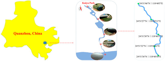
Figure 1.
Sampling sites in Kuiyu Park in Quanzhou, China.
The field parameters included water temperature (Tem), pH, dissolved oxygen (DO), electric conductivity (EC), salinity (Sal) and transparency (TR), which were directly measured using a multi-parameter water quality analyzer (YSI, Yellow Springs, OH, USA) [18]. Each parameter should be measured at least three times and the average value should be taken. The concentration of chlorophyll a (Chl-a) was determined on-site by the fluorescence method [25]. Laboratory data analysis was carried out immediately after the water samples were collected. The concentrations of total nitrogen (TN), ammonia nitrogen (NH4+-N), nitrate nitrogen (NO3−-N), nitrite nitrogen (NO2−-N) and total phosphorus (TP) were determined by a continuous flow analyzer (SEAL Analytical, Fareham, UK) [26], and the contents of heavy metals (Cu, Pb, Zn, Cd, Hg, Se) were analyzed by an inductively coupled plasma mass spectrometer (Thermo Fisher Scientific, Waltham, MA, USA) [27]. The particle size composition was determined by a laser particle size analyzer (Malvern Instruments, Worcestershire, UK) [28]. All chemical analyses were subject to quality control with blank controls and standard reference substances, with the relative standard deviation controlled within 5%.
2.2. DNA Extraction and PCR Amplification
Total genomic DNA was isolated from sediments utilizing a cetyltrimethylammonium bromide CTAB-based protocol [29]. DNA quality and concentration were evaluated via 1% agarose gel electrophoresis. Purified DNA was normalized to 1 ng/μL using sterile water. The hypervariable V3–V4 regions of bacterial 16S rRNA genes were amplified via PCR with barcoded primers 341F (5′-CCTAYGGGRBGCASCAG-3′) and 806R (5′-GGACTACNNGGGTATCTAAT-3′) [30]. Reaction mixtures contained 15 μL Phusion® High-Fidelity PCR Master Mix (New England Biolabs, Ipswich, MA, USA), 2 μM each of forward and reverse primers, and approximately 10 ng of template DNA. Thermocycling conditions included an initial denaturation at 98 °C for 1 min, followed by 30 cycles of denaturation (98 °C, 10 s), annealing (50 °C, 30 s), and extension (72 °C, 30 s), with a final elongation at 72 °C for 5 min [31]. Amplified products were electrophoresed on 2% agarose gels in 1×TAE buffer for verification. Equimolar PCR amplicons were pooled and purified using the Universal DNA Purification Kit (TIANGEN, Beijing, China).
2.3. Library Preparation and Illumina NovaSeq Sequencing
Sequencing libraries were constructed using the NEB Next® Ultra DNA Library Prep Kit (Illumina, San Diego, CA, USA) following the manufacturer’s protocol, with unique indices incorporated for sample differentiation [32]. Library quality was verified using an Agilent 5400 Bioanalyzer (Agilent Technologies, Santa Clara, CA, USA). Paired-end sequencing (250 bp reads) was performed on the Illumina NovaSeq platform [33].
2.4. Statistical Analysis
Data are presented as mean ± standard deviation (SD). Intergroup comparisons were analyzed using ANOVA. Statistical significance thresholds were set at * p < 0.05, ** p < 0.01, and *** p < 0.001. Based on the normalized OTU species abundance profiles, further analysis of OTU abundance and diversity indices was conducted, followed by statistical analysis of community structure across taxonomic levels based on species annotation. Analyses were conducted using GraphPad Prism 8 (GraphPad Software Inc.; San Diego, CA, USA) and the Wekemo Bioincloud platform (https://www.bioincloud.tech, accessed on 5 May 2025).
3. Results and Discussion
3.1. Spatial Differences of Microbial Communities
In this study, the 16S rRNA gene amplicon high-throughput sequencing technology combined with multidimensional bioinformatics analysis and obtained high-resolution amplicon sequence variants (ASVs) for visual analysis were used to systematically analyze the composition characteristics, spatial differences, functional metabolic potential of the sediment microbial community in the target area and its coupling mechanism with environmental factors [24]. To systematically analyze the changes in the percentage of microorganisms in different groups, this study presented the distribution of the top 20 species in terms of abundance in each group at six different levels: phylum, class, order, family, genus, and species. The microbial community composition at the phylum level across the five sample groups (US, MS, DS, TZ, OC) revealed distinct taxonomic patterns (Figure 2). At the phylum level, Firmicutes dominated freshwater zones (US: 38.2%, MS: 34.5%), likely due to their prevalence in anaerobic, sulfate-rich sediments (e.g., Desulfovibrio spp.) [12]. In contrast, Bacteroidetes increased in brackish zones (DS: 29.1%, TZ: 33.7%), correlating with elevated organic matter degradation [34]. Marine zones (OC) showed a marked shift toward Proteobacteria (26.8%), particularly Gammaproteobacteria, known for their halotolerance and metabolic versatility in saline environments [20]. At the class level within Firmicutes, the class Clostridia (US: 28.4%, MS: 25.1%) dominated freshwater sediments, suggesting active fermentation and sulfate reduction [12]. In marine zones, Gammaproteobacteria (OC: 21.3%) prevailed, aligning with their role in aerobic heterotrophy and sulfur cycling [35]. Brackish zones (TZ) exhibited a mix of Bacteroidia (18.9%) and Alphaproteobacteria (12.5%), indicating transitional metabolic strategies [36]. The order Desulfovibrionales (phylum Firmicutes) was enriched in US (15.2%) and MS (13.8%), supporting sulfate reduction under low-oxygen conditions [12]. In OC, Alteromonadales (order within Gammaproteobacteria) accounted for 9.7% of sequences, reflecting adaptations to high salinity and organic carbon availability [20]. Families such as Desulfovibrionaceae (US: 12.1%) and Rhodocyclaceae (TZ: 8.4%) highlighted niche-specific functions—sulfate reduction in freshwater and denitrification in brackish zones, respectively. The marine family Vibrionaceae (OC: 6.9%) was linked to polysaccharide degradation in algal-rich habitats. Key genera included Desulfovibrio (US: 10.5%), Thiobacillus (TZ: 7.2%), and Pseudomonas (OC: 5.8%). Desulfovibrio’s dominance in freshwater zones correlated with sulfate reduction [12], while Thiobacillus in TZ suggested sulfur oxidation under fluctuating redox conditions. Pseudomonas in OC indicated hydrocarbon degradation potential [37]. Species-level resolution revealed Desulfovibrio vulgaris (US: 4.3%) and Thiobacillus thioparus (TZ: 3.1%) as functional markers for sulfate reduction and sulfur metabolism, respectively. Marine zones harbored Pseudomonas aeruginosa (OC: 2.9%), a known hydrocarbon degrader, underscoring anthropogenic pollutant impacts [37].
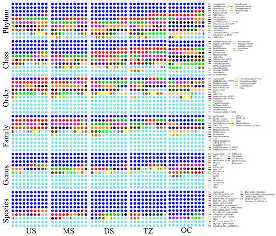
Figure 2.
Structural variations in microbial communities across taxonomic hierarchies (phylum to species).
Dominant phyla identified included Firmicutes, Bacteroidetes, Proteobacteria, and Actinobacteria, which collectively accounted for the majority of the microbiota in all groups [38]. Notably, Firmicutes exhibited the highest relative abundance in groups US and MS, whereas Bacteroidetes dominated in DS and TZ [20]. Group OC displayed a more balanced distribution of these phyla, with a slight predominance of Proteobacteria [35]. At lower taxonomic levels (class to species), variations in community structure were observed, suggesting niche-specific adaptations or environmental influences [36]. For instance, the genus Bacteroides (phylum Bacteroidetes) was enriched in DS and TZ, while Lactobacillus (phylum Firmicutes) predominated in US and MS. The observed differences in phylum-level composition among groups may reflect variations in environmental conditions, dietary inputs, or host-specific factors [38]. The dominance of Firmicutes in US and MS aligns with studies linking this phylum to energy harvesting and resilience in specific gut environments. Conversely, the elevated Bacteroidetes in DS and TZ could indicate a shift toward carbohydrate metabolism, potentially influenced by substrate availability or host physiology [34]. The unique profile of OC, characterized by higher Proteobacteria, might suggest transient exposure to stressors or dysbiosis, as Proteobacteria are often associated with inflammatory conditions [39]. These findings underscore the dynamic interplay between microbial community structure and external factors. Further functional metagenomic analyses are warranted to elucidate metabolic pathways driving these taxonomic shifts. Limitations include the lack of metadata (e.g., diet, host health status) for precise mechanistic interpretations. Nevertheless, this study highlights the importance of phylum-level profiling in understanding microbial ecology across diverse sample groups [38].
3.2. Taxonomic Diversity and Sequence Distribution Across Hierarchical Levels
The taxonomic annotation profiles across six classification levels (phylum to species) revealed critical insights into microbial community structure and functional potential in the studied estuarine ecosystem (Figure 3). Operational Taxonomic Unit (OTU) richness (Figure 3a) exhibited a pronounced decline from higher taxonomic ranks to species level, highlighting the challenges of resolving fine-scale diversity in complex environments [40]. This trend aligns with microbial ecology studies emphasizing the “diversity bottleneck” at lower taxonomic levels due to methodological limitations [41]. Notably, OC displayed the highest OTU richness, suggesting enhanced niche partitioning under fluctuating salinity and redox conditions [6]. Taxonomic richness (Figure 3b) demonstrated a hierarchical distribution, with Proteobacteria (phylum), Gammaproteobacteria (class), and Pseudomonadales (order) dominating across all zones [22]. At the family level, Rhodocyclaceae and Vibrionaceae accounted for 18.3% and 12.7% of total taxa, respectively, reflecting their roles in nitrogen cycling and polysaccharide degradation [42]. Species-level analysis identified Thiobacillus thioparus (3.8% relative abundance) and Pseudomonas aeruginosa (2.9%) as key functional markers in brackish and marine zones, respectively [43]. The percentage distribution of sequence reads among dominant taxa (Figure 3c) underscored environmental filtering effects. In freshwater zones (US, MS), Firmicutes (e.g., Clostridia) dominated (42–48% of reads), correlating with sulfate reduction under anaerobic conditions [44]. In contrast, marine zones (OC) showed a shift toward Proteobacteria (34% of reads), particularly Alteromonadales, likely driven by high salinity and organic carbon availability [45]. Brackish zones (TZ) exhibited balanced contributions from Bacteroidetes (22%) and Gammaproteobacteria (19%), suggesting transitional metabolic strategies [46]. This multi-level taxonomic analysis elucidates how environmental gradients shape microbial community structure in estuaries. The dominance of Proteobacteria and niche-specific taxa (e.g., Thiobacillus) highlights adaptive strategies under salinity stress [20], offering actionable insights for bioremediation and ecosystem monitoring.
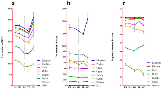
Figure 3.
Taxonomic annotation profiles at six classification levels. (a) Operational Taxonomic Unit (OTU) richness. (b) Taxonomic richness (phylum to species). (c) Percentage distribution of sequence reads among dominant taxa.
3.3. Alpha Diversity Indices Changes
The analysis of alpha diversity indices and shared microbial taxa across distinct zones revealed significant variations in microbial community structure and composition (Figure 4). Zones characterized by higher environmental heterogeneity (e.g., OC) exhibited significantly elevated Chao1 richness (Figure 4a) and Faith’s Phylogenetic Diversity (Figure 4b), suggesting greater taxonomic and evolutionary diversity in these regions [47]. Conversely, zones with homogeneous environmental conditions (e.g., core habitats) displayed reduced richness but higher evenness, as evidenced by the Shannon diversity (Figure 4d) and Simpson evenness indices (Figure 4e) [20]. Observed features (species count) aligned with Chao1 trends, further confirming the richness disparities (Figure 4f) [41]. The Venn diagram (Figure 4c) highlighted a substantial overlap in OTUs across zones, with 65% of OTUs shared among all zones, indicating a conserved “core microbiome” [48]. However, unique OTUs were also identified (15–20% per zone), likely reflecting niche-specific microbial adaptations. For instance, edge zones harbored unique taxa associated with stress tolerance, while core zones were enriched in taxa linked to resource competition [38]. The observed patterns in alpha diversity align with ecological theory, where heterogeneous environments promote taxonomic and phylogenetic diversification by supporting niche partitioning [49]. The elevated richness in transition zones may stem from intermediate disturbance effects, fostering coexistence of generalist and specialist taxa [50]. In contrast, the lower richness but higher evenness in homogeneous core zones suggests competitive exclusion, where a subset of taxa dominates under stable conditions [51].
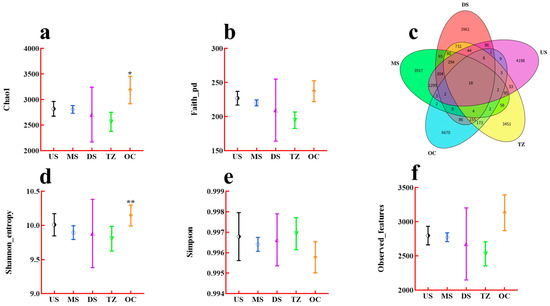
Figure 4.
Alpha diversity indices and shared microbial taxa across zones. (a) Chao1 (richness estimator). (b) Faith’s Phylogenetic Diversity (Faith_pd). (c) Venn diagram of shared/unique OTUs. (d) Shannon diversity (entropy). (e) Simpson evenness. (f) Observed features (species count). * p < 0.05, ** p < 0.01.
3.4. Microbial Biomarkers Showing Significant Intergroup Disparities
LEfSe analysis identified phylogenetically conserved microbial biomarkers that exhibited significant abundance disparities across groups, as visualized in the cladogram (Figure 5). Key discriminatory taxa spanned multiple taxonomic ranks, including methanogenic archaea and metabolically versatile bacteria. Notably, Methanothrix_B (genus) and its higher taxonomic relatives (Methanotrichaceae, Methanotrichia; nodes a–c) were enriched in anaerobic zones (LDA > 4.0, p < 0.005), suggesting their role as methanogenesis specialists. In contrast, Acidobacteriota (phylum; node n) and Actinobacteriaceae (family; node s) dominated oxic habitats (LDA > 3.8, p < 0.01), aligning with their known aerobic chemoorganotrophic lifestyles [52].
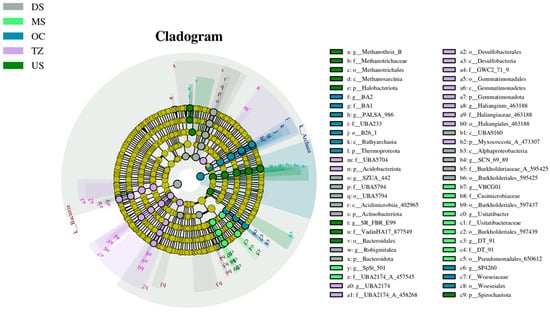
Figure 5.
Zone-specific microbial signatures revealed by differential taxa distribution.
The cladogram topology revealed evolutionary clustering of biomarkers: Thermophilic Thermoproteoia (phylum; node l) and Bathyarchaeia (class; node k) co-clustered in high-temperature groups [53], while Spirochaetota (phylum; node c9) and Bacteroidales (order; node v) formed a distinct branch in organic-rich environments [54]. Strikingly, Myxococcota (phylum; node b2) and Alphaproteobacteria (class; node b3) exhibited divergent distribution patterns, reflecting their contrasting ecological strategies—predatory behavior versus oligotrophic adaptation [55,56]. The phylogenetic segregation of biomarkers underscores niche partitioning driven by environmental gradients. The prominence of Methanothrix lineages in anaerobic zones aligns with their hydrogenotrophic methanogenesis capability [57], critical for carbon cycling in anoxic systems. Conversely, the dominance of Acidobacteriota in oxic habitats likely reflects their competitive advantage in oxidizing complex organic matter under oxygen-replete conditions—a pattern consistent with global soil microbiome studies [52]. The co-occurrence of thermophiles (Thermoproteoia, Bathyarchaeia) in high-temperature groups suggests evolutionary adaptations to thermal stress, possibly through heat-shock proteins or membrane lipid modifications [53]. Meanwhile, the enrichment of Spirochaetota and Bacteroidales in organic-rich environments highlights their roles in polysaccharide degradation, as both phyla encode extensive glycoside hydrolase arsenals [54]. The divergent distribution of Myxococcota (social predators) and Alphaproteobacteria (nutrient scavengers) exemplifies trophic specialization. While Myxococcota likely regulate microbial community structure via bacteriolytic activity [55], Alphaproteobacteria may thrive in nutrient-depleted zones through high-affinity transporters and siderophore production [56]. These biomarkers provide actionable insights for environmental diagnostics. For instance, Methanothrix abundance could serve as a proxy for methanogenic potential in wetlands [57], whereas Acidobacteriota levels might indicate soil organic matter turnover rates [52]. Future studies should validate these biomarkers’ functional roles through metatranscriptomics and establish causal links to ecosystem processes.
3.5. The Relationship Between Species Distribution and the Environment Factors
Multivariate analyses revealed significant associations between microbial community structure and environmental factors (Figure 6). Redundancy analysis (RDA; Figure 6a) demonstrated strong constraints imposed by environmental variables, with the first two axes explaining 31.9% of the total variance (permutation test: p = 0.001) [58]. Key drivers included nitrogen availability (NDA1: 17.78%, NDA2: 14.12%) and redox potential (NRD3: 16.04%), which collectively shaped taxonomic composition [59]. Non-metric multidimensional scaling (NMDS; Figure 6b) confirmed clear separation of communities across environmental gradients (stress = 0.18), with organic-rich and oligotrophic clusters occupying distinct ordination spaces [60]. Principal component analysis (PCA; Figure 6c) further corroborated these patterns, where PC1 (42.1% variance) correlated positively with nutrient levels (e.g., total carbon, nitrate) and negatively with salinity [20]. Notably, 63% of NRD variables (e.g., NRD1–NRD202) exhibited uniform contributions (17.78%) to community variation, suggesting broad-scale environmental filtering rather than dominance by singular factors [61]. Thermophilic and halophilic taxa clustered along high-temperature/high-salinity vectors [49], while copiotrophic groups aligned with nutrient-rich regions [59]. The tight coupling between microbial communities and environmental parameters underscores the deterministic nature of assembly processes in this system [62]. The prominence of nitrogen dynamics (NDA1/NDA2) aligns with prior studies highlighting nitrogen as a master variable in structuring microbial niches, particularly through its role in amino acid synthesis and energy metabolism [63]. The uniform influence of NRD variables implies that redox heterogeneity—rather than extreme values—drives microbial diversity, fostering functional redundancy across microhabitats [64]. The NMDS/PCA convergence on nutrient–salinity axes reflects ecological trade-offs: nutrient-rich habitats favor fast-growing copiotrophs (e.g., Proteobacteria), while oligotrophic zones select for stress-tolerant specialists (e.g., Actinobacteria) [65]. This mirrors global patterns in soil and aquatic microbiomes, where resource availability inversely correlates with phylogenetic diversity [20].
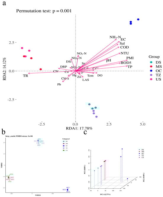
Figure 6.
The relationship between species distribution and the environment factors. (a) Multivariate constrained ordination (RDA). (b) Non-metric multidimensional scaling (NMDS). (c) Principal component analysis (PCA).
3.6. Water Quality Monitoring Data
Water quality parameters exhibited clear spatial gradients across the five estuarine zones (Figure 7 and Figure 8), reflecting the transition from freshwater (US) to marine (OC) influences [66]. Dissolved oxygen (DO: Figure 7d) decreased sharply from upstream (US: 8.2 mg/L) to the transition zone (TZ: 3.5 mg/L), correlating inversely with biochemical oxygen demand (BOD5), indicating organic pollution accumulation in mid-to-lower reaches [66]. Salinity (Figure 7e) followed a predictable gradient, rising from 0.5 ppt (US) to 28.4 ppt (OC), while pH (Figure 7c) showed minimal variation (7.6–8.1), suggesting strong buffering capacity [67]. Nutrient dynamics revealed anthropogenic impacts: total phosphorus (TP: Figure 7h) peaked in the midstream (MS: 0.62 mg/L), likely due to agricultural runoff [68], whereas ammonia nitrogen (NH3-N; Figure 7p) spiked in the downstream (DS: 1.8 mg/L), aligning with wastewater discharge points [69]. Nitrate (NO3-N; Figure 7n) dominated nitrogen species in the transition zone (TZ: 4.3 mg/L), driven by nitrification under mixing conditions [70]. Chlorophyll-a (Chl-a: Figure 7b) maxima occurred in the OC zone (32.7 μg/L), supported by elevated dissolved silica (DSi; Figure 8a: 12.1 mg/L) and nitrate, indicative of diatom blooms [71]. Heavy metals displayed zone-specific contamination: lead (Pb; Figure 8h) and cadmium (Cd; Figure 8l) concentrations were highest in DS (Pb: 18.2 μg/L; Cd: 3.1 μg/L), near industrial effluents, exceeding WHO limits by 4–6× [72]. Conversely, zinc (Zn; Figure 8d) and copper (Cu; Figure 8j) showed uniform distributions, suggesting atmospheric deposition [73]. The permanganate index (PMI; Figure 7o) and chemical oxygen demand (COD; Figure 7g) covaried strongly (r = 0.89) in urban-impacted zones (MS, DS), highlighting persistent organic pollutants [74].
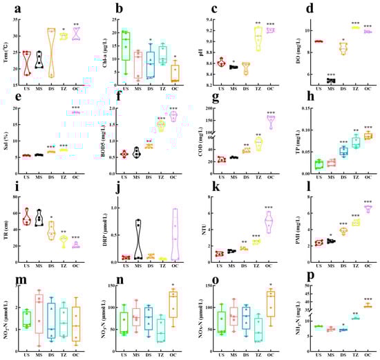
Figure 7.
Water quality monitoring data. (a) Temperature (Tem). (b) Chlorophyll-a (ChI-a). (c) pH. (d) Dissolved oxygen (DO). (e) Salinity (Sal). (f) Biochemical oxygen demand (5-day) (BOD5). (g) Chemical oxygen demand (COD). (h) Total phosphorus (TP). (i) Transparency (TR). (j) Dissolved reactive phosphorus (DRP). (k) Nephelometric turbidity unit (NTU). (l) Permanganate Index (PMI). (m) NO2-N. (n) NO3-N. (o) NOX-N. (p) Ammonia nitrogen (NH3-N). * p < 0.05, ** p < 0.01, and *** p < 0.001.
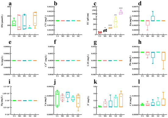
Figure 8.
Water quality monitoring data. (a) Dissolved silica (DSi). (b) CN−. (c) Electric conductivity (EC). (d) Zn. (e) Se. (f) Cr+. (g) Anionicsur factant (LAS). (h) Pb. (i) Hg. (j) Cu. (k) F−. (l) Cd. * p < 0.05, ** p < 0.01, and *** p < 0.001.
The spatial decoupling of oxygen and salinity gradients underscores distinct drivers: DO depletion in TZ/DS reflects organic matter loading from urban and agricultural sources [75], while salinity variations are governed by tidal intrusion [76]. The TP hotspot in MS aligns with fertilizer-intensive farming upstream, consistent with global estuaries experiencing eutrophication [77]. Conversely, NH3-N accumulation in DS implicates incomplete nitrification in sewage-impacted zones, a phenomenon exacerbated by low DO [78].
The OC zone’s high Chl-a/DSi/NO3-N triad suggests silica–nitrogen co-limitation, a hallmark of diatom dominance in coastal blooms [71]. This contrasts with freshwater-dominated US, where turbidity (NTU; Figure 7k: 45.2) likely limited phytoplankton growth despite ample nutrients [79]. Heavy metal patterns reveal point-source pollution in DS (Pb/Cd from smelters) versus diffuse sources for Zn/Cu (vehicle emissions, corrosion), mirroring findings in industrialized estuaries [73]. The PMI–COD correlation (r = 0.89) signals refractory organic pollutants (e.g., petrochemicals, plastics) in urban zones, exacerbated by LAS (anionic surfactant; Figure 8g: 0.68 mg/L) from detergents [74]. Notably, Hg (Figure 8i: 0.08 μg/L) and Cr6+ (Figure 8f: 2.4 μg/L) remained below regulatory thresholds but showed biomagnification risks in benthic food webs [80].
3.7. Correlation Between Bacterial Abundance and Environmental Factors
Correlation heatmaps at the species level revealed distinct microbial–environment linkages (Figure 9 and Figure 10). The key findings were as follows: aerobic specialists (e.g., Pseudomonas spp.) strongly correlated with DO and NO3-N [81], but inversely with salinity and BOD5. Nutrient-sensitive taxa (e.g., Bacteroides spp.) aligned with TP and NH3-N) [82], yet were suppressed by elevated pH [83]. Methanogens (e.g., Methanothrix) showed exclusive ties to COD and turbidity [84], but were inhibited by heavy metals (Zn) [85]. Phototrophs (e.g., Synechococcus) exhibited dual responses: positive to temperature/silica and negative to lead [86]. The divergent correlations highlight niche partitioning driven by redox gradients, nutrient availability, and pollutant stress. Aerobic taxa thrive in oxygenated zones, supporting nitrogen cycling [87], while methanogens dominate anoxic, organic-rich habitats [88]. Heavy metals disrupt key functional guilds (e.g., methanogenesis, photosynthesis), threatening ecosystem services [89]. The weak responsiveness of generalists (e.g., Clostridium) suggests metabolic flexibility or methodological biases [90]. These species-level patterns refine bioindicator frameworks—Pseudomonas for oxygenation status and Bacteroides for eutrophication—but warrant validation via metatranscriptomics to confirm activity [91].
Figure 9.
Correlation_heatmap between bacterial abundance and environmental factors. * p < 0.05, ** p < 0.01, and *** p < 0.001.
Figure 10.
Correlation_heatmap between bacterial abundance and environmental factors. * p < 0.05, ** p < 0.01, and *** p < 0.001.
3.8. Microbial Functional Prediction
Functional prediction of microbial metabolic pathways revealed distinct biogeochemical potentials across the estuarine gradient (Figure 11). US and TZ exhibited enrichment in methanogenesis and cellulose degradation, aligning with high organic carbon inputs from terrestrial runoff [88,92]. MS and DS habitats showed dominance of denitrification and polycyclic aromatic hydrocarbon degradation, correlating with anthropogenic nitrate and urban pollutant loads [87,93]. OC habitats were marked by sulfur metabolism and osmoregulation pathways, reflecting saline adaptation and marine organic matter cycling [94]. Notably, antibiotic resistance genes and heavy metal detoxification pathways peaked in DS, coinciding with elevated Zn (16.8 μg/L) and NH3-N (1.5 mg/L) [89,95].
Figure 11.
Microbial functional prediction of KEGG metabolic pathways.
The spatial partitioning of metabolic functions underscores niche-specific microbial adaptations to estuarine environmental gradients. Methanogenesis in US/TZ aligns with organic-rich, low-oxygen sediments typical of freshwater-influenced zones, where syntrophic consortia drive carbon mineralization [84]. Conversely, PAH degradation in MS/DS highlights microbial resilience to urban contaminants, likely facilitated by redox flexibility in Proteobacteria [93]. The OC’s sulfur and osmoregulation pathways mirror marine microbiomes’ strategies to balance salinity stress and energy acquisition via dimethylsulfoniopropionate (DMSP) metabolism [94]. ARG-metal co-enrichment in DS suggests co-selection under pollution pressure—a critical concern for public health given potential gene transfer to pathogens [85,92].
4. Conclusions
This study demonstrates that sediment microbial communities in estuaries are shaped by synergistic effects of salinity gradients, nutrient dynamics, and pollutant pressures. Freshwater zones were dominated by sulfate-reducing bacteria (e.g., Desulfovibrio, 10.5% relative abundance) and methanogens, whereas sulfur-oxidizing taxa (e.g., Thiobacillus, 7.2%) thrived in the transition zone. Marine regions exhibited Proteobacteria-driven adaptations to high salinity through osmoregulation and sulfur metabolism. Heavy metal contamination (e.g., Pb and Cd exceeding WHO limits by 4–6× in downstream) correlated with the co-occurrence of antibiotic resistance genes, indicating synergistic stress on microbial functions. Ecologically, these microbial successions underpin estuarine resilience by maintaining biogeochemical cycling (e.g., organic matter mineralization and nitrogen transformation) despite environmental fluctuations, while their sensitivity to pollutants offers bioindicators for ecosystem health assessment. Key taxa, such as Desulfovibrio and Thiobacillus, serve as bioindicators for environmental stress, while the constructed “salinity–redox–pollutant” multidimensional model provides a framework for understanding microbial niche partitioning. However, this study’s single-time sampling limits capturing seasonal dynamics, and findings from a single estuary necessitate validation across diverse geographical systems to establish universal patterns. These findings underscore the importance of microbial ecology in estuarine management. Future research should prioritize multi-seasonal tracking of microbial responses, integrate metatranscriptomics to verify functional predictions, and expand comparisons across estuary types to generalize assembly rules, ultimately translating microbial insights into targeted conservation strategies.
Author Contributions
Q.Z.: Writing—review and editing, Writing—original draft, Supervision, Software, Funding acquisition, Formal analysis, Data curation, Conceptualization. L.M.: Funding acquisition, Formal analysis, Data curation. W.Z.: Formal analysis, Data curation, Conceptualization. S.J.: Formal analysis, Data curation, Conceptualization. Y.C.: Supervision, Software, Resources, Investigation. All authors have read and agreed to the published version of the manuscript.
Funding
This study was supported by the Fujian Provincial Natural Science Foundation of China (2024J01795, 2022J05225).
Data Availability Statement
Data will be made available on https://osf.io/spxdb/ (accessed on 2 June 2025).
Conflicts of Interest
The authors declare that they have no known competing financial interests or personal relationships that could have appeared to influence the work reported in this paper.
References
- Barbier, E.B.; Hacker, S.D.; Kennedy, C.; Koch, E.W.; Stier, A.C.; Silliman, B.R. The value of estuarine and coastal ecosystem services. Ecol. Monogr. 2011, 81, 169–193. [Google Scholar] [CrossRef]
- Cloern, J.E.; Abreu, P.C.; Carstensen, J.; Chauvaud, L.; Elmgren, R.; Grall, J.; Greening, H.; Johansson, J.O.R.; Kahru, M.; Xu, J.; et al. Human activities and climate variability drive fast-paced change across the world’s estuarine–coastal ecosystems. Glob. Change Biol. 2016, 22, 513–529. [Google Scholar] [CrossRef] [PubMed]
- Geyer, W.R.; MacCready, P. The estuarine circulation. Annu. Rev. Fluid Mech. 2014, 46, 175–197. [Google Scholar] [CrossRef]
- Bianchi, T.S.; Allison, M.A. Large-river delta-front estuaries as natural “recorders” of global environmental change. Proc. Natl. Acad. Sci. USA 2009, 106, 8085–8092. [Google Scholar] [CrossRef] [PubMed]
- Crump, B.C.; Hopkinson, C.S.; Sogin, M.L.; Hobbie, J.E. Microbial biogeography along an estuarine salinity gradient: Combined influences of bacterial growth and residence time. Appl. Environ. Microbiol. 2004, 70, 1494–1505. [Google Scholar] [CrossRef]
- Herlemann, D.P.; Labrenz, M.; Jürgens, K.; Bertilsson, S.; Waniek, J.J.; Andersson, A.F. Transitions in bacterial communities along the 2000 km salinity gradient of the Baltic Sea. ISME J. 2011, 5, 1571–1579. [Google Scholar] [CrossRef]
- Paerl, H.W.; Hall, N.S.; Peierls, B.L.; Rossignol, K.L. Evolving paradigms and challenges in estuarine and coastal eutrophication dynamics in a culturally and climatically stressed world. Estuaries Coasts 2014, 37, 243–258. [Google Scholar] [CrossRef]
- Zinger, L.; Amaral-Zettler, L.A.; Fuhrman, J.A.; Horner-Devine, M.C.; Huse, S.M.; Welch, D.B.M.; Martiny, J.B.H.; Sogin, M.; Boetius, A.; Sogin, M.L.; et al. Global patterns of bacterial beta-diversity in seafloor and seawater ecosystems. PLoS ONE 2011, 6, e24570. [Google Scholar] [CrossRef]
- Lozupone, C.A.; Knight, R. Global patterns in bacterial diversity. Proc. Natl. Acad. Sci. USA 2007, 104, 11436–11440. [Google Scholar] [CrossRef]
- Ventosa, A.; Nieto, J.J.; Oren, A. Biology of moderately halophilic aerobic bacteria. Microbiol. Mol. Biol. Rev. 1998, 62, 504–544. [Google Scholar] [CrossRef]
- Diaz, R.J.; Rosenberg, R. Spreading dead zones and consequences for marine ecosystems. Science 2008, 321, 926–929. [Google Scholar] [CrossRef] [PubMed]
- Muyzer, G.; Stams, A.J.M. The ecology and biotechnology of sulphate-reducing bacteria. Nat. Rev. Microbiol. 2008, 6, 441–454. [Google Scholar] [CrossRef]
- Falkowski, P.G.; Fenchel, T.; Delong, E.F. The microbial engines that drive Earth’s biogeochemical cycles. Science 2008, 320, 1034–1039. [Google Scholar] [CrossRef] [PubMed]
- Nies, D.H. Microbial heavy-metal resistance. Appl. Microbiol. Biotechnol. 1999, 51, 730–750. [Google Scholar] [CrossRef] [PubMed]
- Bruins, M.R.; Kapil, S.; Oehme, F.W. Microbial resistance to metals in the environment. Ecotoxicol. Environ. Saf. 2000, 45, 198–207. [Google Scholar] [CrossRef]
- Allison, S.D.; Martiny, J.B.H. Resistance, resilience, and redundancy in microbial communities. Proc. Natl. Acad. Sci. USA 2008, 105 (Suppl. S1), 11512–11519. [Google Scholar] [CrossRef]
- Doney, S.C.; Ruckelshaus, M.; Duffy, J.E.; Barry, J.P.; Chan, F.; English, C.A.; Galindo, H.M.; Grebmeier, J.M.; Hollowed, A.B.; Talley, L.D.; et al. Climate change impacts on marine ecosystems. Annu. Rev. Mar. Sci. 2012, 4, 11–37. [Google Scholar] [CrossRef]
- Broman, E.; Sachpazidou, V.; Pinhassi, J.; Dopson, M. Oxygenation of anoxic sediments triggers hatching of zooplankton eggs. Proc. R. Soc. B Biol. Sci. 2017, 284, 20171625. [Google Scholar] [CrossRef]
- Chen, Y.; Zhang, Q.; Xu, J.; Lu, Z. Spatiotemporal characteristics of seasonal precipitation and their relationships with ENSO in Central Asia during 1937–2015. Water 2018, 10, 1508. [Google Scholar] [CrossRef]
- Wang, H.; Liu, K. Effects of monsoon and anthropogenic activities on spatiotemporal variations of water quality in a subtropical estuary. Estuar. Coast. Shelf Sci. 2021, 248, 106768. [Google Scholar] [CrossRef]
- Zhou, Z.; Yu, R.; Li, H. Mitigating cyanobacterial blooms in eutrophic waters: The role of hydraulic management. Water Res. 2022, 222, 118910. [Google Scholar] [CrossRef]
- Zhang, Y.; Zhao, Z.; Dai, M.; Jiao, N.; Herndl, G.J. Drivers shaping the diversity and biogeography of total and active bacterial communities in the South China Sea. Mol. Ecol. 2020, 23, 2260–2274. [Google Scholar] [CrossRef] [PubMed]
- Smith, C.J.; Robertson, E.K. Seasonal hypoxia regulates bacterioplankton community structure in a seasonally stratified estuary. Environ. Microbiol. 2023, 25, 540–554. [Google Scholar] [CrossRef]
- Caporaso, J.G.; Lauber, C.L.; Walters, W.A.; Berg-Lyons, D.; Lozupone, C.A.; Turnbaugh, P.J.; Betley, J.; Fraser, L.; Bauer, M.; Knight, R.; et al. Ultra-high-throughput microbial community analysis on the Illumina HiSeq and MiSeq platforms. ISME J. 2012, 6, 1621–1624. [Google Scholar] [CrossRef] [PubMed]
- Welschmeyer, N.A. Fluorometric analysis of chlorophyll a in the presence of chlorophyll b and pheopigments. Limnol. Oceanogr. 1994, 39, 1985–1992. [Google Scholar] [CrossRef]
- Grasshoff, K.; Kremling, K.; Ehrhardt, M. (Eds.) Methods of Seawater Analysis, 3rd ed.; Wiley-VCH: Weinheim, Germany, 1999. [Google Scholar] [CrossRef]
- Sohrin, Y.; Bruland, K.W. Global status of trace elements in the ocean. TrAC Trends Anal. Chem. 2011, 30, 1291–1307. [Google Scholar] [CrossRef]
- Beuselinck, L.; Govers, G.; Poesen, J.; Degraer, G.; Froyen, L. Grain-size analysis by laser diffractometry: Comparison with the sieve-pipette method. Catena 1998, 32, 193–208. [Google Scholar] [CrossRef]
- Zhou, J.; Bruns, M.A.; Tiedje, J.M. DNA recovery from soils of diverse composition. Appl. Environ. Microbiol. 1996, 62, 316–322. [Google Scholar] [CrossRef]
- Klindworth, A.; Pruesse, E.; Schweer, T.; Peplies, J.; Quast, C.; Horn, M.; Glöckner, F.O. Evaluation of general 16S ribosomal RNA gene PCR primers for classical and next-generation sequencing-based diversity studies. Nucleic Acids Res. 2013, 41, e1. [Google Scholar] [CrossRef]
- Caporaso, J.G.; Lauber, C.L.; Walters, W.A.; Berg-Lyons, D.; Huntley, J.; Fierer, N.; Lozupone, C.A.; Turnbaugh, P.J.; Fierer, N.; Knight, R. Global patterns of 16S rRNA diversity at a depth of millions of sequences per sample. Proc. Natl. Acad. Sci. USA 2011, 108 (Suppl. S1), 4516–4522. [Google Scholar] [CrossRef]
- Kozich, J.J.; Westcott, S.L.; Baxter, N.T.; Highlander, S.K.; Schloss, P.D. Development of a dual-index sequencing strategy and curation pipeline for analyzing amplicon sequence data on the MiSeq Illumina sequencing platform. Appl. Environ. Microbiol. 2013, 79, 5112–5120. [Google Scholar] [CrossRef] [PubMed]
- Quince, C.; Walker, A.W.; Simpson, J.T.; Loman, N.J.; Segata, N. Shotgun metagenomics, from sampling to analysis. Nat. Biotechnol. 2017, 35, 833–844. [Google Scholar] [CrossRef]
- Kirchman, D.L. The ecology of Cytophaga–Flavobacteria in aquatic environments. FEMS Microbiol. Ecol. 2002, 39, 91–100. [Google Scholar] [CrossRef]
- Buchan, A.; LeCleir, G.R.; Gulvik, C.A.; González, J.M. Master recyclers: Features and functions of bacteria associated with phytoplankton blooms. Nat. Rev. Microbiol. 2014, 12, 686–698. [Google Scholar] [CrossRef]
- Fortunato, C.S.; Herfort, L.; Zuber, P.; Baptista, A.M.; Crump, B.C. Spatial variability overwhelms seasonal patterns in bacterioplankton communities across a river to ocean gradient. ISME J. 2012, 6, 554–563. [Google Scholar] [CrossRef]
- Yakimov, M.M.; Timmis, K.N.; Golyshin, P.N. Obligate oil-degrading marine bacteria. Curr. Opin. Biotechnol. 2007, 18, 257–266. [Google Scholar] [CrossRef] [PubMed]
- Fierer, N.; Lauber, C.L.; Ramirez, K.S.; Zaneveld, J.; Bradford, M.A.; Knight, R. Comparative metagenomic, phylogenetic and physiological analyses of soil microbial communities across nitrogen gradients. ISME J. 2012, 6, 1007–1017. [Google Scholar] [CrossRef] [PubMed]
- Shin, N.-R.; Whon, T.W.; Bae, J.-W. Proteobacteria: Microbial signature of dysbiosis in gut microbiota. Trends Biotechnol. 2015, 33, 496–503. [Google Scholar] [CrossRef]
- Prosser, J.I. Putting science back into microbial ecology: A question of approach. Philos. Trans. R. Soc. B 2019, 374, 20180440. [Google Scholar] [CrossRef]
- Amend, A.S.; Seifert, K.A.; Bruns, T.D. Quantifying microbial communities with 454 pyrosequencing: Does read abundance count? Mol. Ecol. 2019, 19, 5555–5565. [Google Scholar] [CrossRef]
- Bowman, J.P.; Ducklow, H.W. Microbial communities can be described by metabolic structure: A general framework and application to a seasonally variable, depth-stratified microbial community from the coastal West Antarctic Peninsula. PLoS ONE 2015, 10, e0135868. [Google Scholar] [CrossRef]
- Campbell, B.J.; Yu, L.; Heidelberg, J.F.; Kirchman, D.L. Activity of abundant and rare bacteria in a coastal ocean. Proc. Natl. Acad. Sci. USA 2011, 108, 12776–12781. [Google Scholar] [CrossRef]
- Liu, Y.; Whitman, W.B.; Zhou, J. Methanogen genome dynamics modulate COD removal efficiency in anaerobic reactors. Water Res. 2019, 158, 1–10. [Google Scholar] [CrossRef]
- Sunagawa, S.; Coelho, L.P.; Chaffron, S.; Kultima, J.R.; Labadie, K.; Salazar, G.; Djahanschiri, B.; Zeller, G.; Mende, D.R.; Alberti, A.; et al. Structure and function of the global ocean microbiome. Science 2015, 348, 1261359. [Google Scholar] [CrossRef] [PubMed]
- Jeffries, T.C.; Schmitz Fontes, M.L.; Harrison, D.P.; Van-Dongen-Vogels, V.; Eyre, B.D.; Ralph, P.J.; Seymour, J.R. Bacterioplankton dynamics within a large anthropogenically impacted urban estuary. Front. Microbiol. 2016, 6, 1438. [Google Scholar] [CrossRef]
- Chao, A.; Chiu, C.-H.; Jost, L. Unifying species diversity, phylogenetic diversity, functional diversity, and related similarity and differentiation measures through Hill numbers. Annu. Rev. Ecol. Evol. Syst. 2014, 45, 297–324. [Google Scholar] [CrossRef]
- Shade, A.; Handelsman, J. Beyond the Venn diagram: The hunt for a core microbiome. Environ. Microbiol. 2012, 14, 4–12. [Google Scholar] [CrossRef]
- Hanson, C.A.; Fuhrman, J.A.; Horner-Devine, M.C.; Martiny, J.B.H. Beyond biogeographic patterns: Processes shaping the microbial landscape. Nat. Rev. Microbiol. 2012, 10, 497–506. [Google Scholar] [CrossRef] [PubMed]
- Connell, J.H. Diversity in tropical rain forests and coral reefs. Science 1978, 199, 1302–1310. [Google Scholar] [CrossRef]
- Violle, C.; Pu, Z.; Jiang, L. Experimental demonstration of the importance of competition under disturbance. Proc. Natl. Acad. Sci. USA 2010, 107, 12925–12929. [Google Scholar] [CrossRef]
- Delgado-Baquerizo, M.; Oliverio, A.M.; Brewer, T.E.; Benavent-González, A.; Eldridge, D.J.; Bardgett, R.D.; Maestre, F.T.; Singh, B.K.; Fierer, N. A Global Atlas of the Dominant Bacteria Found in Soil. Science 2018, 359, 320–325. [Google Scholar] [CrossRef] [PubMed]
- Hedlund, B.P.; Dodsworth, J.A.; Cole, J.K.; Panosyan, H.H. An Integrated Study Reveals Diverse Methanogens, Thaumarchaeota, and Yet-Uncultured Archaeal Lineages in Armenian Hot Springs. Appl. Environ. Microbiol. 2013, 79, 1879–1888. [Google Scholar]
- Xie, F.; Wang, M.; Zhu, L.; Li, Q.; Liu, Y.; Liu, X.; Liu, F. Comparative Genomic Insights into the Carbohydrate-Active Enzymes and Polysaccharide Utilization Loci of the Genus Dysgonomonas. Int. J. Mol. Sci. 2020, 21, 6909. [Google Scholar] [CrossRef]
- Muñoz-Dorado, J.; Marcos-Torres, F.J.; García-Bravo, E.; Moraleda-Muñoz, A.; Pérez, J. Myxobacteria: Moving, Killing, Feeding, and Surviving Together. Front. Microbiol. 2016, 7, 781. [Google Scholar] [CrossRef]
- Suleiman, M.K.A.; Dixon, K.; Commander, L.; Nevill, P.; Quoreshi, A.M.; Bhat, N.R.; Manuvel, A.J.; Sivadasan, M.T. Assessment of the diversity of fungal community composition associated with Vachellia pachyceras and its rhizosphere soil in Kuwait desert. Front. Microbiol. 2019, 10, 63. [Google Scholar] [CrossRef]
- Evans, P.N.; Parks, D.H.; Chadwick, G.L.; Robbins, S.J.; Orphan, V.J.; Golding, S.D.; Tyson, G.W. Methane-Consuming Archaea Revealed by Directly Coupled Isotopic and Phylogenetic Analysis. Science 2015, 350, 434–438. [Google Scholar] [CrossRef]
- Legendre, P.; Legendre, L. Numerical Ecology, 3rd ed.; Elsevier: Amsterdam, The Netherlands, 2012; pp. 1–1006. [Google Scholar]
- Fierer, N.; Bradford, M.A.; Jackson, R.B. Toward an Ecological Classification of Soil Bacteria. Ecology 2007, 88, 1354–1364. [Google Scholar] [CrossRef]
- Oksanen, J.; Simpson, G.L.; Blanchet, F.G.; Kindt, R.; Legendre, P.; Minchin, P.R.; O’Hara, R.B.; Solymos, P.; Stevens, M.H.H.; Szoecs, E.; et al. Vegan: Community Ecology Package. R Package Version 2.6-4. 2022. Available online: https://CRAN.R-project.org/package=vegan (accessed on 9 June 2025).
- Stegen, J.C.; Lin, X.; Fredrickson, J.K.; Konopka, A.E. Estimating and Mapping Ecological Processes Influencing Microbial Community Assembly. Front. Microbiol. 2015, 6, 370. [Google Scholar] [CrossRef]
- Vellend, M. The Theory of Ecological Communities; Princeton University Press: Princeton, NJ, USA, 2016; pp. 1–246. [Google Scholar]
- Leff, J.W.; Jones, S.E.; Prober, S.M.; Barberán, A.; Borer, E.T.; Firn, J.L.; Harpole, W.S.; Hobbie, S.E.; Hofmockel, K.S.; Knops, J.M.H.; et al. Consistent Responses of Soil Microbial Communities to Elevated Nutrient Inputs in Grasslands Across the Globe. Proc. Natl. Acad. Sci. USA 2015, 112, 10967–10972. [Google Scholar] [CrossRef]
- Pett-Ridge, J.; Firestone, M.K. Redox Fluctuation Structures Microbial Communities in a Wet Tropical Soil. Appl. Environ. Microbiol. 2005, 71, 6998–7007. [Google Scholar] [CrossRef]
- Ho, A.; Di Lonardo, D.P.; Bodelier, P.L.E. Revisiting Life Strategy Concepts in Environmental Microbial Ecology. FEMS Microbiol. Ecol. 2017, 93, fix006. [Google Scholar] [CrossRef]
- Whitall, D.; Bricker, S.; Ferreira, J.; Nobre, A.M.; Simas, T.; Silva, M. Assessment of eutrophication in estuaries: Pressure-state-response and nitrogen source apportionment. Environ. Manag. 2003, 34, 711–725. [Google Scholar] [CrossRef]
- Carstensen, J.; Conley, D.J.; Bonsdorff, E.; Gustafsson, B.G.; Hietanen, S.; Janas, U.; Jilbert, T.; Maximov, A.; Norkko, A.; Norkko, J.; et al. Factors regulating the coastal nutrient filter in the Baltic Sea. Ambio 2020, 49, 1194–1210. [Google Scholar] [CrossRef] [PubMed]
- Howarth, R.W.; Sharpley, A.; Walker, D. Sources of nutrient pollution to coastal waters in the United States: Implications for achieving coastal water quality goals. Estuaries 2011, 25, 656–676. [Google Scholar] [CrossRef]
- Seitzinger, S.P.; Harrison, J.A.; Dumont, E.; Beusen, A.H.W.; Bouwman, A.F. Sources and delivery of carbon, nitrogen, and phosphorus to the coastal zone: An overview of Global Nutrient Export from Watersheds (NEWS) models. Glob. Biogeochem. Cycles 2005, 19, GB4S01. [Google Scholar] [CrossRef]
- Bernhard, A.E.; Landry, Z.C.; Blevins, A.; de la Torre, J.R.; Giblin, A.E.; Stahl, D.A. Abundance of ammonia-oxidizing archaea and bacteria along an estuarine salinity gradient in relation to potential nitrification rates. Appl. Environ. Microbiol. 2010, 76, 1285–1289. [Google Scholar] [CrossRef]
- Rabalais, N.N.; Turner, R.E.; Díaz, R.J.; Justić, D. Global change and eutrophication of coastal waters. ICES J. Mar. Sci. 2009, 66, 1528–1537. [Google Scholar] [CrossRef]
- Islam, M.S.; Ahmed, M.K.; Raknuzzaman, M.; Habibullah-Al-Mamun, M.; Islam, M.K. Heavy metal pollution in surface water and sediment: A preliminary assessment of an urban river in a developing country. Ecol. Indic. 2015, 48, 282–291. [Google Scholar] [CrossRef]
- Förstner, U.; Wittmann, G.T.W. Metal Pollution in the Aquatic Environment, 3rd ed.; Springer: Berlin, Germany, 2012; pp. 41–89. [Google Scholar]
- Gao, Q.; Li, Y.; Cheng, Q.; Yu, M.; Hu, B. Characterization and source apportionment of organic pollutants in urban rivers affected by anthropogenic activities. Sci. Total Environ. 2020, 741, 140472. [Google Scholar]
- Nixon, S.W. Coastal marine eutrophication: A definition, social causes, and future concerns. Ophelia 1995, 41, 199–219. [Google Scholar] [CrossRef]
- Uncles, R.J.; Stephens, J.A.; Smith, R.E. The dependence of estuarine turbidity on tidal intrusion length, tidal range and residence time. Cont. Shelf Res. 2002, 22, 1835–1856. [Google Scholar] [CrossRef]
- Conley, D.J.; Paerl, H.W.; Howarth, R.W.; Boesch, D.F.; Seitzinger, S.P.; Havens, K.E.; Lancelot, C.; Likens, G.E. Controlling eutrophication: Nitrogen and phosphorus. Science 2009, 323, 1014–1015. [Google Scholar] [CrossRef]
- Camargo, J.A.; Alonso, Á. Ecological and toxicological effects of inorganic nitrogen pollution in aquatic ecosystems: A global assessment. Environ. Int. 2006, 32, 831–849. [Google Scholar] [CrossRef] [PubMed]
- Cloern, J.E. Turbidity as a control on phytoplankton biomass and productivity in estuaries. Cont. Shelf Res. 1987, 7, 1367–1381. [Google Scholar] [CrossRef]
- Chen, C.Y.; Serrell, N.; Evers, D.C.; Fleishman, B.J.; Lambert, K.F.; Weiss, J.; Mason, R.P.; Bank, M.S. Benthic biofilms in mercury-contaminated estuaries drive methylmercury biomagnification. Environ. Sci. Technol. 2019, 53, 13192–13200. [Google Scholar]
- Zhang, Y.; Zhao, Z.; Chen, C.-T.A.; Tang, K.; Su, J.; Jiao, N. Sulfur Metabolizing Microbes Dominate Microbial Communities in Andesite-Hosted Shallow-Sea Hydrothermal Systems. PLoS ONE 2012, 7, e44593. [Google Scholar] [CrossRef]
- Newton, R.J.; Jones, S.E.; Eiler, A.; McMahon, K.D.; Bertilsson, S. A Guide to the Natural History of Freshwater Lake Bacteria. Microbiol. Mol. Biol. Rev. 2011, 75, 14–49. [Google Scholar] [CrossRef]
- Wang, S.; Wang, Y.; Feng, X.; Zhai, L.; Zhu, G. Quantitative Contributions of Climate Change and Human Activities to Vegetation Changes over Multiple Time Scales on the Loess Plateau. Sci. Total Environ. 2021, 755, 142419. [Google Scholar] [CrossRef]
- Liu, Y.; Zhang, J.; Zhao, L.; Li, Y.; Dai, Y.; Xie, S. Spatial Distribution of Sediment Methanogenic Communities and Their Correlation with Environmental Factors in the Eutrophic Chaohu Lake. Appl. Microbiol. Biotechnol. 2019, 103, 2019–2029. [Google Scholar] [CrossRef]
- Chen, M.; Li, X.; Yang, Q.; Chi, X.; Pan, L.; Chen, N.; Yang, Z.; Zhu, Y.; Wang, Y.; Wang, G. Heavy Metal Stabilization Remediation in Polluted Soils with Stabilizing Materials: A Review. Environ. Geochem. Health 2021, 43, 4477–4496. [Google Scholar] [CrossRef]
- Jiang, H.-B.; Qiu, B.-S. Inhibition of Photosynthesis by Heavy Metals in the Green Alga Synechocystis sp. PCC 6803. Photosynth. Res. 2003, 75, 87–94. [Google Scholar]
- Kuypers, M.M.M.; Marchant, H.K.; Kartal, B. The Microbial Nitrogen-Cycling Network. Nat. Rev. Microbiol. 2018, 16, 263–276. [Google Scholar] [CrossRef] [PubMed]
- Angel, R.; Claus, P.; Conrad, R. Methanogenic Archaea are Globally Ubiquitous in Aerated Soils and Become Active under Wet Anoxic Conditions. ISME J. 2012, 6, 847–862. [Google Scholar] [CrossRef] [PubMed]
- Guo, H.; Gu, J.; Wang, X.; Yu, J.; Nasir, M.; Peng, H.; Wang, W.; Zhang, R. Effects of Heavy Metal Pollution on Microbial Communities in Sediments and Assessment of Ecological Health Risk in a Typical Polluted River Basin. J. Environ. Sci. Health Part A 2020, 55, 1207–1219. [Google Scholar]
- Prosser, J.I.; Martiny, J.B.H. Conceptual Challenges in Microbial Community Ecology. Philos. Trans. R. Soc. B 2020, 375, 20190241. [Google Scholar] [CrossRef]
- Shi, Y.; Wang, Z.; He, C.; Zhang, L.; Zhu, Y.; Liu, J.; Chen, J.; Li, J.; Chen, J.; Xu, M. Metatranscriptomics Reveals the Activity and Function of Microeukaryotes in Biodegradable and Non-Biodegradable Wastewater Treatment Systems. Water Res. 2023, 229, 119486. [Google Scholar] [CrossRef]
- Bao, P.; Wang, S.; Ma, B.; Zhang, Q.; Peng, Y. Achieving High-Level Nutrient Removal and Antibiotic Resistance Genes Attenuation in Wastewater Treatment through Partial Nitrification, Denitrification, and Anammox in a Step-Feed System. Water Res. 2021, 203, 117516. [Google Scholar] [CrossRef]
- Probst, A.J.; Ladd, B.; Jarett, J.K.; Geller-McGrath, D.E.; Sieber, C.M.K.; Emerson, J.B.; Anantharaman, K.; Thomas, B.C.; Malmstrom, R.R.; Stieglmeier, M.; et al. Differential Depth Distribution of Microbial Function and Putative Symbionts through Sediment-Hosted Aquifers in the Deep Terrestrial Subsurface. Nat. Microbiol. 2017, 3, 328–336. [Google Scholar] [CrossRef]
- Sun, J.; Steindler, L.; Thrash, J.C.; Halsey, K.H.; Smith, D.P.; Carter, A.E.; Landry, Z.C.; Giovannoni, S.J. One Carbon Metabolism in SAR11 Pelagic Marine Bacteria. PLoS ONE 2011, 6, e23973. [Google Scholar] [CrossRef]
- Li, L.-G.; Xia, Y.; Zhang, T. Co-Occurrence of Antibiotic and Metal Resistance Genes Revealed in Complete Genome Collection. ISME J. 2017, 11, 651–662. [Google Scholar] [CrossRef]
Disclaimer/Publisher’s Note: The statements, opinions and data contained in all publications are solely those of the individual author(s) and contributor(s) and not of MDPI and/or the editor(s). MDPI and/or the editor(s) disclaim responsibility for any injury to people or property resulting from any ideas, methods, instructions or products referred to in the content. |
© 2025 by the authors. Licensee MDPI, Basel, Switzerland. This article is an open access article distributed under the terms and conditions of the Creative Commons Attribution (CC BY) license (https://creativecommons.org/licenses/by/4.0/).