Leakage Break Diagnosis for Water Distribution Network Using LSTM-FCN Neural Network Based on High-Frequency Pressure Data

Abstract

Water distribution is no arguably the most important factor in modern times, and water leak breaks are typically a consequence of failures in water distribution networks. But pipeline leakage breaks have become one of the most frequent consequences affecting the operation of water distribution networks (WDNs) and monitoring their health is often complicated. This paper proposes a leakage break diagnosis method based on an LSTM-FCN neural network model from high-frequency pressure data. Data preprocessing is used to avoid the influence of noise and information redundancy, and the LSTM module and the FCN module are used to extract and concatenate different leakage break features. The leakage break feature is sent to a dense classifier to obtain the predicted result. Two sample sets, steady state and water consumption, were obtained to verify the performance of the proposed leakage break diagnosis method. Three other models, LSTM, FCN, and ANN, were compared using the sample sets. The proposed LSTM-FCN model achieved an overall accuracy of 85% for leakage break detection, illustrating that the model could effectively learn the leakage break features in high-frequency time-series data and had a high accuracy for leakage break detection and leakage break degree prediction of new samples in WDNs. Meanwhile, the proposed method also had good adaptability to the variations in water consumption in actual WDNs.

1. Introduction

Pipeline leakage breaks have become one of the most frequent failures in water distribution networks (WDNs) due to material wear [1], installation defects, corrosion, and vibration [2]. Leakage breaks not only result in economic loss but also may affect public safety, such as water pollution and ground collapse [3]. Hence, how to diagnose pipeline leakage breaks in time is a major challenge for water supply companies.

The Supervisory Control and Data Acquisition (SCADA) system has been widely used to monitor the hydraulic state of WDNs. However, the sampling frequency of the SCADA system is usually lower than 1 per min. For example, a fully automated data-driven methodology that was developed still relies on relatively low-frequency data collection, which limits its responsiveness to rapid events [4]. Similarly, a review emphasized that many existing leak break detection systems, including those integrated with SCADA, face constraints due to low sampling rates, impacting timely leakage break detection [5]. On the other hand, the negative pressure wave generated by a leakage break event typically lasts for only a few seconds. A transient-pressure-wave-based detection technique coupled with wavelet analysis is proposed, demonstrating the importance of capturing rapid pressure changes for accurate leakage break localization [6]. Furthermore, Tian et al. develops a leak break detection method for low-pressure gas pipelines based on negative pressure waves and artificial intelligence, highlighting that such short-duration signals are crucial for the effective identification of leakage break events [7]. Compared with the conventionally used 10 min averaged SCADA data, the use of high-frequency data is valuable as it leads to improved prognostic predictions. It was found that high-frequency data provides more insights into the dynamics of the condition of the wind turbine components and can aid in the earlier detection of faults [8].

When a leakage break occurs in a WDN, the negative pressure wave generated at the leakage break point is transmitted to the monitoring point through the pipeline, and is finally documented in a combination of instantaneous pressure drop and pressure increase in the form of high-frequency pressure data. Therefore, the information of the negative pressure wave of the leakage break can be regarded as a singular point in a continuous signal [6]. Signal-processing methods, such as Fast Fourier Transform (FFT) [9,10], have difficulty in processing non-stationary signals, and Short-Time Fourier Transform (STFT) has a limited performance of leakage break diagnosis due to the fixed window [11]. While FFT and STFT remain the primary tools for analyzing stationary signals, WT is more suitable for the multiresolution analysis of non-stationary signals. To address the complex non-stationary parts of signals, the wavelet transform (WT) was introduced in this research [12]. A continuous wavelet transform (CWT) and discrete wavelet transform (DWT) can be used to extract different leakage break features, and appropriate thresholds are set for judging singular points [13].

However, it is difficult to set a reliable threshold and judge whether a leakage break event occurs in the WDNs for both signal-processing methods and statistical analysis methods. Empirical thresholds are set based on the analyzer’s specific understanding of the given WDNs, which may lead to a false positive or false negative for a leakage break diagnosis [14]. In contrast, with the ability of automatic feature extraction and parameter adjustment, machine learning methods can effectively reduce the influence of subjective judgment. The classifier is automatically trained by learning the hydraulic information in the samples that are extracted from leakage break features. After that, new samples’ labels can be predicted with the trained classifier [15].

Feature selection plays a critical role in machine learning model performance, where leakage break feature selection has emerged as a significant research focus in recent years. Xiao et al. used the Relief-F algorithm to evaluate the quality of the extracted leakage break features and selected the optimal features as the input of the SVM classifier [16]. The final result shows that the selected leakage break feature detection through the Relief-F algorithm achieved a high performance on the SVM classifier. The selection of classification algorithms represents another crucial factor affecting leakage break diagnosis accuracy. Tijani et al. extracted 17 leakage break features and classified them with four classifiers [3]. Their analysis revealed the superior performance of Artificial Neural Networks (ANNs) compared with alternative classifiers within their dataset. However, an SVM achieved the best performance in another test [17]. The study above showed that although the same feature extraction method was used, the leakage break information could be different in different network environments. The selection of leakage break features and classifiers of a shallow neural network also need subjective and empirical judgments from an analyzer, potentially limiting their adaptability in actual WDNs.

On the other hand, the high-frequency data collected in the WDN is in the form of a time series. Methods based on feature extraction also cause the loss of a large amount of information in the original data, including useful information for leakage break diagnosis in the time dimension [18]. With the development of deep neural networks, such as the recurrent neural network (RNN) and convolutional neural network (CNN), it is possible to extract the features of time-series data automatically by the neural network instead of manual setting. With these deep neural networks, researchers no longer have to compare and choose leakage break features for different WDNs. As an improvement of CNN, Fully Convolutional Networks (FCNs) replace the fully connected layer with a global average pooling layer and have been proven to achieve greater performances in the classification of time-series data [19,20]. Long Short-Term Memory (LSTM) is a specific type of RNN. Lee and Yoo used an LSTM model to learn the fluctuation information in the low-frequency flow data monitored by SCADA system and predict the flow change in the next period [14]. Finally, the deviation between the monitored flow and the predicted flow is calculated to judge whether leakage break occurs in the WDN. Zuo et al. used a modified LSTM model to learn and extract the inherent features of the monitored data from the SCADA system and then input them into a one-class SVM classifier to diagnose leakage break events [21]. LSTM, the FCN, and other neural network methods are capable of extracting specific information in time-series data. However, although methods based on these deep neural networks can extract leakage break features from SCADA system adaptively, there’s a lack of analyzing and comparing the leakage break features extracted from high-frequency data. Meanwhile, whether the leakage break diagnosis performance can be improved by concatenating the leakage break features extracted by different neural networks needs to be further explored.

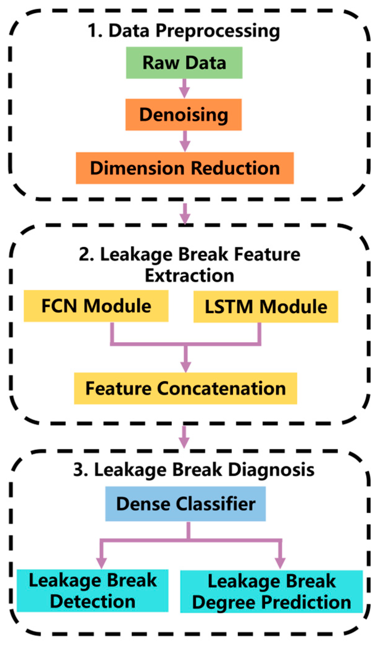
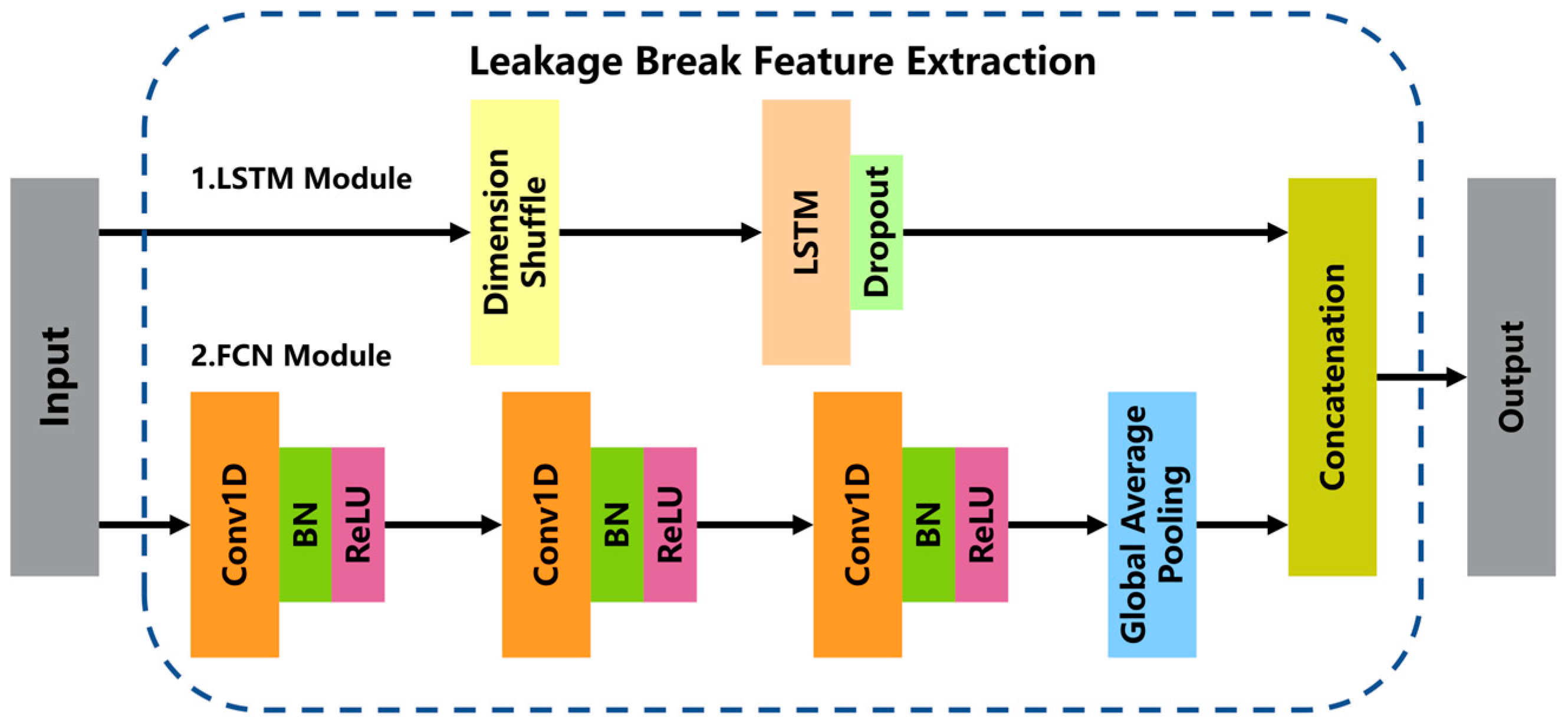
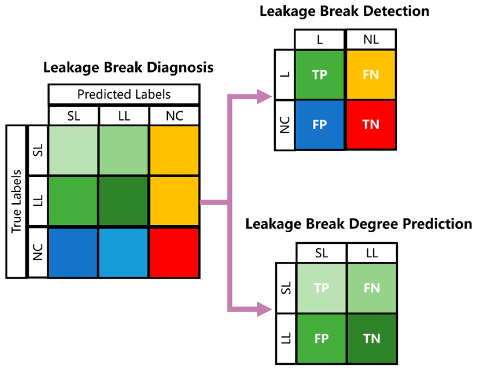
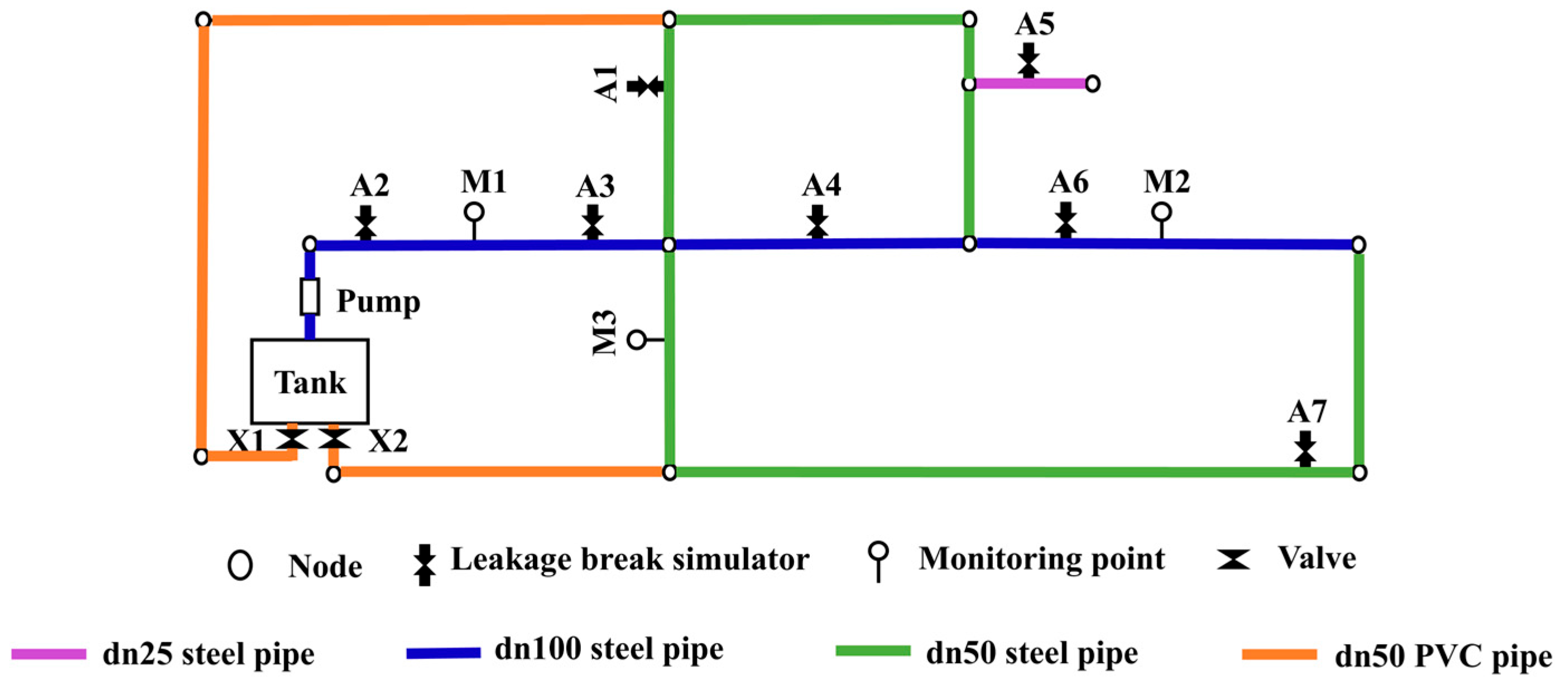
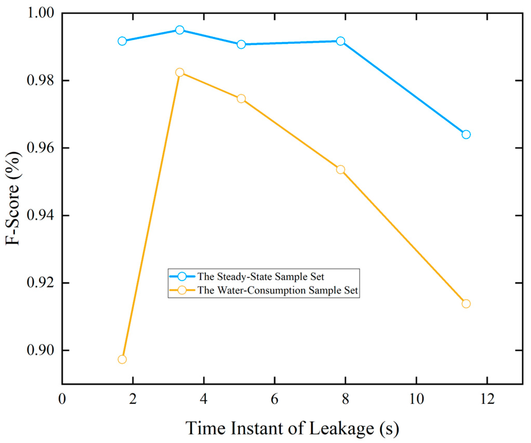
Building upon previous research and addressing the limitations of manual feature selection’s subjectivity and adaptability constraints, this study aimed at developing a novel leakage break diagnosis method for WDNs. Given the features extracted by an RNN and CNN based on their respective principles are different, and the features extracted by them are complementary in some time-series data classification tasks, this paper proposes a concatenating deep neural network, specifically an LSTM-FCN model, to complete the classification task of time-series data. First, the original high-frequency pressure data is preprocessed through filtering and frequency reduction. Second, the LSTM module and FCN module are used to learn the time information and local information in the data, respectively, and complete the extraction of leakage break features. Finally, the extracted leakage break features are sent to a classifier to output the predicted label, which includes the diagnosis information of leakage break detection and leakage break degree prediction. An experimental network is established to simulate leakage break events and leakage break-free events. A steady-state sample set and a variable water-consumption sample set were obtained to verify the performance of the proposed method. Meanwhile, the influence of several factors on the method performance is also discussed, such as the sample length and leakage break time instant. The experimental results validate the methodology’s reliability and diagnostic accuracy in the test WDN environment, where the LSTM-FCN model exhibited consistent performances across diverse operational conditions.

Based on the above analysis, the motivation of this study was to overcome the limitations of manual feature extraction methods, which often suffer from subjectivity and poor adaptability, by developing an automated and robust leakage break diagnosis approach for WDNs.

Traditional methods for detecting water losses in WDNs often involve techniques such as the division into District Metered Areas (DMAs), flow balancing, loss indicator determination, and the analysis of minimum night flow (MNF). These methods provide valuable insights into system efficiency and help identify potential leakage breaks. The DMA method divides the network into manageable sections for more precise monitoring, while flow balancing compares inflows and outflows to assess losses. The MNF analysis method, based on the observation of water usage during off-peak hours, helps detect anomalies indicative of leaks. However, these conventional techniques face limitations in addressing the complexity and dynamic nature of WDNs, especially under varying operational conditions and water-consumption patterns. In contrast, the proposed LSTM-FCN-based method in this study leverages high-frequency pressure data to provide a more adaptive and accurate approach to leakage break diagnosis, addressing these challenges with improved reliability and predictive power.

Therefore, the objective of this work was to propose a novel deep learning-based method that leverages high-frequency pressure data to detect and classify leakage break events with a high reliability and accuracy. Specifically, a concatenated deep neural network architecture, the LSTM-FCN model, was designed to exploit the complementary strengths of RNNs and CNNs in time-series feature extraction.

In this paper, we refer to the detection of newly occurred leakage events as “leak break” detection, rather than traditional “leak detection.” The term “leak detection” may refer to long-term background leakage. And compared with sudden burst events, the leakage flow in this research was relatively low. In many previous studies, particularly those using transient test-based methods, the focus was on identifying pre-existing leaks that persisted over time. These conventional techniques, such as inverse transient analysis (ITA), analyze the reflection of pressure waves caused by long-term leakages under controlled conditions. To avoid confusion, we clarify that our focus was on identifying pressure transients caused by newly generated leaks in a water distribution network.

To clarify the scope of this study, we emphasize that our goal was not to locate pre-existing leaks, but to detect the emergence of new leakage break events in real-time by analyzing pressure transients caused by their sudden appearance.

Transient wave-based methods are widely used for leak detection because they capture high-frequency pressure variations caused by structural disturbances. Among them, inverse transient analysis (ITA) is a common and effective diagnostic technique.

Capponi et al. proposed the Network Admittance Matrix Method (NAMM), which formulates water hammer equations in the frequency domain and uses a Laplacian matrix for leak detection. Validated on a branched system, it showed accurate leak localization under varying conditions [22]. Wang and Ghidaoui introduced a linearized transient model with maximum likelihood estimation to detect multiple leaks, demonstrating a high accuracy in viscoelastic pipes [23]. Tong-Chuan et al. reviewed five types of transient wave-based methods, highlighting their strengths but noting their reliance on the prior knowledge of pipeline topology and complex signal processing, which may limit adaptability in unknown systems [24]. A wider range of studies have demonstrated the potential of pressure transient tests in locating such persistent leaks. Classical methods using pressure wave analysis and physical modeling have been validated in labs and field tests. Studies like those cited by Brunone et al. examined how the leak location, pipe material, and boundary conditions affect the transient responses [25].

While these approaches are effective for detecting passive leak signals in controlled settings, they rely heavily on detailed system models and repeated transient tests. This limits their use in large or poorly documented networks, where rapid deployment is needed.

Unlike conventional transient-wave-based methods, our approach does not rely on previous knowledge of the pipe network’s topology. Instead, we applied a data-driven method that learns from high-frequency pressure signals to distinguish normal consumption from anomalies caused by leakage breaks.

Furthermore, most of these methods are mainly used for regular checks or planned tests on old pipelines, not for the quick detection of new leak breaks as soon as they happen. In contrast, our study focused on the detection of newly occurred leak breaks, which generate transient signals different from those of long-term leaks. By adopting a data-driven deep learning method, we can quickly identify leak-induced transient patterns from normal water consumptions directly from the data, making it suitable for real-time applications in complex, dynamic distribution systems.

The novelties of this study are threefold: (1) the application of the LSTM-FCN model to automatically learn both temporal and local features from high-frequency pressure data for leakage break diagnosis; (2) the establishment of an experimental water distribution network to generate steady-state and variable consumption sample sets, providing a comprehensive evaluation of the method under realistic conditions; and (3) a detailed investigation of the impact of the sample length and leakage break occurrence timing on the diagnostic performance, offering practical insights for future field applications.

Although background leakage is commonly present in water distribution networks, the detection of sudden leakage breaks remains valuable for operation and maintenance, it still holds practical value in specific scenarios—such as industrial cooling systems or sensor-equipped pipeline sectors—where operational anomalies must be promptly analyzed. In such cases, high-frequency pressure monitoring is feasible and meaningful. Therefore, this study did not aim to propose a universal solution, but rather a targeted framework for systems where leak break detection remains relevant.

2. Methods

The leakage break diagnosis method proposed in this paper consists of three parts, which are data preprocessing, leakage break feature extraction, and leakage break diagnosis, as illustrated in Figure 1.

This framework was designed as a diagnostic approach for specific monitoring scenarios—such as DMA sectors equipped with high-frequency pressure sensors—rather than as a universal solution for all urban WDNs. In such settings, the accumulation of monitoring and experimental data enables the early detection of newly occurring leakage breaks, which can support an emergency response and maintenance planning.

2.1. Data Preprocessing

2.1.1. Data Denoising

The raw data collected by high-frequency pressure sensors inevitably contain noise that obscures leakage break signals. We applied a Butterworth band-stop filter to remove the noise in a specific frequency range and enhance the signal quality.

The filter works in the frequency domain, isolating noise components via Fourier transform. The Fourier transform is used here to decompose the original time-domain signal into its frequency components, allowing us to isolate and remove specific frequency bands associated with noise. This enables effective noise elimination by intercepting the signal of a certain frequency. Its formulation is shown in Equations (1) and (2):

$$H\left(f\right)={\displaystyle \frac{1}{\sqrt{1+{(f/f_c)}^{2n}}}}, 0\le f<\mathsf{\pi }$$

(1)

$$H\left(f\right)={\displaystyle \frac{1}{\sqrt{1+{((2\mathsf{\pi }-f)/(2\mathsf{\pi }-f_c))}^{ 2n}}}}, \mathsf{\pi }\le f<2\mathsf{\pi }$$

(2)

where n is the order of the function, f is the frequency, and f_c is the cut-off frequency.

This process enhances the visibility of key features, such as the negative pressure wave and pressure drop, facilitating more effective feature extraction.

2.1.2. Data Dimension Reduction

High sampling rates can introduce redundancy and increase the computational load. To address this, we apply an average pooling layer to downsample the data, as shown in Equation (3):

$$D_i^{\prime }={\displaystyle \frac{{\sum }_{t=1}^k{D}_{\left(i-1\right)s+t}}{k}}$$

(3)

where D and $D^{\prime }$ are the samples before and after the dimension reduction, k is the kernel size, and s is the stride.

This step reduces the data size while retaining critical temporal features for leakage break analysis.

2.2. Leakage Break Feature Extraction

As shown in Figure 2, the prepossessed data is fed into the LSTM module and the FCN module in parallel to extract different leakage break features. The deep learning models were implemented using the TensorFlow library (Python 3.8, TensorFlow). After that, the two leakage break features are concatenated in series to obtain the output vector, which is sent to the leakage break diagnosis module in the next part.

2.2.1. LSTM Module

The LSTM module includes a dimension shuffle layer and an LSTM layer. The dimension reconstruction of input data is completed in the dimension shuffle layer to improve the performance and efficiency of the LSTM layer [26]. As a variant of an RNN, the LSTM layer sets the forget gate, input gate, and output gate based on gating functions so as to have the mechanisms of memory and forgetting and solve the vanishing gradient problem in the RNN [14]. At time step t, a series of equations are calculated in turn to update the parameter values [27].

The dropout layer is connected behind the LSTM layer, which is used to make neurons stop working with a certain probability during the forward propagation process so as to prevent overfitting and obtain a robust performance [18,27].

2.2.2. FCN Module

The structure of the FCN module is shown in Figure 2. The Conv1D layer, which uses the trainable convolution kernel to perform multiplication and addition operations with the input time-series data, can extract local features at different positions. For each Conv1D layer, there is a batch normalization (BN) layer and a ReLU activation layer connected to it to avoid gradient disappearance and gradient explosion in the learning process [28,29].

The leakage break feature obtained after three convolutions is compressed through the global average pooling layer to reduce the number of parameters and the risk of overfitting [23]. Compared with average pooling, global average pooling takes the average of the data in the whole feature map instead of the time window, which means the output is the mean of the whole input vector.

2.2.3. Output Module

The features extracted from both the LSTM and FCN modules are represented as vectors. In the feature concatenation layer, these two feature vectors are concatenated along the feature dimension to form the final leakage break feature representation. This concatenated feature vector is then passed through a fully connected layer, where nonlinear transformations are applied to map the features into the output space for sample classification.

In the output layer, each neuron corresponds to a specific class. For a given sample, the predicted class label is determined by the neuron with the highest output probability. Thus, the LSTM-FCN model outputs the class that best matches the leakage break characteristics of the input sample.

To ensure the robustness and generalizability of the model, subsequent sections detail the evaluation metrics used to assess model performance, as well as the procedures for parameter calibration and experimental setup.

This fusion is expected to enhance the model’s ability to capture dynamic patterns and localized anomalies associated with leakage break events. To further validate the effectiveness of this combined architecture, comparative experiments with stand-alone LSTM, FCN, and ANN models were conducted later. These comparisons demonstrated that the integration of temporal and spatial feature extractors contributed significantly to the improved leakage break classification performance.

2.3. Leakage Break Diagnosis

For leakage break diagnosis in actual WDNs, water companies expect to detect leakage break events and know about the leakage break severity, which can help them launch the corresponding level of leakage break response. However, it should be noted that pressure changes are not only caused by leaks but also by daily operations and random water usage, which may affect the diagnosis accuracy. The following series of operations can be performed to obtain the predicted label.

The final leakage break features are fed to the dense classifier as the input vector. The input vectors are passed through a fully connected layer for nonlinear transformation and then mapped to the output space to complete the classification of the samples. And here is a matrix operation on the input vector. The trainable weight matrix, the trainable bias vector, and the softmax activation function are used to introduce non-linearity [27]. The outputs of the dense classifier and the softmax activation function are shown in Equation (4) and Equation (5), respectively:

$$output=\alpha (\omega x+b)$$

(4)

$$\alpha (x_i)={\displaystyle \frac{e^{x_i}}{{\sum }_i{e}^{x_i}}}$$

(5)

where α is the activation function, ω is the trainable weight matrix, b is the trainable bias vector, x_i is the output value of the ith node (there are many output nodes in the fully connected layer), and α(x_i) is the output probability distribution of the ith node.

The leakage break diagnosis is described as a three-classification task in this paper: normal condition (NC), small leakage break (SL), and large leakage break (LL). The leakage break amount of NC is 0. In practice, although background leakage may still exist in water distribution networks, NC here refers to the absence of sudden leakage break events. The distinction between SL and LL is based on whether the leakage break exceeds 1 L/s (if it exceeds, it is classified as LL; otherwise, it is classified as SL). In practical cases, it is essential to distinguish between normal operating conditions and leakage break events. Therefore, the first goal of the classification task is to enable the model to identify whether a leak break has occurred, which suits real-world leak break detection needs in urban WDNs. This ensures that the model captures the fundamental difference between regular operation and abnormal events. A three-class framework also helps the model learn more specific differences in transient pressure patterns. By further distinguishing SL and LL, the model is encouraged to extract more detailed features, which are often overlooked in binary classification tasks. Compared with binary classification, this approach adds useful complexity, which can reduce the risk of overfitting during training and improve the model’s generalization ability. It also allows a more thorough evaluation of how well the model can detect both large and small leak breaks in the system. From a practical perspective, distinguishing between small and large leak breaks can provide water utilities with useful information for decision-making. For instance, larger leak breaks may require prioritized intervention to prevent serious water loss. This classification approach aligns better with practical utility needs. Therefore, even though the leak size thresholds are set manually, they are based on real-world leak management needs. It is acceptable to set more classes according to different needs [30]. The number of categories can be set according to your needs.

The performance of the leakage break diagnosis was evaluated from two aspects in this study: leakage break detection and leakage break degree prediction. The three-class classification results based on the proposed method are represented as an initial 3 × 3 confusion matrix of leakage break diagnosis, as shown in Figure 3. When the performance of leakage break detection is evaluated, the SL class and the LL class can be combined as the L class, so as to obtain the 2 × 2 confusion matrix of leakage break detection. When it comes to leakage break degree prediction, the NC class is removed to obtain the 2 × 2 confusion matrix of leakage break degree prediction. In this study, the diagnosis of leakage break detection and leakage break degree prediction are performed simultaneously, making the leakage break detection task a three-class classification problem.

In Figure 3, the colors are used to visually distinguish prediction results: the L class predicted as L is shown in green shades, with different shades indicating SL and LL subclasses; NL predicted as L is represented in orange shades, also with depth variations for SL and LL subclasses; L predicted as NC is shown in blue shades, differentiated by SL and LL depths; and NL predicted as NC is indicated in red. This color coding helps to clearly differentiate prediction outcomes and subclasses within the confusion matrix.

By removing the need for detailed hydraulic models or network maps, the proposed method reduces the setup complexity and facilitates adaptation to different WDNs. This contributes to the practicality of real-time monitoring, especially in situations where hydraulic models or detailed system maps are unavailable.

3. Experiments

3.1. Experimental Procedure

3.1.1. Experimental Setup

In this study, an experimental network was built to simulate leakage break events, whose topological structure is shown in Figure 4. The total length of the experimental network was 52 m, which included a tank, a water pump (Model: CDE360, Shenzhen Kangyuan Electric Technology Co., Ltd., Shenzhen, China), 3 pipes with a 100 mm diameter, 11 pipes with a 50 mm diameter, and 1 pipe with a 25 mm diameter. Three high-frequency monitoring points were set. All monitoring points were considered equivalent for this purpose. Each consisted of a high-frequency pressure sensor (Model: MPM4961T4, Huizhong Instrumentation Co., Ltd., Tangshan, China) with a sampling frequency of 10,000 Hz and an ultrasonic flow meter (Model: SCL-61D5, Huizhong Instrumentation Co., Ltd., Tangshan, China) with a sampling frequency of 1 Hz. High-frequency pressure sensors were used to collect the pressure fluctuation signal before and after the leakage break events occurred, and flow meters were used to estimate the leakage break flow of leakage break events. Meanwhile, seven leakage break simulators were set to simulate leakage break events. Each consisted of a leakage break hole, a ball valve, and plastic pipes. The leakage break hole’s diameter of the leakage break simulator A6 was 32 mm, while it was 15 mm for the others.

Leakage break simulators can be used to simulate leakage break events and variations in water consumption in actual networks. Leakage break events are simulated by rotating the ball valve to a certain angle in an instant, and variations in water consumption can be simulated by rotating the ball valve slowly and randomly.

Different working conditions can be set by adjusting the operating parameters of the water pump and the opening degree of valves X1 and X2. The total flow rate in the pipeline was adjusted by regulating the opening degree of two valves in the experimental setup, which allowed for the simulation of various water usage conditions during both day and night. The initial pressure of the network was in the range of 5–30 m, and the total flow of the network was in the range of 2.5–23 L/s.

3.1.2. Experimental Data Collection

In the actual network, variations in user water consumption will affect the performance of a leakage break diagnosis. Hence, a steady-state sample set and a water-consumption sample set were established in this study so as to explore the adaptability of the leakage break diagnosis model. The simulation of the steady-state water usage was implemented by rotating the ball valve to a certain angle before the experiment and maintaining it. And the simulation of the water-consumption sample set was implemented by rotating the ball valve slowly and randomly. During the simulation of the steady-state sample set, the valve opening was set to 45° and 90°; for the water-consumption sample set, the valve rotation range was 30° to 75°.

There were 1044 leakage break samples and 1044 leakage break-free samples in the steady-state sample set where there was no simulation of the variations in the water consumption. Meanwhile, there were 261 leakage break samples and 261 leakage break-free samples in the water-consumption sample set where the simulation of variations in the water consumption was added. The flow of leakage break events is in the range of 0.04–9.5 L/s.

The 1 L/s threshold used to distinguish small and large leak breaks was set to balance the sample distribution, which helped improve the model training and avoid bias toward one class. Since the machine learning needed to turn continuous leak sizes into categories, setting a threshold was necessary. This value is used as a starting point and can be adjusted in practice based on utility needs and model performance.

3.2. Performance Metrics and Model Parameters

3.2.1. Performance Metrics

For the confusion matrix of leakage break detection, the water company pays more attention to positive (the L class) compared with negative (the NC class). Hence, the F-Score was selected to evaluate the performance of leakage break detection, which is calculated by Formulas (6)–(8):

$$P={\displaystyle \frac{{TP}_n}{{TP}_n+{FP}_n}}$$

(6)

$$R={\displaystyle \frac{{TP}_n}{{TP}_n+{FN}_n}}$$

(7)

$$F={\displaystyle \frac{\left(1+{\beta }^2\right)\times P\times R}{\left({\beta }^2\times P\right)+R}}$$

(8)

where TP_n, FP_n, and FN_n represent the numbers of TP, FP, and FN; P, the Precision, reflects the classification reliability of the leakage break events; and R, Recall, reflects the detection capability. The Precision and Recall are often negatively correlated, and F, the F-Score, is the harmonic average of them to reflect the synthetic performance. β in Equation (8) is used to adjust the weights of P and R. β takes a value over 1 when the Recall is more important than the Precision in the task. Considering that the water company hopes to detect more leakage break events and can withstand certain false alarm events, β was taken as 2 in this study. These metrics were selected as they comprehensively reflected the model’s classification performance from multiple perspectives, which ensured a robust evaluation of the leakage break diagnosis effectiveness.

For the confusion matrix of leakage break degree prediction, positive (the SL class) and negative (the LL class) were on an equal footing, so the accuracy was selected to evaluate the performance of the leakage break degree prediction, whose formula is as follows:

$$A={\displaystyle \frac{{TP}_n+{TN}_n}{{TP}_n+{TN}_n+{FP}_n+{FN}_n}}$$

(9)

where A represents the accuracy, and TP_n, TN_n, FP_n, and FN_n represent the numbers of TP, TN, FP, and FN.

3.2.2. Model Parameters

Several values of f_c were taken in Equations (1) and (2) to compare the performances of data denoising. When f_c took a large value of 1 or 0.1, the sample was not completely filtered. When f_c took 0.001 or 0.0001, although the noise was basically eliminated, the useful information leakage break was almost completely removed. When f_c was taken as 0.01, the noise was eliminated to the greatest extent, and the useful information of the negative pressure wave and pressure drop caused by leakage break events was retained. Therefore, f_c was taken as 0.01 in this study. k and s in Equation (3) were both taken as 100 since the sampling frequency was 10,000 Hz.

The hyperparameter settings were selected based on previous studies [26] and adjusted to fit the characteristics of the high-frequency pressure data in this study, balancing the model’s learning capability and computational efficiency. In the LSTM module, the number of neurons of the LSTM layer was taken as 128 to adapt to the dataset, and the probability of the dropout layer was taken as 80%. In the LSTM module, the numbers of filters of the three Conv1D modules were 128, 256, and 128. The kernel sizes of the three Conv1D modules were 8, 5, and 3. Considering the flow distribution of the leakage break samples in the two sample sets, 1 L/s was used as the dividing line of leakage break flow to divide the leakage break events into large and small leakage break events.

3.3. Discussion

3.3.1. Influence of Sample Length

The change in sample length means the difference in the quantity of information contained in the samples, which had a significant impact on the performance of the LSTM-FCN deep learning model. Nine length gradients from 2 s to 18 s were set in this study to explore the influence of the sample length. The ratio of the training set to the testing set was 7:3.

It can be seen from Figure 5a that with the increase in the sample length, the F-Score of the leakage break detection of the LSTM-FCN deep learning model increased first and then decreased. In the steady-state sample set, the F-Score increased from 98.57% at 2 s to 99.64% at 12 s and then decreased with the continuous increase in the sample length. In the water-consumption sample set, the F-Score increased from 92.11% at 2 s to 95.31% at 12 s and then decreased to 94.48% at 18 s. Therefore, it shows that the model could continue to learn more leakage break information with a short sample length. However, when the sample length increased to a certain level, the further increase no longer improved the model performance, but caused a redundancy of information and an increase in the model computation. In addition, the change in sample length from 2 s to 8 s had a particularly obvious impact on the model performance in the water-consumption sample set. This was because there were huge pressure fluctuations in the network environment with variations in the water consumption, and the shape of the pressure drop caused by the leakage break and variations was similar in a short length, which disturbed the diagnosis of the model. When the sample length increased, there was enough information to judge whether it was the pressure drop that caused the decrease in the average pressure level and then successfully diagnose the leakage break events and avoid false alarms.

Figure 5b shows the leakage break degree prediction performance of the LSTM-FCN deep learning model on two sample sets. The influence of the sample length on the leakage break degree prediction performance was similar to that on the leakage break detection. And the results prove that the LSTM-FCN deep learning model could effectively extract the information about the leakage break degree, which was beneficial to the decision-making for the leakage break repair response level of the water company.

The results in Figure 5b show that the accuracy in the steady-state sample set was 10% lower than that in the water-consumption sample set, and this can be explained by

Table 1. The percentage of leakage break samples within a certain leakage break flow range in the two sample sets.

Leakage Break Flow Range	The Steady-State Sample Set	The Water-Consumption Sample Set
0.9–1.1 L/s	12.42%	2.60%
0.8–1.2 L/s	20.70%	10.39%

. The percentage of leakage break samples whose leakage break flow was in the range of 0.9–1.1 L/s or 0.8–1.2 L/s in the steady-state sample set was higher than that in the water-consumption sample set. These leakage break samples were hard to correctly classify because their leakage break flow was close to 1 L/s, which means there was similar leakage break information to the leakage break flow.

Therefore, the optimal sample length was 12 s, where the LSTM-FCN deep learning model achieved the best performance in the leakage break detection and leakage break degree prediction on both sample sets. Hence, the sample length was taken as 12 s in the following experiments of this study.

3.3.2. Influence of Leakage Break Time Instant

For the leakage break diagnosis in actual WDNs, the time instant of a leakage break event in the time-series sample was completely random, which means each time instant had the same possibility of a leakage break. Therefore, it was necessary to explore the influence of different time instants on the leakage break diagnosis performance and improve the applicability of the leakage break diagnosis model in actual WDNs.

In Section 3.3.1, 12 s was determined as the optimal sample length, and the leakage break events all occurred in the middle of the sample (at 6 s) by default. Therefore, 13 evenly distributed time instants were selected as time instants where leakage break events may occur in this section. The original sample sets were translated to obtain 13 groups of similar sample sets. And the only difference between them was that the leakage break occurred at different time instants.

The LSTM-FCN deep learning model with the best performance in Section 3.3.1 was applied to the testing sets of sample sets with 13 time instants of leakage breaks, as shown in Figure 6. The LSTM-FCN deep learning model achieved the best performance in both sample sets with the time instant of the leakage break at 6 s. However, the performance of the model decreased significantly in the sample sets with other time instants of leakage breaks. Therefore, it can be inferred that when the training set contained samples with only one time instant of a leakage break, it was hard for the model to diagnose the leakage break events and obtain information about the leakage break that occurred at other time instants in the sample. In the actual WDNs, leakage break events always occurred suddenly, so it was hard to know the time instant. In order to enhance the adaptability of the LSTM-FCN deep learning model, it was necessary to make the time instant of leakage break cover the whole sample length in the training set. In addition, for the steady-state sample set, the closer the time instant of a leakage break was to 6 s, the better the performance of the model was. For the water-consumption sample set, even though the interference of variations affected the model’s ability to obtain leakage break information, 6 s remained the best.

Considering the influence of the time instant of the leakage break on the model performance, the training set needed to be expanded to obtain more information about the time instant of the leakage break. Finally, 25 sample sets, where the interval of the adjacent leakage break time instants was 0.5 s, were combined into one sample set as the training set to cover the entire sample length. At the same time, five time instants of the leakage break were randomly generated to form the testing set. The five time instants were 1.7026 s, 3.3232 s, 5.0612 s, 7.8658 s, and 11.408 s. The leakage break detection performance of the LSTM-FCN deep learning model on the five testing sets are shown in Figure 7. With the improvement in the training set, the LSTM-FCN deep learning model showed better adaptability to the randomness of the leakage break time instant and obtained F-Scores of more than 89% on both the steady-state sample set and water-consumption sample set.

3.3.3. Performance on Leak Break Level Classification Under Different Sampling Conditions

To further verify the model’s ability to identify different leakage break levels, we evaluated its performance on a binary classification task distinguishing small leak breaks from large leak breaks in two different datasets: the steady-state sample set and the water-consumption sample set. The confusion matrices for both conditions are shown in Figure 8. And the accuracy of the small and large leak breaks in the two sample sets are shown in

Table 2. The accuracy of the small and large leak breaks in the two sample sets.

Leak Break Level	The Steady-State Sample Set	The Water-Consumption Sample Set
Small leak breaks	76.2%	89.4%
Large leak breaks	81.3%	96.6%

.

In the steady-state condition (Figure 8a), the model correctly identified the following:

A total of 141 out of 185 small leak break cases, which yielded an accuracy of 76.2%.

A total of 126 out of 155 large leak break cases, which yielded an accuracy of 81.3%.

These results demonstrate the model’s reliable ability to differentiate between minor and major leak breaks, even when transient events were absent. The relatively high accuracy in both classes indicates that the pressure patterns under steady conditions still carried distinguishable features related to the leak break size, which could be effectively captured by the model.

In the water-consumption sample set (Figure 8b), the model performed even more accurately:

A total of 42 out of 47 small leak break cases were correctly classified, with an accuracy of 89.4%.

A total of 28 out of 29 large leak break cases were correctly classified, with an accuracy of 96.6%.

This result shows a clear improvement compared with the steady-state pattern. The presence of dynamic pressure changes appeared to enhance the signal difference between the small and large leak breaks, which made them more distinguishable for the model. Such a performance highlights the potential of transient-based data collection strategies in improving the leak diagnosis effectiveness in practical applications.

3.4. Validation of Leakage Break Diagnosis Performance

In order to verify the applicability of the leakage break diagnosis method proposed in this paper, new leakage break samples and leakage break-free samples were used to test the LSTM-FCN deep learning model. The testing set contained 34 leakage break events and 68 leakage break-free events in the steady-state sample set, while 10 and 20 were used in the water-consumption one. Ten new time instants of leakage break were randomly generated to expand the testing set and simulate the randomness of the leakage break events in the WDNs. In the 52 m experimental network, three high-frequency pressure sensors were deployed. The analysis showed that the samples collected by the three monitoring points were equivalent in terms of the leakage break feature representation, and the detection and classification performance remained stable regardless of which sensor data was used. This indicates that 1–3 monitoring points were sufficient for effective leakage break detection and size classification in a pipe network of this length, given the relatively dense sensor deployment.

In addition, the LSTM model, the FCN model, and the ANN model based on feature extraction were also applied to serve as baseline models, which helped demonstrate the superiority of the proposed LSTM-FCN model. All the models were tested on a new set of experimental data to ensure a fair comparison. This comparison not only verified the effectiveness of the LSTM-FCN architecture but also highlighted the performance improvement brought by the integration of temporal and spatial feature extraction for leakage break diagnosis. Statistical features, which contained mean, standard deviation, skewness, and kurtosis, and wavelet features, which contained the detail coefficients of levels three, four, and five for the Haar wavelet, were extracted to train and test the ANN model [30].

The validation of the proposed LSTM-FCN-based leakage break diagnosis method was carried out using specific performance metrics in this study. Figure 8 presents the F-Score results to evaluate the model’s balance between the Precision and Recall, highlighting the effectiveness of the leakage break event classification. Figure 9 shows the accuracy comparisons between the different models, demonstrating the superior performance and generalization ability of the LSTM-FCN model across varying operational conditions. These metrics comprehensively validated the reliability and robustness of the proposed methodology.

The leakage break detection performances of the four models on the new testing set are shown in Figure 9. In the steady-state sample set, the LSTM-FCN deep learning model obtained an F-Score that was over 4% better than the LSTM model and the FCN model, which indicates that the combination of the two models increased the leakage break information and improved the leakage break diagnosis performance. In addition, the LSTM-FCN deep learning model also performed better than the ANN model. The result illustrates that the leakage break features self-extracted with the LSTM-FCN deep learning model included more leakage break information than the artificially selected leakage break features. In the water-consumption sample set, the F-Score of the four models inevitably decreased due to the interference of variations in the water consumption. The LSTM-FCN deep learning model obtained the best F-Score of 81.76% among the four models and showed the best adaptability to severe background pressure fluctuations in the actual WDN.

The performance of the leakage break degree prediction of four models on the new testing set is shown in Figure 10, among which in the steady-state sample set was worse than that in the water-consumption sample set. And this was mainly caused by the difference in the distribution of the leakage break flow in two sample sets, which was analyzed in Section 3.3.1. The LSTM-FCN deep learning model had the best comprehensive performance on the two sample sets and reached an average accuracy of 85%, which showed its ability to obtain information about the leakage break degree. Although the FCN model performed well on the steady-state sample set, it showed a poor performance on the water-consumption sample set. On the other hand, the FCN model performed well on the water-consumption sample set but exhibited a poor performance on the steady-state sample set and deteriorated in the leakage break detection under water-consumption conditions. Overall, the LSTM-FCN model demonstrated good performances on both types of sample sets.

The results on the testing sets from the new leakage break events and leakage break-free events illustrated that the proposed leakage break diagnosis method based on the LSTM-FCN deep learning model could effectively learn the leakage break features in high-frequency time-series data and had a high accuracy on the leakage break detection and leakage break degree prediction of new samples in the WDNs. Compared with previous studies using FCN [20] and LSTM [21], which relied on conventional classification models, the proposed LSTM-FCN method showed a better diagnostic accuracy and robustness across different operational conditions. This improvement can be attributed to the model’s ability to automatically extract temporal and spatial features from high-frequency pressure data. Meanwhile, the proposed method also had good adaptability to the variations in water consumption in the actual WDNs. Although the proposed method could not directly identify the precise location of a leak break, it served as a fast and effective warning mechanism to indicate the presence and severity of leak events. Such early detection can support subsequent response actions, such as deploying leak localization algorithms or on-site inspections.

4. Conclusions

A leakage break diagnosis method based on the LSTM-FCN neural network model from high-frequency pressure data is proposed in this paper. First, data preprocessing is used to avoid the influence of noise and information redundancy. Second, the LSTM module and the FCN module are used to extract and combine different leakage break features. Finally, the leakage break feature is sent to a dense classifier to obtain the predicted result. The following conclusions were drawn:

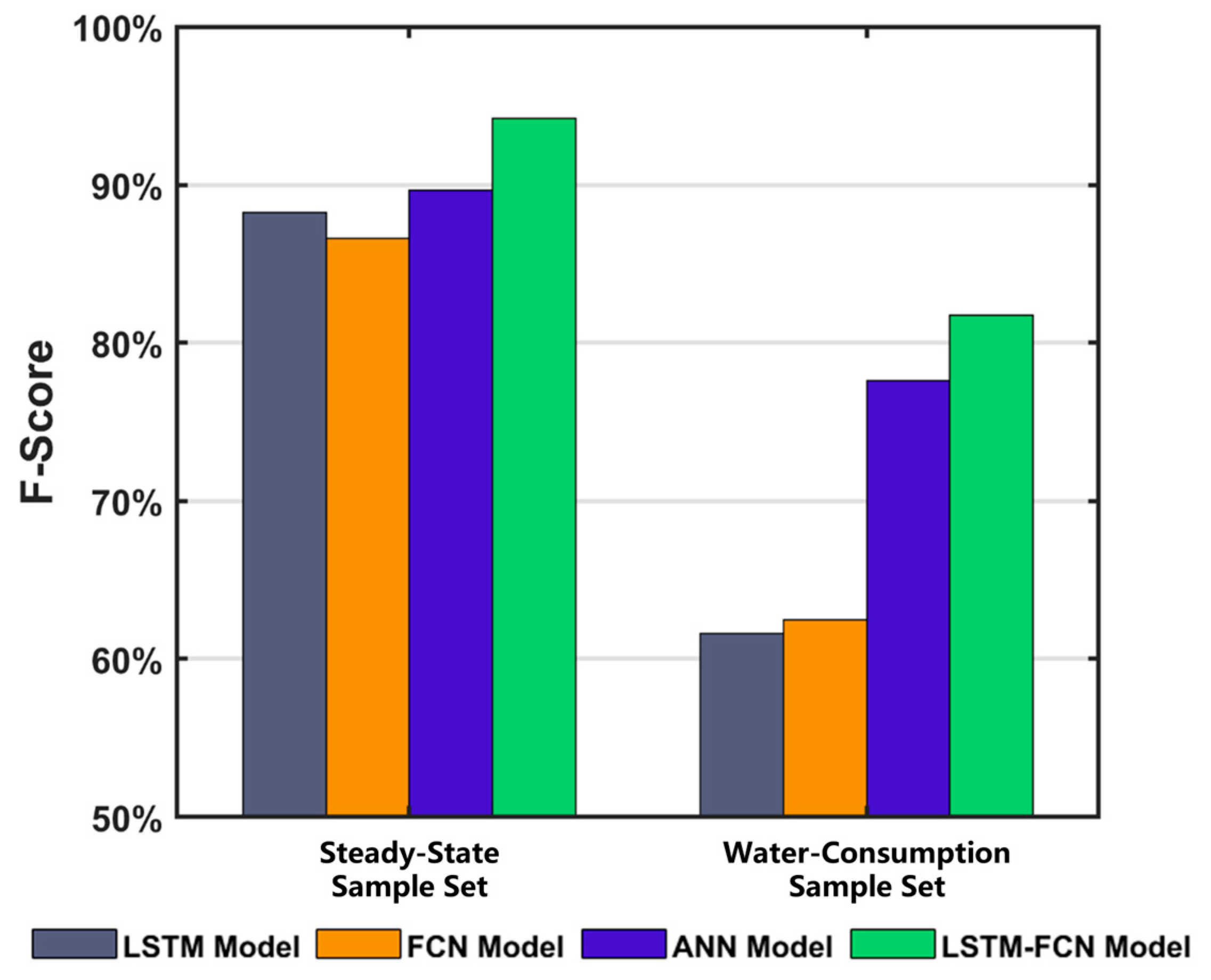
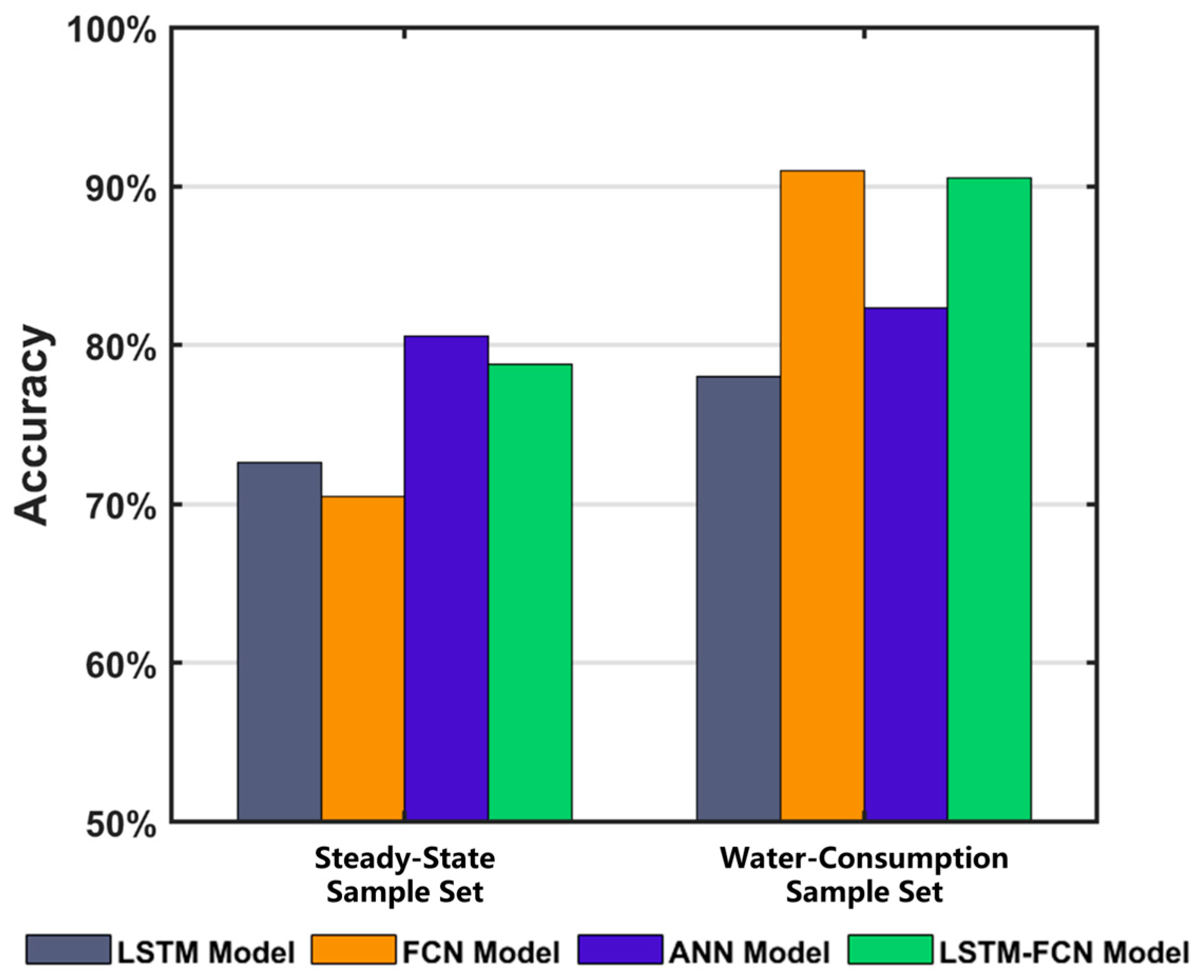
The LSTM-FCN deep learning model was well qualified for the three-classification task of leakage break diagnosis and had a high accuracy in the leakage break detection and leakage break degree prediction on the high-frequency pressure data. The LSTM model and FCN model could extract different leakage break features. And the LSTM-FCN deep learning model obtained a better performance of leakage break diagnosis because of the combination of the two different leakage break features. The trained LSTM-FCN deep learning model showed a good performance on both the steady-state sample set and water-consumption sample set, which illustrated that the model could be highly robust to the variations in water consumption in the actual WDNs.

To ensure the effectiveness of the proposed LSTM-FCN-based leakage break diagnosis method, certain conditions must be met. The approach requires high-frequency pressure data with sufficient temporal resolution to capture transient features related to leakage break events. The pipeline system should have a relatively stable hydraulic background, as excessive environmental noise or frequent operational fluctuations may mask the leakage break-induced patterns. Additionally, accurate sensor calibration and stable sensor placement are essential for reliable data acquisition. The method may be less effective in systems with sparse sensor coverage, a low sampling frequency, or highly irregular pressure variations caused by external disturbances.

This study confirmed the feasibility of using an LSTM-FCN model for classifying leakage break severity levels in a laboratory-based water distribution system. The experimental results demonstrate that the model was sensitive to different leakage break conditions, which supports its potential as a diagnostic tool in more complex leakage break scenarios. Although a leakage break always exists in real systems, the “normal condition” in our setup was used as a baseline to enhance model sensitivity to newly emerging leakage breaks. The ability to differentiate the leakage break severity can assist utilities in better management and also forms the basis for further tasks, including leakage break quantification and spatial localization. Future research will focus on reducing the reliance on labeled data by exploring semi-supervised and transfer learning techniques. Future work may also incorporate leak localization modules following the detection stage, enabling the system to not only identify the occurrence of a leak but also estimate its position. Combining classification-based detection with inverse transient analysis or data-driven localization algorithms could enhance the practical value of the proposed framework in real-world WDNs.

Although the experiments were conducted under laboratory conditions using pipes in a controlled environment, the proposed leakage break diagnosis method can be adapted for real-world WDNs. What is more, the model was also tested on unlabeled data under variable consumption patterns, indicating its capacity to generalize across unseen usage conditions. However, practical application in underground pipelines may face challenges, such as environmental noise and pressure fluctuations. Further field validation on real-world WDNs is needed to improve the model’s generalization ability. And the influence of the sensor number and spatial density on the leakage break localization accuracy will be further studied. The optimal deployment strategy for large-scale networks remains an open research question.

References

1. Boaz, L.; Kaijage, S.; Sinde, R. An overview of pipeline leak detection and location systems. In Proceedings of the 2nd Pan African International Conference on Science, Computing and Telecommunications (PACT 2014), Arusha, Tanzania, 14–18 July 2014; pp. 133–137. [Google Scholar]
2. Lang, X.; Li, P.; Zhang, B.; Cao, J.; Guo, Y.; Kan, Z.; Lu, S. Localization of multiple leaks in a fluid pipeline based on ultrasound velocity and improved GWO. Process Saf. Environ. Prot. 2020, 137, 1–7. [Google Scholar] [CrossRef]
3. Tijani, I.A.; Abdelmageed, S.; Fares, A.; Fan, K.H.; Hu, Z.Y.; Zayed, T. Improving the leak detection efficiency in water distribution networks using noise loggers. Sci. Total Environ. 2022, 821, 153530. [Google Scholar] [CrossRef] [PubMed]
4. Romano, M.; Kapelan, Z.; Savić, D.A. Evolutionary Algorithm and Expectation Maximization Strategies for Improved Detection of Pipe Bursts and Other Events in Water Distribution Systems. J. Water Resour. Plan. Manag. 2014, 140, 572–584. [Google Scholar] [CrossRef]
5. Zaman, D.; Tiwari, M.K.; Gupta, A.K.; Sen, D. A review of leakage detection strategies for pressurised pipeline in steady-state. Eng. Fail. Anal. 2020, 109, 104264. [Google Scholar] [CrossRef]
6. Rashid, S.; Qaisar, S.; Saeed, H.; Felemban, E. A Method for Distributed Pipeline Burst and Leakage Detection in Wireless Sensor Networks Using Transform Analysis. Int. J. Distrib. Sens. Netw. 2014, 10, 939657. [Google Scholar] [CrossRef]
7. Tian, X.; Jiao, W.; Liu, T.; Ren, L.; Song, B. Leakage detection of low-pressure gas distribution pipeline system based on linear fitting and extreme learning machine. Int. J. Press. Vessel. Pip. 2021, 194, 104553. [Google Scholar] [CrossRef]
8. Verma, A.; Zappalá, D.; Sheng, S.; Watson, S.J. Wind turbine gearbox fault prognosis using high-frequency SCADA data. J. Phys. Conf. Ser. 2022, 2265, 032067. [Google Scholar] [CrossRef]
9. Lay-Ekuakille, A.; Trotta, A.; Vendramin, G. FFT- based spectral response for smaller pipeline leak detection. In Proceedings of the 2009 IEEE Instrumentation and Measurement Technology Conference, Singapore, 5–7 May 2009; pp. 328–331. [Google Scholar]
10. Lay-Ekuakille, A.; Vendramin, G.; Trotta, A. Robust Spectral Leak Detection of Complex Pipelines Using Filter Diagonalization Method. IEEE Sens. J. 2009, 9, 1605–1614. [Google Scholar] [CrossRef]
11. Lay-Ekuakille, A.; Vendramin, G.; Trotta, A.; Vanderbemden, P. STFT-based spectral analysis of urban waterworks leakage detection. In Proceedings of the XIX IMEKO World Congress, Lisbon, Portugal, 6–11 September 2009; pp. 6–11. [Google Scholar]
12. Ferrante, M.; Brunone, B. Pipe system diagnosis and leak detection by unsteady-state tests. 2. Wavelet analysis. Adv. Water Resour. 2003, 26, 107–116. [Google Scholar] [CrossRef]
13. Srirangarajan, S.; Allen, M.; Preis, A.; Iqbal, M.; Lim, H.B.; Whittle, A.J. Wavelet-based Burst Event Detection and Localization in Water Distribution Systems. J. Signal Process. Syst. 2012, 72, 1–16. [Google Scholar] [CrossRef]
14. Lee, C.-W.; Yoo, D.-G. Development of Leakage Detection Model and Its Application for Water Distribution Networks Using RNN-LSTM. Sustainability 2021, 13, 9262. [Google Scholar] [CrossRef]
15. Kang, J.; Park, Y.J.; Lee, J.; Wang, S.H.; Eom, D.S. Novel Leakage Detection by Ensemble CNN-SVM and Graph-Based Localization in Water Distribution Systems. IEEE Trans. Ind. Electron. 2018, 65, 4279–4289. [Google Scholar] [CrossRef]
16. Xiao, R.; Hu, Q.; Li, J. Leak detection of gas pipelines using acoustic signals based on wavelet transform and Support Vector Machine. Measurement 2019, 146, 479–489. [Google Scholar] [CrossRef]
17. Aljameel, S.S.; Alomari, D.M.; Alismail, S.; Khawaher, F.; Alkhudhair, A.A.; Aljubran, F.; Alzannan, R.M. An Anomaly Detection Model for Oil and Gas Pipelines Using Machine Learning. Computation 2022, 10, 138. [Google Scholar] [CrossRef]
18. Zhao, L.; Mo, C.; Ma, J.; Chen, Z.; Yao, C. LSTM-MFCN: A time series classifier based on multi-scale spatial–temporal features. Comput. Commun. 2022, 182, 52–59. [Google Scholar] [CrossRef]
19. Han, Y.; Zhang, S.; Geng, Z. Multi-Frequency Decomposition with Fully Convolutional Neural Network for Time Series Classification. In Proceedings of the 2018 24th International Conference on Pattern Recognition (ICPR), Beijing, China, 20–24 August 2018; pp. 284–289. [Google Scholar]
20. Wang, Z.; Yan, W.; Oates, T. Time series classification from scratch with deep neural networks: A strong baseline. In Proceedings of the 2017 International Joint Conference on Neural Networks (IJCNN), Anchorage, AK, USA, 14–19 May 2017; pp. 1578–1585. [Google Scholar]
21. Zuo, Z.; Ma, L.; Liang, S.; Liang, J.; Zhang, H.; Liu, T. A semi-supervised leakage detection method driven by multivariate time series for natural gas gathering pipeline. Process Saf. Environ. Prot. 2022, 164, 468–478. [Google Scholar] [CrossRef]
22. Capponi, C.; Ferrante, M.; Zecchin, C.A.; Gong, J. Leak Detection in a Branched System by Inverse Transient Analysis with the Admittance Matrix Method. Water Resour. Manag. 2017, 31, 4075–4089. [Google Scholar] [CrossRef]
23. Wang, X.; Ghidaoui, S.M.; Lin, J. Identification of multiple leaks in pipeline III: Experimental results. Mech. Syst. Signal Process. 2019, 130, 395–408. [Google Scholar] [CrossRef]
24. Che, T.-C.; Duan, H.-F.; Lee, P.J. Transient wave-based methods for anomaly detection in fluid pipes: A review. Mech. Syst. Signal Process. 2021, 160, 107874. [Google Scholar] [CrossRef]
25. Brunone, B.; Maietta, F.; Capponi, C.; Keramat, A.; Meniconi, S. A review of physical experiments for leak detection in water pipes through transient tests for addressing future research. J. Hydraul. Res. 2022, 60, 894–906. [Google Scholar] [CrossRef]
26. Karim, F.; Majumdar, S.; Darabi, H.; Chen, S. LSTM Fully Convolutional Networks for Time Series Classification. IEEE Access 2018, 6, 1662–1669. [Google Scholar] [CrossRef]
27. Karim, F.; Majumdar, S.; Darabi, H. Insights Into LSTM Fully Convolutional Networks for Time Series Classification. IEEE Access 2019, 7, 67718–67725. [Google Scholar] [CrossRef]
28. Ioffe, S.; Szegedy, C. Batch Normalization: Accelerating Deep Network Training by Reducing Internal Covariate Shift. In Proceedings of the 32nd International Conference on Machine Learning, Lille, France, 6–11 July 2015; pp. 448–456. [Google Scholar]
29. Kim, Y.; Sa, J.; Chung, Y.; Park, D.; Lee, S. Resource-Efficient Pet Dog Sound Events Classification Using LSTM-FCN Based on Time-Series Data. Sensors 2018, 18, 4019. [Google Scholar] [CrossRef] [PubMed]
30. Zadkarami, M.; Shahbazian, M.; Salahshoor, K. Pipeline leak diagnosis based on wavelet and statistical features using Dempster–Shafer classifier fusion technique. Process Saf. Environ. Prot. 2017, 105, 156–163. [Google Scholar] [CrossRef]
Figure 1. The framework of the proposed leakage break diagnosis method.
Water 17 01823 g001
Figure 2. The process of leakage feature extraction.
Water 17 01823 g002
Figure 3. Confusion matrices of leakage break diagnosis.
Water 17 01823 g003
Figure 4. Topological structure of the experimental network.
Water 17 01823 g004
Figure 5. The influence of the sample length in the steady-state sample set and the water-consumption sample set: (a) F-Score; (b) Accuracy.
Water 17 01823 g005
Figure 6. The influences of the leakage break time instants in the steady-State sample set and the water-Consumption sample set.
Water 17 01823 g006
Figure 7. The influence of the leakage break periods in the Steady-State sample set and the Water-Consumption sample set.
Water 17 01823 g007
Figure 8. Leak break level prediction results: (a) the steady-state sample set; (b) the water-consumption sample set.
Water 17 01823 g008
Figure 9. Leakage break detection performances of the four models on the new testing sets.
Water 17 01823 g009
Figure 10. Leakage break degree prediction performances of the four models on the new testing sets.
Water 17 01823 g010