The Impact of Climate Change on Agricultural Nonpoint Source Pollution in the Sand River Catchment, Limpopo, South Africa

Abstract

Understanding the impact of climate change on agricultural nonpoint source (NPS) pollution is crucial for developing effective adaptation strategies and reducing vulnerabilities where such challenges exist. This study evaluated the impact of precipitation and temperature variations on Total Inorganic Nitrogen (TIN), Total Inorganic Phosphorus (TIP), and sediment loads in the Sand River Catchment (SRC) using the Soil and Water Assessment Tool plus (SWAT+). One-way analysis of variance (ANOVA) was used to determine the significance (p < 0.05) of the relationships (R²) between precipitation and temperature on sediment, TIN, and TIP loads in the SRC. SWAT+ calibration and validation demonstrated that the statistical indices (NSE and R² ≥ 0.72; −17.30 ≤ PBIAS ≤ 14.74) fell within an acceptable range. Results indicated a significant influence of average monthly precipitation (p < 0.0001) and temperature (p ≤ 0.004) on sediment, TIN, and TIP loads. In addition, a decrease in average annual precipitation led to a decline in sediment, TIN, and TIP loads (R² ≥ 0.55), with the average annual temperature increasing in the same period (R² ≤ 0.23). This study confirms that climate change contributes to agricultural NPS pollution in the SRC and highlights the need to employ suitable adaptation strategies for pollution control in the catchment.

1. Introduction

The climate is considered an important element in the earth system, encompassing the atmosphere, land, ecosystem, ocean, and other factors that contribute to weather patterns, and the types of patterns that endure over decades and longer in specific areas [1]. Xu et al. [2] defined climate change as long-term modification or variation in weather patterns and extreme weather events. In recent decades, there has been a widespread concern about the possible implications of global climate change on freshwater resources availability, quality, and sustainability [3]. Climate is thus regarded as an essential factor in the management of water resources [4]. Climate change impact on water resources and its management are mostly linked to the observed influence on increases and decreases in precipitation and temperature patterns in different regions of the world [5]. Apart from water, agriculture is another key sensitive sector affected by climate change. Changes in precipitation patterns have also been linked to water scarcity, human health impacts, livelihood disruptions and impacts, agricultural losses, food security issues, infrastructure sustainability challenges, economic impacts, ecosystems, and biodiversity losses [6].

Changes in the global climate are expected to continue into the future, at rates anticipated to be unmatched in the history of humanity [7]. The Centre for Climate and Energy Solutions (C2ES) in 2024 confirmed that in several regions of the world, increases and decreases in precipitation intensity have contributed to the perceived incidences of increases in drought and floods [8]. All climatic processes are expected to intensify, and average climatic conditions as well as their variability and frequency will likely alter due to these changes [8]. These include the intensity of extreme weather conditions such as heat waves, droughts, and floods [9]. According to estimates, the percentage of semi-arid and arid lands in Africa is expected to increase by 5–8% by the year 2100 [10]. As such, Africa has limited adaptation capacity to effectively respond to the range of climatic impacts being experienced on the continent. Due to their combination with the varieties of impediments in Africa, it is considered one of the most vulnerable continents to climatic change and variability [11]. These vulnerabilities are made worse by the continent’s existing developmental challenges, which include institutional dimensions, poverty, difficulties with governance, access to capital, outdated technologies, and lack of infrastructure [12,13]. Many African countries, including South Africa, currently struggle with semi-arid climates that negatively affect agricultural production [14]. South Africa’s climate has been warming at a rate of 0.4 °C per decade since 1961 [15]. The northeastern part of South Africa, where the Limpopo province of South Africa is located, is projected to experience warming of between 1.4 °C and 4.1 °C in the period 2030–2099 relative to the period 1981–2010 [16].

Limpopo, located in the northeastern part of South Africa, is highly vulnerable to climate change and variability, resulting in the province experiencing high temperature and precipitation extremes during the late summer months annually [17]. As such, agricultural activities in the province have been compromised by climatic variability and change over the years. The province is already facing high frequencies of droughts that affect agricultural production, reducing the length of planting seasons for rainfed agricultural production [18]. These effects have been forcing the agricultural sector to rely on irrigation and soil enrichment to maintain the length of planting seasons and yield [19]. The SRC is one of the quaternary catchments within the Limpopo North drainage systems which are dominated by agricultural activities, groundwater usage, and limited surface water resources [20]. To optimise crop production, fertiliser application and irrigation intensification are congruously applied in the catchment [4]. During intensified irrigation and heavy precipitation, the fertilisers from the farmlands are washed into the nearby rivers from agricultural runoff [21]. This is referred to as NPS pollution. Xie et al. [22] defined NPS pollution as a diffuse pollution of water that does not originate from a single identifiable source.

Aside from its extensive use for agricultural production, the SRC is also used for wastewater effluent discharge [23]. The exploration of the types of pollution in the SRC has been limited to PS pollution, mainly from wastewater treatment plants [23]. There has been limited study of agricultural NPS pollution in this catchment. Climate change through precipitation and temperature variations affects the hydrological cycle, which has an influence on the transportation of agricultural NPS pollutants into water sources [24]. Changes in hydrological cycles have been linked to changes in water flow discharge rate, an altered stream flow pattern, water quality changes, water quantity changes, an impact on ecosystems, and an impact on human health [25]. Changes in the climate directly affect the agricultural sector, as farming practice depends on climatic conditions for crop yields [26]. As such, agricultural production and water resource management are dependent on climate as an essential input factor.

The use of the SWAT (SWAT2012 rev. 692) model in simulating the impact of climate change on NPS pollution has been shown to be effective [27]. The study conducted by Zhang et al. [28] simulated the impact of climate change on NPS pollution and river flow in the Lower Mekong Basin of Southeast Asia [29]. This study therefore used the SWAT+ (SWAT+ rev. 61) model, which has advanced flexibility, no restrictions, better spatial representation, advanced simulation capabilities, and efficient model calibration and validation tools, which allows for the definition of individual objects within the catchment without regard for spatial constraints, thus ensuring the model’s accuracy and precision [30]. As such, this study aimed to evaluate the impact of climate change factors such as precipitation and temperature on key agricultural NPS pollutants in the SRC: Total Inorganic Nitrogen (TIN), Total Inorganic Phosphorus (TIP), and sediment loads. The findings of this study are expected to inform decision-making relating to the deployment of the most suitable adaptation measures to address the water quality challenges posed by climate change in the catchment.

2. Materials and Methods

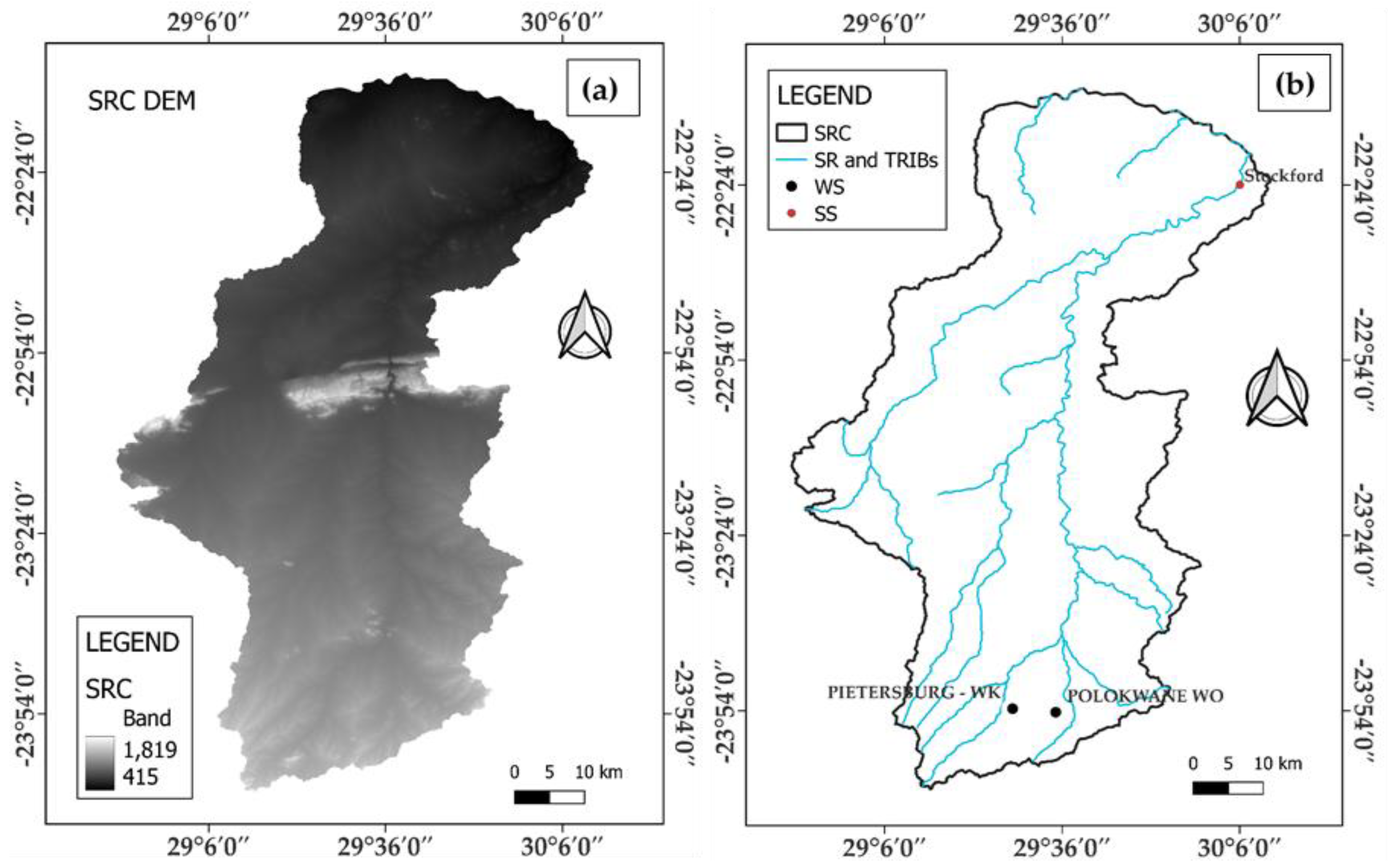
2.1. Study Area Description

The Sand River Catchment (SRC) is a right-side tributary of the Limpopo River, found at 22°50′54″ S and 29°38′01″ E. The Sand River Catchment is located at the north–central part of Limpopo province, South Africa, with the source located in Ysterberg, in the Waterberg District Municipality of Mogalakwena in Limpopo (Figure 1). It flows northwards through central Limpopo, cutting through the Soutpansberg across the deep gorge, Waterpoort. It then joins the Limpopo River on the right bank, 7 km east of Musina [31]. It covers the entire Vhembe District Municipality (Makhado and Musina Local Municipalities) and Capricorn District Municipality (Polokwane, Molemole, and Blouberg Local Municipalities) [32]. According to Kapangaziwiri et al. [31], the climate of the SRC is extremely arid, with an average temperature of 20 °C, a maximum temperature of 30 °C, and a minimum temperature of 4 °C; precipitation is seasonal, with the most taking place in summer. The total annual precipitation ranges between 300 mm and 700 mm, with the average annual evaporation dependent on the amount of precipitation. The average annual run-off is 86.5 m³ [20]. The SRC has a gross area of 15,769 km², which is made up of tertiary catchment area 71 with a gross area of 13,307 km² and area 72 with a gross area of 3462 km² and an overall length of 350 km. The topography of the catchment is flat with an elevation of 418 m [32]. The SRC is a dry catchment consisting of limited surface water resources. The study performed by the Department of Water and Sanitation (DWS) [20] found that the SRC has water reserves as groundwater, which are extremely over-exploited because of agricultural irrigation. Agriculture is the largest water user within the catchment due to increasing irrigation demand.

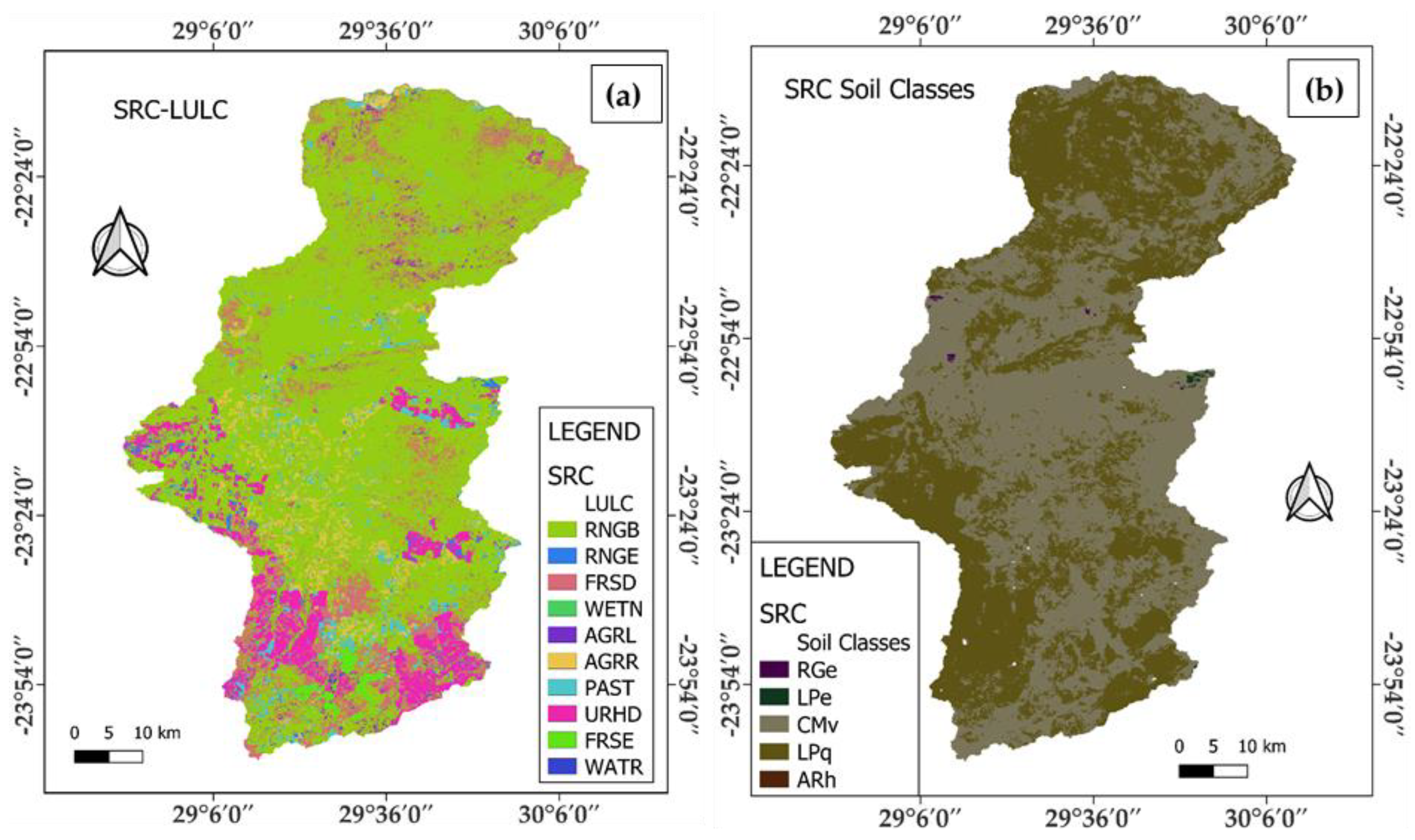
2.2. SWAT+ Input Data

SWAT+ works on the concept of Hydrological Response Units (HRUs). These are unique combinations of different layers, such as landscape unit, land use–land cover (LULC), soil classes, and slope classes derived from the Digital Elevation Model (DEM) [33]. The 30-metre spatial resolution of the DEM for the SRC as the Shuttle Radar Topography Mission (SRTM) was obtained from the United States Geological Survey (https://earthexplorer.usgs.gov/, accessed on 14 April 2024) (Figure 2a). The 20 m spatial resolution LULC raster shapefile was obtained from the Department of Forestry, Fisheries, and the Environment, South African national land cover (SANLC) raster shapefile of 2020 (https://za.africageoportal.com/maps/cff4e27fa6fb46f6bde59edb889398ef/explore?location=-24.511888%2C29.486534%2C6.98, accessed on 27 April 2024) (Figure 3a and

Table 1. Conversion of SANLC LULC classes to SWAT+ LULC classes.

SANLC LULC Classes	SWAT+ LULC Classes	SWAT+ LULC Description
Grasslands	RNGE	Grasslands/Herbaceous
Shrubland	RNGB	Range Shrubland
Buildings (residential, industries, and mines)	URHD	Urban High Density
Cultivated land	AGRL	Generic
Indigenous forest	FRSE	Evergreen Forest
Waterbodies	WATR	Water
Pivot irrigated land	AGRR	Row Crops
Non-pivot land	PAST	Pasture
Planted forest	FRSD	Deciduous Forest
Wetlands	WETN	Emergent Wetlands

). The soil data was extracted from the digital soil map of the world obtained from the International Soil Reference and Information Centre World Soil Information(https://data.isric.org/geonetwork/srv/eng/catlog.search#/metadata/f9a3a4e0-27a8-4acc-861f-26c112699c3e, accessed on 28 April 2024) with a 250 m resolution (Figure 3b and

Table 2. Main soil classes distributed within SRC.

Soil Texture	Name	Soil Code
Loamy Clay	Lithic Leptosols	LPq
Sandy Clay–Loam	Vertic Cambisols	CMv
Clay	Calcaric Regosols	RGe
Loam	Eutric Leptosols	LPe
Loamy Sand	Haplic Arenosols	ARh

). To identify the major soil classes, the use of soil data with a low spatial resolution is acceptable [30]. Low spatial resolution remote sensing captures a large region and provides data by analysing the spectral frequencies discounted by higher resolution procedures, regardless of the lack of preciseness [34]. The meteorological data needed for SWAT+ simulations in this study, such as daily precipitation, maximum/minimum temperatures, wind speed, solar energy, and relative humidity, was obtained from the South African Weather Service (SAWS) (Weather Stations: 0677802BX and 0677802A5). The water quality data required for calibration and validation of the SWAT+ model (Total Inorganic Nitrogen (TIN), Total Inorganic Phosphorus (TIP), and sediment) was obtained from the DWS Resource Quality Information System (RQIS) (Sampling Station: 07H005Q01, Stockford).

2.3. SWAT+ Setup and Procedure

The SWAT+ (SWAT+ rev. 61) was used via the QSWAT+ interface embedded in QGIS 3.32.0 software. This study adopted the SWAT+ setup described by Bieger et al. [30]. The SWAT+ setup comprises four major steps, namely, delineating the watershed, creating HRUs, editing the input, and running SWAT+, then visualising is conducted [24]. The SRC was delineated by incorporating DEM and river network data into QSWAT+. The outlet of the river was accurately drawn on the mouth of the river. Multiple HRUs were created by assimilating the LULC map, soil texture map, LULC table, and soil table into the QSWAT+ interface. The catchment was divided into nine sub-catchments and 1088 HRUs, which were all considered in the current assessment. Daily meteorological data and weather station files were uploaded into the SWAT+ editor to ensure the accurate simulation of hydrological processes in the catchment as indicated by Bieger et al. [30]. The LULC and soil tables were converted to comma-separated value (CSV) files, and meteorological data was converted to text (UTF-8) files to enable QSWAT+ and SWAT+ editor data processing. Thereafter, monthly and annual TIN [ammonium (NH₄⁺) + nitrates (NO₃⁻) + nitrites (NO₂⁻)] and TIP and sediment loads were visualised at the catchment level. The accurate simulations of TIN, TIP, and sediment were based on theoretical SWAT+ considerations, as described by Bieger et al. [30]. The hydrological components of SWAT+ simulations in this study were determined by using the water balance equation (Equation (1) [24]).

$${\mathrm{SW}}_{\mathrm{t}} = {\mathrm{SW}}_0 + {\sum }_{\mathrm{i}=1}^{\mathrm{t}}\left({\mathrm{R}}_{\mathrm{d}\mathrm{a}\mathrm{y}}-{\mathrm{Q}}_{\mathrm{s}\mathrm{u}\mathrm{r}\mathrm{f}}-{\mathrm{E}}_{\mathrm{a}}-{\mathrm{W}}_{\mathrm{s}\mathrm{e}\mathrm{e}\mathrm{p}}-{\mathrm{Q}}_{\mathrm{g}\mathrm{w}}\right)$$

(1)

where SW_t—final state of the water content in the soil (mm H₂O), SW₀—initial state of the water content in the soil (mm H₂O), i—specific day, t—given time (days), R_day—the sum of precipitation per day, Q_surf—the sum of runoff per day, E_a—the sum of evapotranspiration per day, W_seep—the sum of water entering the vadose zone from the soil profile per day, and Q_gw—the sum of return flow per day.

2.4. SWAT+ Calibration and Validation

The SWAT+ model was calibrated and validated using the monthly observed TIN, TIP, and sediment loads from the outlet of the catchment (Figure 2b, Sampling Station: 07H005Q01). The calibration and validation period of the model was dependent on the availability of data. SWAT+ simulation was conducted for the period October 1990 to September 2022 (water years). The model warm-up was set up for the period from October 1990 to September 1992 and it was calibrated from January 1998 to December 2001. It was then validated for the period from January 2002 to December 2005 for the observed monthly TIN, TIP, and sediment loads (Figure 4). Prior to the calibration of the model, a sensitivity analysis was conducted. The purpose of the analysis of sensitivity was to select the most sensitive variables that affect TIN, TIP, and sediment outputs for the calibration of the model [31]. Moreover, the accuracy of the simulated outputs against the observed data was assessed using the three statistical indices, such as the Nash–Sutcliffe efficiency (NSE) index, the coefficient of determination (R²), and the percent bias (PBIAS) (Equations (2)–(4)) [24,25,26,27,28,29,30].

$$\mathrm{NSE}=1 – {\displaystyle \frac{{\sum }_{\mathrm{i}=1}^{\mathrm{n}}{\left({\mathrm{Q}}_{\mathrm{s},\mathrm{i}}-{\mathrm{Q}}_{\mathrm{o},\mathrm{i}}\right)}^2}{{\sum }_{\mathrm{i}=1}^{\mathrm{n}}{\left({\mathrm{Q}}_{\mathrm{o},\mathrm{i}}-{\mathrm{Ǭ}}_{\mathrm{o}}\right)}^2}}$$

(2)

$${\mathrm{R}}^2={\displaystyle \frac{[{\sum }_{\mathrm{i}=1}^{\mathrm{n}}{\left({\mathrm{Q}}_{\mathrm{o},\mathrm{i}}-{\mathrm{Ǭ}}_{\mathrm{o}}\right)\left({\mathrm{Q}}_{\mathrm{s},\mathrm{i}}-{\mathrm{Ǭ}}_{\mathrm{s}}\right)]}^2}{{\sum }_{\mathrm{i}=1}^{\mathrm{n}}{\left({\mathrm{Q}}_{\mathrm{o},\mathrm{i}}-{\mathrm{Ǭ}}_{\mathrm{o}}\right)}^2{\sum }_{\mathrm{i}=1}^{\mathrm{n}}{\left({\mathrm{Q}}_{\mathrm{s},\mathrm{i}}-{\mathrm{Ǭ}}_{\mathrm{s}}\right)}^2}}$$

(3)

$$\mathrm{PBIAS}={\displaystyle \frac{\sum _{\mathrm{i}-1}^{\mathrm{n}}\mathrm{Q}\mathrm{o}.\mathrm{i}-\sum _{\mathrm{i}-1}^{\mathrm{n}}\mathrm{Q}\mathrm{s},\mathrm{i}}{\sum _{\mathrm{i}-1}^{\mathrm{n}}\mathrm{Q}\mathrm{o},\mathrm{i}}} \times 100$$

(4)

where n—number of observations, Q_o,i—observed value at the specific time, Q_s,i—simulated value at the specific time, i—specific time, Ǭ_o—mean of observed values, and Ǭ_s—mean of simulated values.

The SWAT+ toolbox consists of four sensitivity analysis methods, namely, random balance design, Fourier amplitude, Sobol, delta moment independent measures, and Fourier amplitude [35]. In this study, the Sobol sensitivity analysis method and auto-calibration were employed to examine the sensitive parameters and parameter values to achieve significant model performance. The Sobol sensitivity analysis method directly calculates the sensitivity index of the SWAT+ parameters to be used to evaluate the reliability of the simulated outputs and reduces uncertainties [36]. The sensitivity analysis was performed using the global analysis method to reduce the number of simulations as compared to the local analysis (one-at-a-time). The seed value was set to 25, generating 250 samples. The seed value determines the number of samples to be generated by the SWAT+ toolbox during the sensitivity analysis [30].

The Sobol procedure uses the theory of variance decomposition whereby the interaction between SWAT+ parameters is based on the decomposition of total variance. If p = q(x) = (x₁, x₂…x_m), where x₁, x₂…x_m is the structure of the model and m is the number of SWAT+ parameters, then Equation (5) expresses how variance decomposition was calculated. The indices of the first (Sp), second (Spr), and total (STp) order of sensitivity were calculated using Equations (6)–(8). The difference between STp and Sp was utilised to assess the mutual effect between the pth parameter and other parameters in SWAT+ using Equation (9) [33].

$$\mathrm{Z}(\mathrm{p})={\sum }_{\mathrm{p}=1}^{\mathrm{m}}{\mathrm{Z}}_{\mathrm{p}}+{\sum }_{\mathrm{p}<\mathrm{r}}^{\mathrm{m}}{\mathrm{Z}}_{\mathrm{p}\mathrm{r}}+\dots +{\mathrm{Z}}_{\mathrm{1,2},\dots ,\mathrm{M}}$$

(5)

where Z(p)—total variance of the SWAT+ output p, Z_p—variance term of the pth parameter, Z_pr—variance term of the joint action of the pth and rth parameters, and Z_1,2,…,M—the variance term of the interaction of all parameters.

$${\mathrm{S}}_{\mathrm{p}}={\displaystyle \frac{{\mathrm{Z}}_{\mathrm{p}}}{\mathrm{Z}\left(\mathrm{p}\right)}}$$

(6)

$${\mathrm{S}}_{\mathrm{pr}}={\displaystyle \frac{{\mathrm{Z}}_{\mathrm{p}\mathrm{r}}}{\mathrm{Z}\left(\mathrm{p}\right)}}$$

(7)

$${\mathrm{S}}_{\mathrm{Tp}}=1-{\displaystyle \frac{{\mathrm{Z}}_{-\mathrm{p}}}{\mathrm{Z}\left(\mathrm{p}\right)}}$$

(8)

MN_p = S_Tp − S_p

(9)

where S_p and S_pr—influence of an individual parameter and the combination of two parameters on SWAT+ output, S_Tp—influence on the combination of SWAT+ parameters, Z_−p—variance without the effect of the pth parameter, and MN_p—interaction effect of the pth SWAT+ parameter [33].

The simulated output from the sensitivity analysis can be utilised to remove the parameters that are non-sensitive during the calibration procedure [35]. The results obtained from the global sensitivity analysis are presented in

Table 3. The list of the sensitive parameters obtained during sensitivity analysis in this study. These parameters are presented based on their level of sensitivity which measures their contribution to the transportation of sediment, TIN, and TIP loads.

Variable	Parameter	Definition	Sensitivity
Sediment	usle_p	Universal soil loss equation support practice factor	0.93
	usle_k	Universal soil loss equation soil erodibility factor	0.91
	rock	Rock fragment content (total weight %)	0.80
	slope	Average slope steepness in HRU (m/m)	0.69
TIN (NO3−, NO2−, and NH4+)	anion-excl	Fraction of porosity from which anions are excluded	0.89
	nperco	Nitrogen percolation coefficient	0.77
	biomix	Biological mixing efficient	0.12
TIP	bd	Moist bulk density (Mg/m3)	0.71
	pperco	Phosphorus percolation coefficient	0.46
	phoskd	Phosphate soil partitioning coefficient	0.28

. Global sensitivity analysis quantifies the impact of various sources of uncertainty, such as model parameters, on model output uncertainty [30]. The non-sensitive parameters were filtered during the calibration of the SWAT+ model as they had no impact on the simulation of nutrients and sediments [37]. The values of the most sensitive parameters for nutrients and sediments were deduced by Sobol sensitivity analysis and presented based on the level of sensitivity per variable. Sobol sensitivity analysis aims to decompose the variance of a model’s output into contributions from each input parameter and their interactions [36]. It provides a quantitative measure of how changes in input variables affect the uncertainty in the output variable [36]. The most sensitive parameter for TIN (NH₄⁺, NO₃⁻, NO₂⁻) is anion_excl; for TP, it is bd; and for sediment, it is usle_p.

The SWAT+ model is able to calibrate the TIN, TIP, and sediment loads as well as to prioritise the parameters that influence hydrological processes [38]. The model was calibrated and validated using the Dynamically Dimensioned Search (DDS) algorithm with maximum iterations set to 500 and NSE set as an objective function. DDS is a straightforward, stochastic, single-solution-based heuristic global search technique that dynamically modifies the dimensions of the search space to identify good solutions to optimise problems, particularly ones with numerous parameters [39]. This algorithm was embedded into the SWAT+ toolbox and used in auto calibration.

The sensitive parameters listed in

Table 4. The results obtained during the calibration of the SWAT+ model with the observed data of sediment, TIN, and TIP using the sensitive parameters.

Parameters	Object	Change Type	Min-Value	Calibrated Value	Max-Value	Units
anion-excl	sol	Percent	0.1	0.69	0.90
Nperco	bsn	Percent	0	0.52	1
Biomix	hru	Percent	0	0.23	1
Bd	sol	Percent	0.90	1.60	2.50	Mg/m3
Pperco	bsn	Percent	10	11.40	17.50
Phoskd	bsn	Percent	100	147	200
usle_p	hru	Percent	0	0.38	1
Rock	sol	Percent	0	48	100	%
Slope	hru	Percent	0.0001	0.23	0.90	m/m
usle_k	sol	Percent	0	0.51	0.65

Note: bsn—basin, hru—hydrological response unit, and sol—soil.

were adjusted when the SWAT+ model was calibrated with the observed TIN (NH₄⁺, NO₃⁻, NO₂⁻), TIP, and sediment data to evaluate the performance of the model. It was important to perform sensitivity analysis, as the sensitive parameters played a huge role in determining the ability of the model to effectively simulate the influence of hydrological processes in the transportation of nutrients and sediments. As such, there was a need to utilise sensitive parameters with the calibrated values throughout the simulations. The calibrated SWAT+ model with observed TIN, TIP, and sediment data from the outlet (mouth) of the SRC considered ten sensitive parameters that affected the hydrological processes in the catchment (Table 4).

The simulated sediment, TIN, and TIP loads showed that the model output accurately simulated the observed data. Statistical indices were used to evaluate SWAT+ performance, which showed an agreement between the observed data and the simulated output. The obtained results showed that all the statistical indices for SWAT+ model performance during calibration and validation (NSE and R² ≥ 0.72; −17.30 ≤ PBIAS ≤ 14.74) were within an acceptable range as described by [4,5,6,7,8,9,10,11,12,13,14,15,16,17,18,19,20,21,22,23,24]. In other words, SWAT+ model statistical indices prescribed an agreement between the observed data and the simulated output in this study. For sediments, the PBIAS was found to be −1.11 during calibration and −17.30 during validation, indicating that there was an overestimation of sediment load of 1.11% and 17.30%, respectively. For all other variables, the PBIAS (1.65 ≤ PBIAS ≤ 14.74) indicated that there was an underestimation during calibration and validation. The indicators of the agreement between the observed data and simulated outputs during calibration and validation are presented in Figure 4.

2.5. SWAT+ Application

The calibrated and validated SWAT+ model was used to simulate monthly and annual TIN, TIP, and sediment loads in the SRC from October 1992 to September 2022. Moreover, spatial variability maps for TIN, TIP, and sediment loads were printed from the QSWAT+. The spatial variabilities of sediment, TIN, and TIP loads were compared for the high precipitation and temperature month (January) and the low precipitation and temperature month (July) to assess the impact of high and low precipitation and temperature peaks on the sediment, TIN, and TIP loads and to evaluate the loading variation during the simulation period. To do this, three variability maps for each month for the 1993-, 2007-, and 2022-year intervals were generated and incorporated into one map, and the load variabilities were assessed.

2.6. Statistical Analysis

The coefficient of determination (R²) in linear regression was used to determine the proportion of variance in the dependent variables that can be explained by the independent variables. Consequently, the dependence of sediment, TIN, and TIP loads on precipitation and temperature was determined by the R² through linear regression analysis. The value of R² ranged between 0 and 1; the closer the R² value was to 1, the stronger the dependence of sediment, TIN, and TIP loads on precipitation and temperature [40]. The F test for the overall levels of significance of the model output was conducted to show if there was a linear relationship between the dependent (sediment, TIN, and TIP loads) and the independent (precipitation and temperature) variables [40,41]. To do this, the F statistics in the one-way analysis of variance (ANOVA) were determined to deduce the level of significance of the relationship between dependent and independent variables. The statistical analysis was conducted at a 5% significance level and 95% confidence level using the Excel add-in XLSTAT (2023 version).

3. Results

3.1. Impact of Precipitation and Temperature Variation on Monthly Sediment Load

The SRC’s average monthly precipitation and temperature showed a variable pattern of impact on average sediment load. When the average monthly precipitation and temperature increased, the average monthly sediment load increased and vice versa (Figure 5). High average monthly sediment loads were simulated in the summer months, with an average load of 112.8 ton/mo. in December, 100.8 ton/mo. in January, and 75.6 ton/mo. in February at average monthly precipitation/temperatures of 96.8 mm/22.9 °C, 83.1 mm/23.4 °C, and 68.7 mm/23.3 °C. In autumn, the sediment load began to decrease as the precipitation and temperature decreased. The simulated average monthly sediment load during the autumn season in relation to average monthly precipitation and temperature was 66.0 ton/mo. in March, 48.0 ton/mo. in April, and 36.0 ton/mo. in May with precipitation/temperatures of 52.6 mm/22.1 °C, 31.3 mm/19.4 °C, and 11.2 mm/16.4 °C, respectively.

The lowest average monthly sediment loads were simulated in the winter months, with an average of 33.6 ton/mo. in June, 32.4 ton/mo. in July and 26.4 ton/mo. in August with average monthly precipitation/temperatures of 2.3 mm/13.5 °C, 2.3 mm/13.1 °C, and 1.6 mm/15.7 °C. In spring, the average monthly sediment load began to increase in the Sand River. The average loads were 44.4 ton/mo. in September, 49.2 ton/mo. in October, and 103.2 ton/mo. in November with average monthly precipitation/temperatures of 4.8 mm/19.2 °C, 38.9 mm/21.1 °C, and 88.9 mm/22.0 °C, respectively. The results further showed a perfect correlation (0.95) between the average monthly precipitation and average monthly sediment load and a good correlation between average monthly temperature and average monthly sediment load (0.68), as shown in

Table 5. Statistical summary for the analysis of variance between monthly average precipitation and temperature and the sediment load.

Variables	R2	Source	DF	Sum of Squares	Mean Squares	F	Pr > F	p-Value Signification Codes
Precipitation	0.95	Model	1	9770	9770	200	<0.0001	***
vs.		Error	10	489	49
Sediment		Corrected Total	11	10,260
Temperature	0.68	Model	1	7020	7020	22	0.001	***
vs.		Error	10	3240	324
Sediment		Corrected Total	11	10,260

Note: Signification codes: 0 < *** < 0.001.

. Furthermore, the p-value (p < 0.05) of the F statistic deduced during ANOVA analysis shows the statistical significance of the relationship between average monthly precipitation, temperature, and sediment load in the SRC.

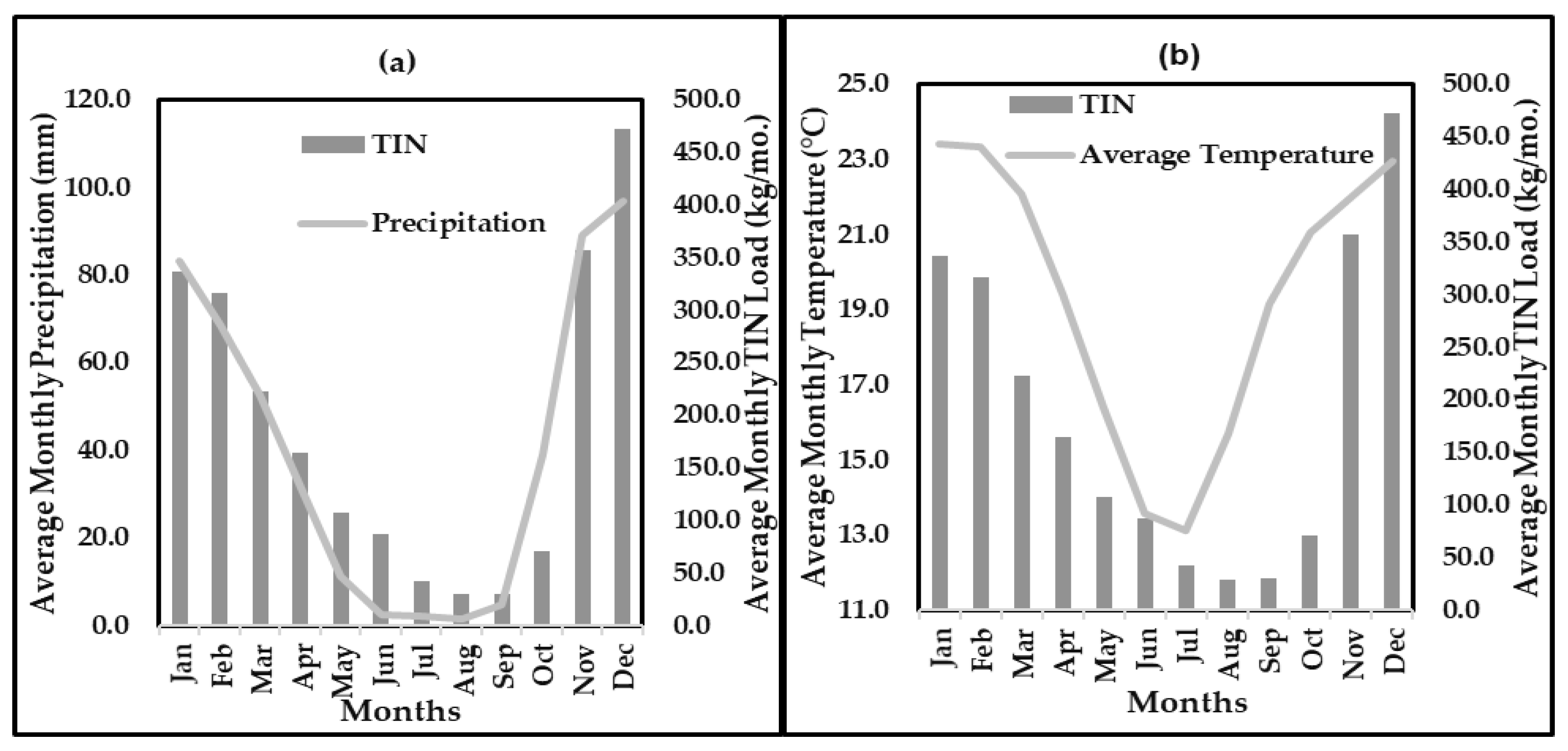
3.2. Impact of Precipitation and Temperature Variation on Monthly TIN Load

The intra-annual variation in TIN load results deduced from the average monthly graphical presentation shows that the average monthly TIN load in the Sand River increased and decreased with an increase and decrease in average monthly precipitation and temperature (Figure 6a,b). However, the greatest agreement in TIN load in relation to climate parameters is observed in Figure 6a (impact of precipitation on average monthly TIN load) compared to Figure 6b (impact of temperature on average monthly TIN load). The highest average monthly TIN loads were simulated in summer, with an average load of 471.9 kg/mo. in December, 336.5 kg/mo. in January, and 315.5 kg/mo. in February, with average monthly precipitation/temperatures of 96.8 mm/22.9 °C, 83.1 mm/23.4 °C, and 68.7 mm/23.3 °C, respectively. In autumn, the simulated average monthly TIN in relation to average monthly precipitation and temperature was 222.0 kg/mo. in March, 164.2 kg/mo. in April, and 107.7 kg/mo. in May, with precipitation/temperatures of 52.6 mm/22.1 °C, 31.3 mm/19.4 °C, and 11.2 mm/16.4 °C.

The lowest average monthly TIN load was simulated in winter with an average of 87.2 kg/mo. in June, 42.2 kg/mo. in July, and 29.2 kg/mo. in August, with average monthly precipitation/temperatures of 2.3 mm/13.5 °C, 2.3 mm/13.1 °C, and 1.6 mm/15.7 °C. In spring, the average monthly TIN load began to increase in the Sand River. The average monthly TIN loads were 29.8 kg/mo. in September, 70.6 kg/mo. in October, and 356.6 kg/mo. in November, with average monthly precipitation/temperatures of 4.8 mm/19.2 °C, 38.9 mm/21.1 °C, and 88.9 mm/22.0 °C. The results further show a perfect correlation (0.91) between the average monthly precipitation and average monthly TIN load and a strong correlation between average monthly temperature and average monthly TIN load (0.59), as shown in

Table 6. Statistical summary for the analysis of variance between monthly average precipitation and temperature and TIN load.

Variables	R2	Source	DF	Sum of Squares	Mean Squares	F	Pr > F	p-Value Signification Codes
Precipitation	0.91	Model	1	229,155	229,155	105	<0.0001	***
vs.		Error	10	21,768	2177
TIN		Corrected Total	11	250,923
Temperature	0.59	Model	1	146,866	146,866	14	0.004	**
vs.		Error	10	104,057	10,406
TIN		Corrected Total	11	250,923

Note: Signification codes: 0 < *** < 0.001 < ** < 0.01.

. Furthermore, the p-value (p < 0.05) of the F statistic deduced during ANOVA analysis shows the statistical significance of the relationship between average monthly precipitation and temperature and the average monthly TIN load.

3.3. Impact of Precipitation and Temperature Variation on Monthly TIP Load

The average monthly precipitation showed a greater variation pattern with average monthly TIP load compared to average monthly temperature (Figure 7). The highest average monthly TIP loads were simulated in summer, with an average load of 146.2 kg/mo. in December, 171.6 kg/mo. in January, and 136.2 kg/mo. in February, with average monthly precipitation/temperatures of 96.8 mm/22.9 °C, 83.1 mm/23.4 °C, and 68.7 mm/23.3 °C, respectively. In autumn, the TIP load began to decrease as the precipitation and temperature were decreasing. The simulated average monthly TIP load during the autumn season in relation to average monthly precipitation and temperature was 103.5 kg/mo. in March, 79.1 kg/mo. in April, and 61.5 kg/mo. in May, with precipitation/temperatures of 52.6 mm/22.1 °C, 31.3 mm/19.4 °C, and 11.2 mm/16.4 °C.

The lowest average monthly TIP loads were simulated in winter with an average of 45.3 kg/mo. in June, 13.2 kg/mo. in July, and 11.0 kg/mo. in August, with average monthly precipitation/temperatures of 2.3 mm/13.5 °C, 2.3 mm/13.1 °C, and 1.6 mm/15.7 °C. In spring, the average monthly TIP load began to increase in the Sand River. The average monthly TIP loads were 11.3 kg/mo. in September, 77.7 kg/mo. in October, and 125.8 kg/mo. in November, with average monthly precipitation/temperatures of 4.8 mm/19.2 °C, 38.9 mm/21.1 °C, and 88.9 mm/22.0 °C. The statistical analysis further shows the perfect correlation (0.89) between the average monthly precipitation and average monthly TIP load and a very strong correlation between average monthly temperature and average monthly TIP load (0.71), as shown in

Table 7. Statistical summary of the analysis of variance between monthly average precipitation and temperature and TIP load.

Variables	R2	Source	DF	Sum of Squares	Mean Squares	F	Pr > F	p-Value Signification Codes
Precipitation		Model	1	30,388	30,388	83	<0.0001	***
vs.	0.89	Error	10	3658	366
TIP		Corrected Total	11	34,046
Temperature		Model	1	24,215	24,215	25	0.001	***
vs.	0.71	Error	10	9831	983
TIP		Corrected Total	11	34,046

Note: Signification codes: 0 < *** < 0.001.

. Furthermore, the p-value (p < 0.05) of the F statistic deduced during ANOVA analysis shows the statistical significance of the relationship between average monthly precipitation and temperature and the average monthly TIP sediment load.

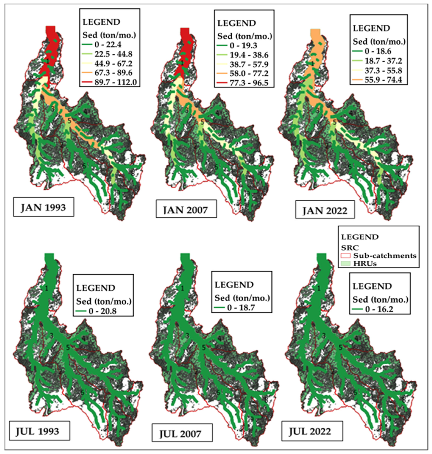
3.4. Long-Term Spatio-Temporal Variability of Sediment, TIN, and TIP Loads During High and Low Peaks of Precipitation and Temperature in the SRC

There is a clear indication of the impact of precipitation and temperature variation on the sediment, TIN, and TIP loads in the SRC, as shown by the results above. The sediment, TIN, and TIP loads vary based on the seasonal changes in temperature and precipitation, where the highest peaks are experienced in summer and the lowest peaks are experienced in winter. In Figure 8, Figure 9 and Figure 10, the long-term spatial variation maps of sediment, TIN, and TIP loads for the months of January and July at the beginning (1993), middle (2007), and end (2022) of the 30-year simulation period are shown. The spatio-temporal maps show that the highest sediment, TIN, and TIP loads were simulated in January, while the lowest loadings occurred in July in the SRC. Furthermore, the spatio-temporal variation maps show that the sediment, TIN, and TIP loads have been decreasing drastically over the past 30 years; the highest load captured occurred in 1993 (112.0 ton/mo., 462.0 kg/mo., and 188.0 kg/mo.), then it decreased in 2007 (96.5 ton/mo., 407.0 kg/mo., and 166.5 kg/mo.) and further decreased in 2022 (74.4 kg/mo., 308.2 kg/mo., and 130.6 kg/mo.), with the lowest TIP load in July following the same pattern (20.8 ton/mo., 89.6 kg/mo., and 36.1 kg/mo.), (18.7 ton/mo., 77.8 kg/mo., and 31.2 kg/mo.), and (16.2 ton/mo., 68.2 kg/mo., and 28.4 kg/mo.), respectively. As shown in the spatial variation maps, the sediment, TIN, and TIP loads are found to be high at the mouth of the Sand River compared to the headwater of the SRC during the mid-summer (January). This could be linked to the transportation of sediment and nutrient loads by the river resulting from the increased runoff from agricultural farmlands during high precipitation.

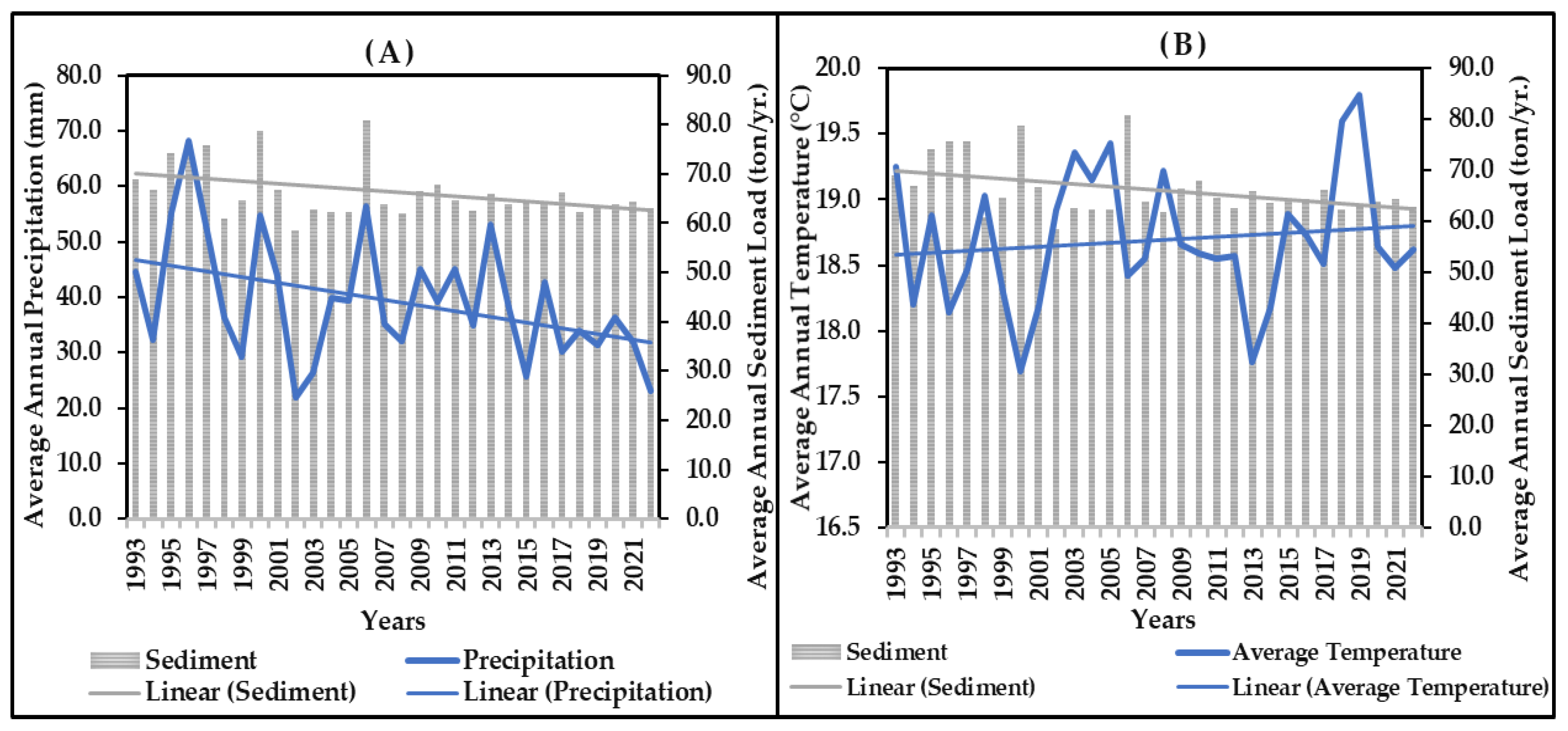
3.5. Inter-Annual Impact of Precipitation and Temperature on Annual Sediment Load

The simulated average annual sediment load from October 1992 to September 2022 showed a direct relationship with average annual precipitation; however, it displayed an indirect relationship with average annual temperature. As average annual precipitation decreased throughout the simulation period, the average annual sediment load also decreased. Conversely, when the average annual temperature increased, there was a decrease in sediment load (Figure 11). The results further show a very strong correlation (0.63) between average annual precipitation and average annual sediment load and a moderate correlation between average annual temperature and average annual sediment load (0.23), as shown in

Table 8. Statistical summary of the analysis of variance between annual average precipitation and temperature and the sediment load.

Variables	R2	Source	DF	Sum of Squares	Mean Squares	F	Pr > F	p-Value Signification Codes
Precipitation		Model	1	545	545	48	<0.0001	***
vs.	0.63	Error	28	316	11
Sediment		Corrected Total	29	861
Temperature		Model	1	195	195	8	0.008	**
vs.	0.23	Error	28	666	24
Sediment		Corrected Total	29	861

Note: Signification codes: 0 < *** < 0.001 < ** < 0.01.

. Furthermore, the p-value (p < 0.05) of the F statistic deduced during ANOVA analysis shows the statistical significance of the relationship between average annual precipitation and temperature and the average annual sediment load.

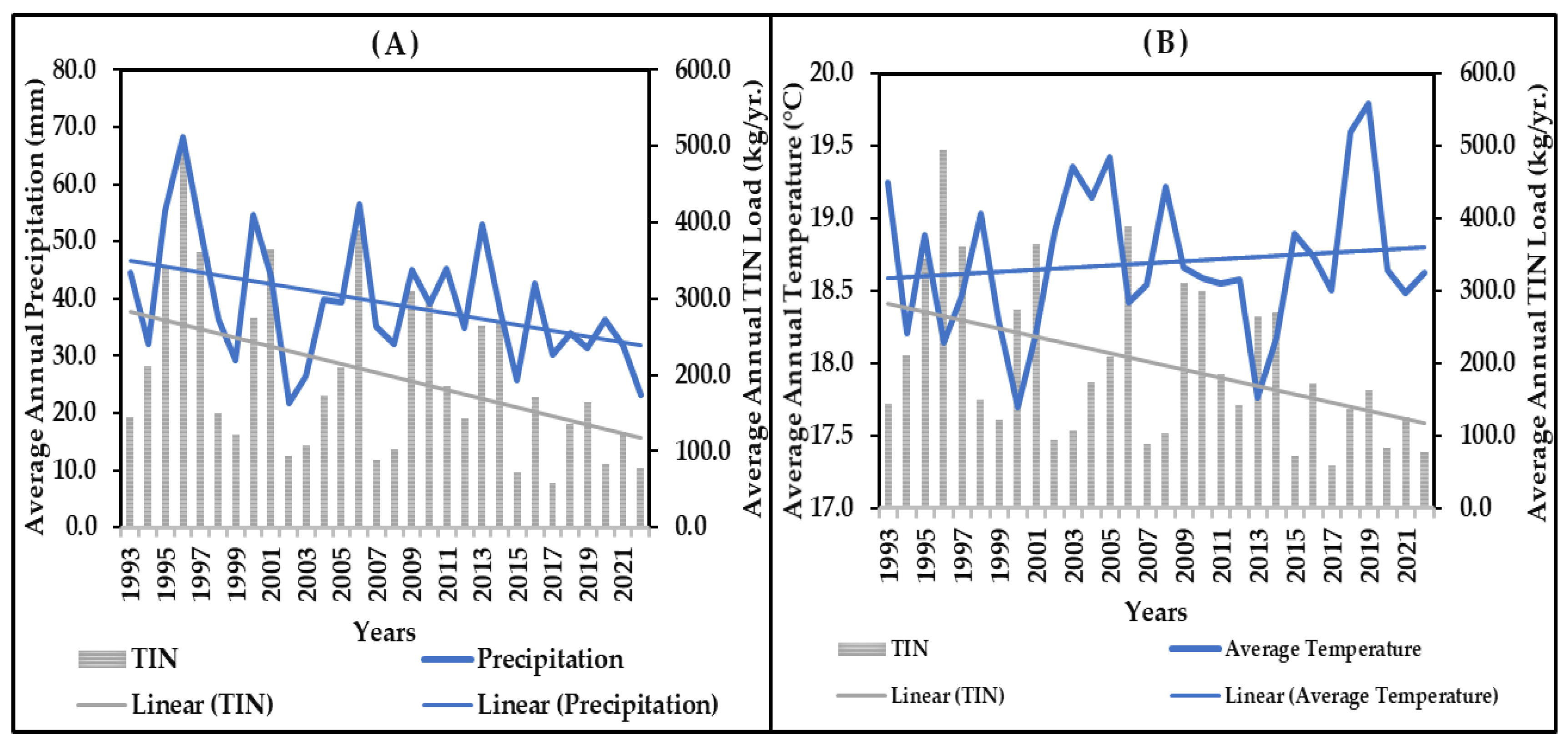
3.6. Inter-Annual Impact of Precipitation and Temperature on Annual TIN Load

The simulated average annual TIN load decreased drastically from October 1992 to September 2022 (Figure 12). The observed decrease in the average annual TIP load was related to a decrease in average annual precipitation. However, the results indicated that decreases in average annual temperature in the SRC during the winter months resulted in an increase in annual average TIN load. The results obtained showed that the average annual TIP load depended on average annual precipitation as compared to average annual temperature. The analysis of variance confirmed a variation relationship whereby there was a very strong correlation (0.73) between the average annual precipitation and average annual TIN load and a weak correlation between average annual temperature and average annual TIN load (0.19), as shown in

Table 9. Statistical summary of the analysis of variance between annual average precipitation and temperature and the TIN load.

Variables	R2	Source	DF	Sum of Squares	Mean Squares	F	Pr > F	p-ValuesSignification Codes
Precipitation		Model	1	270,052	270,052	77	<0.0001	***
vs.	0.73	Error	28	97,848	3495
TIN		Corrected Total	29	367,900
Temperature		Model	1	65,367	65,367	6	0.020	*
vs.	0.19	Error	28	302,533	10,805
TIN		Corrected Total	29	367,900

Note: Signification codes: 0 < *** < 0.001 < * < 0.05.

. Furthermore, the p-value (p < 0.05) of the F statistic deduced during ANOVA analysis shows the statistical significance of the relationship between average annual precipitation and temperature and the average annual TIN load.

3.7. Inter-Annual Impact of Precipitation and Temperature on Annual TIP Load

The results of the 30-water-years (October 1992 to September 2022) simulated average annual TIP load showed that there was a direct relationship with average annual precipitation (Figure 13) and that the observed decrease in average annual precipitation influenced the decrease in average annual TIP load in the SRC. However, the average annual TIP load decreased with an increase in average annual temperature, indicating an inverse relationship. The results further show a strong correlation (0.55) between the average annual precipitation and average annual TIP, but a weak correlation between average annual temperature and average annual TIP load (0.05), as shown in

Table 10. Statistical summary of the analysis of variance between annual average precipitation and temperature and the TIP load.

Variables	R2	Source	DF	Sum of Squares	Mean Squares	F	Pr > F	p-ValuesSignification Codes
Precipitation		Model	1	2788	2788	34	<0.0001	***
vs.	0.55	Error	28	2301	82
TIP		Corrected Total	29	5089
Temperature		Model	1	258	258	1	0.232	°
vs.	0.05	Error	28	4832	173
TIP		Corrected Total	29	5089

Note: Signification codes: 0 < *** < 0.001 < ° < 1.

. Furthermore, the p-value (p < 0.05) of the F statistic deduced during ANOVA analysis shows the statistical significance of the relationship between average annual precipitation and average annual TIP load. The relationship between the average annual temperature and average annual TIP load was deduced to be statistically insignificant (p > 0.05) during ANOVA analysis.

4. Discussion

4.1. Impact of Monthly Precipitation and Temperature on Agricultural NPS Pollution

The broader Limpopo River basin, out of which the SRC is carved, is known to have low precipitation and to record high hydroclimatic extremes, characterised by drought, floods, and temperature variations [42,43]. The spatio-temporal variability in the SRC climate observed in the current study can therefore be linked to this, leading to the water quantity and quality stress that has been experienced in the SRC [44]. These cumulative stressors negatively impact agricultural activities in the catchment, leading to the extensive use of fertilisers for soil nutrient enrichment and irrigation to improve crop yield in the spring and summer months [44]. The results of the current study confirmed this variation pattern; they showed that average monthly sediment, TIN, and TIP loads followed the same variation pattern as the average monthly precipitation and temperature variation (Figure 5, Figure 6 and Figure 7) in the catchment. The discharge loads of sediment, TIN, and TIP reached the highest peaks in summer months (December, January, and February) and the lowest peaks in winter (June, July, and August). This can be linked to rainfed spring farming operations, where tillage activities are conducted extensively on the farmlands to prepare for planting in summer [45].

Usually, farmlands in this area are dominated by weeds; conventional tillage is usually conducted to prevent plant-weed competition [45]. Conventional tillage often increases the sediment yield in the agricultural farmlands that are subject to soil erosion [46]. During the preparation for planting in the SRC spring months of September–October, TIN and TIP are introduced to the soil through fertiliser application, crop residue application, and manure application [45]. As a result, the yields of sediment, TIN, and TIP through runoff into the SRC increase during high precipitation (in summer). This also occurs through intensified irrigation, leading to the increased transportation of the TIN, TIP, and sediment loads. Irrigation intensification is necessary in several instances when there is a delay in the onset of rainfall [47]. In addition, Costa et al. [48] and Zhang et al. [49] indicated that the chemical properties of nitrogen and phosphorus constituents allow them to be sorbed (absorbed–adsorbed) by sediments, influencing nutrient dynamics in the river catchments. This further supports the similar response of sediment, TIN, and TIP loads towards precipitation variation in the SRC, based on the findings of this study.

The average monthly sediment, TIN, and TIP loads are relatively low in winter, according to Eccles et al. [50]; this could be linked to low precipitation during these months, thereby leading to low agricultural runoff. Shikwambana et al. [51] further indicated that during winter, there are minimal agricultural activities taking place in Limpopo Province due to the low precipitation and temperature, which are unfavourable for crop growth, accounting for the reduction in the loads of sediment, TIN, and TIP observed in the SRC during winter months. The findings from this study therefore confirm that the variation in monthly precipitation and temperature in the SRC influences agricultural NPS pollution. This is supported by a study conducted by Li et al. [52], where it was deduced that precipitation plays a significant role in the transportation of NPS pollutants. As the precipitation increases, the runoff also increases, which increases water erosion [4].

Therefore, high seasonal runoff results in high levels of sediment, TIN, and TIP discharge loadings into water sources. Similarly, in a study conducted by Sadiqi et al. [27], the highest degree of nitrogen and phosphorus constituents in the studied water source was observed during the rainy season, thereby supporting the findings from this current study. This was further evident in a study conducted by Santy et al. [53], which concluded that NPS pollution increases in summer more than in winter due to an increase in precipitation. According to various studies [54,55], temperature variation has no direct impact on agricultural NPS pollution; however, it increases evapotranspiration, which results in intensified irrigation in the agricultural farmlands. Since monthly temperature analysis has shown a direct impact on sediment, TIN, and TIP loads, this had to be confirmed through annual temperature impact analysis.

4.2. Spatio-Temporal Variability of Sediment, TIN, and TIP Loads During High and Low Precipitation and Temperature Peaks

Limpopo rivers, due to their location in a semi-arid region, are known for their thick, coarse sand deposits, which form in river channels due to dryland weathering, erosion, and sedimentation, affecting their hydrological processes [56]. This is in alignment with the findings from this study, which indicate that the sediment, TIN, and TIP loads are discharged by the tributaries from the sub-catchments into the Sand River. The Sand River transports these loads through the outlet (downstream) into the Limpopo River (Figure 8, Figure 9 and Figure 10). The spatio-temporal variation maps deduce that in mid-summer (January), the average monthly sediment, TIN, and TIP loads are high, as compared to the discharged loads in mid-winter (July). According to Chrea et al. [57], a river catchment is divided into three courses, namely upstream (high streamflow, steep slope, and high topography), middle (decreased topography, gentler slope, and moderate streamflow), and downstream (low streamflow, very gentle slope, and low topography).

These three courses facilitate the transportation of sediment and nutrient loads from upstream to downstream due to high erosion in the upstream and middle courses. Lin et al. [58] indicated that an increase in precipitation increases the soil erosion in the upstream of the riverine system, resulting in the increased deposition of pollutants downstream. This agrees with the findings of this study. In the SRC, the upstream and middle courses are dominated by agricultural activities (Figure 3a); as soil erosion takes place, high quantities of sediment, TIN, and TIP run off into the river catchment, resulting in high loads deposited downstream.

4.3. Effect of Inter-Annual Variation in Precipitation and Temperature on Agricultural NPS Pollution in the SRC

In the SRC, the average annual precipitation has been decreasing while the average annual temperature has been increasing for the previous 30 water years (October 1992 to September 2022). In the same period, the average annual sediment, TIN, and TIP loads have been decreasing (Figure 11, Figure 12 and Figure 13). This could be linked to the prevailing agricultural drought in the catchment. Agricultural drought relates to a decrease in water availability, which is required by plants for optimum growth, resulting in low crop yields [52]. As a result, agricultural activities in the SRC have declined, resulting in a decrease in fertiliser (source of TIN and TIP) usage in the farmlands. Furthermore, a decrease in precipitation in the SRC has led to a decrease in the runoff. This ultimately has affected the amount of sediment, TIN, and TIP that are transported annually by runoff into the SRC.

Moreover, Yu et al. [59] found that runoff is more sensitive to variation in precipitation as compared to temperature. This finding further justifies the response of annual average sediment, TIN, and TIP loads to the decline in precipitation in this study. Although temperature has an indirect relationship with sediment, TIN, and TIP loads, it plays a significant role in the mineralisation of nitrogen and phosphorus constituents, increasing the nitrification and phosphorus sorption rates in the soil which elevates their availability [60]. These nutrients are removed from the farmlands with sediments during soil erosion through runoff caused by high precipitation [11,24,48]. Therefore, the findings of this study deduce that the transportation of sediment, TIN, and TIP loads in the SRC is mainly facilitated by precipitation and not temperature.

The decline in precipitation and increase in temperature as a consequence of climate change over the previous 30 years in the SRC has resulted in the intensification of irrigation in the farmlands [20]. Furthermore, in the Vivo and Mogwadi (formerly Dendron) areas within the catchment, fertilisers are used in an uncontrolled manner, which increases the nutrients leaching into the groundwater and the runoff into the river catchment. This poses a risk to the quality of water in the SRC, as intensified irrigation can facilitate runoff from the farmlands [21]. Moreover, water quality deterioration in the catchment resulted in damage to the aquatic habitat, affecting the aquatic life and posing health risks to animals and humans [61]. This necessitates the implementation of adaptation measures and management strategies for NPS pollution resulting from the changes in climatic conditions in the catchment.

5. Conclusions

Climate change significantly impacts agricultural NPS pollution in the study area. This is mainly through variations in precipitation, which is an important factor that influences changes in sediment, TIN, and TIP loads from agricultural farmlands in the SRC. Average monthly temperature and precipitation changes have direct impacts on average monthly fluctuations of sediment, TIN, and TIP loads. The average annual sediment, TIN, and TIP loads have shown a decreasing pattern which can be associated with the decrease in average annual precipitation in the catchment, showing a direct relationship. Findings also confirmed that the average annual temperature in the catchment has been increasing during the study period of 1992–2022, indicating an indirect relationship with average annual sediment, TIN, and TIP loads. From the findings, it was concluded that sediment, TIN, and TIP loads from agricultural farmlands in the SRC are facilitated by precipitation. Although average annual temperature showed no direct relationship with average annual sediment, TIN, and TIP loads, it contributed to an increase in evapotranspiration, leading to the intensification of irrigation, which transported sediment, TIN, and TIP loads through agricultural runoff.

To obtain accurate and reliable results in this study, it was essential to calibrate and validate the SWAT+ model with observed data. It was, however, difficult to simulate total nitrogen (TN) and total phosphorus (TP) due to limited long-term water quality data required for calibration and validation (organic nitrogen (Norg) and dissolved organic phosphorus (DOP)). As such, the SWAT+ model was calibrated and validated using available water quality data for TIN and TIP. Since climate change influences NPS pollution, more studies should be conducted on the influence of future climate change on NPS pollution in the SRC. Deductions from the climate nutrient trend interactions from this study show that they are leaning toward progressive climate change intensification in the SRC, leading to nutrient concentration variation. If not well managed, this may affect water sustainability and agricultural viability in the catchment. The SWAT+ model relies on the quality of input data to simulate accurate and reliable results. As such, the high resolution of soil data, LULC data, and the DEM, as well as accurate weather and water quality data, must be prioritised for the SRC. In mitigating NPS pollution in the catchment, the agriculture sector could implement the best management practices, establish and enact adaptive management practices, and increase water quality monitoring for water resource protection and successful NPS pollution control in the SRC.

References

1. Nimma, D.; Devi, O.R.; Laishram, B.; Ramesh, J.V.N.; Boddupalli, S.; Ayyasamy, R.; Tirth, V.; Arabil, A. Implications of climate change on freshwater ecosystems and their biodiversity. Desalination Water Treat. 2025, 321, 100889. [Google Scholar] [CrossRef]
2. Xu, J.; Su, Z.; Liu, C.; Nie, Y.; Cui, L. Climate change, air pollution and chronic respiratory diseases: Understanding risk factors and the need for adaptive strategies. Environ. Health Prev. Med. 2025, 30, 7. [Google Scholar] [CrossRef] [PubMed]
3. Mishra, R.K. Fresh water availability and its global challenge. Br. J. Multidiscip. Adv. Stud. 2023, 4, 1–78. [Google Scholar] [CrossRef]
4. United States Environmental Protection Agency. Available online: https://www.epa.gov/caddis/sediments (accessed on 19 May 2024).
5. Ault, T.R. On the essentials of drought in a changing climate. Science 2020, 368, 256–260. [Google Scholar] [CrossRef]
6. De, A.; Shreya, S.; Sarkar, N.; Maitra, A. Time series trend analysis of rainfall and temperature over Kolkata and surrounding region. Atmósfera 2023, 37, 71–84. [Google Scholar] [CrossRef]
7. Intergovernmental Panel on Climate Change. Available online: https://www.ipcc.ch/report/ar6/syr/ (accessed on 12 May 2024).
8. Center for Climate and Energy Solutions. Available online: https://www.c2es.org/content/drought-and-climate-change/ (accessed on 10 April 2024).
9. van der Wiel, K.; Bintanja, R. Contribution of climatic changes in mean and variability to monthly temperature and precipitation extremes. Commun. Earth Environ. 2021, 2, 1. [Google Scholar] [CrossRef]
10. Gemeda, D.O.; Sima, A.D. The impacts of climate change on African continent and the way forward. J. Ecol. Nat. Environ. 2015, 7, 256–262. [Google Scholar] [CrossRef]
11. Kone, S.; Balde, A.; Zahonogo, P.; Sanfo, S. A systematic review of recent estimations of climate change impact on agriculture and adaptation strategies perspectives in Africa. Mitig. Adapt. Strateg. Glob. Change 2024, 29, 18. [Google Scholar] [CrossRef]
12. Remilekun, A.T.; Thando, N.; Nerhene, D.; Archer, E. Integrated assessment of the influence of climate change on current and future intra-annual water availability in the Vaal River catchment. J. Water Clim. Change 2021, 12, 533–551. [Google Scholar] [CrossRef]
13. Bedeke, S.B. Climate change vulnerability and adaptation of crop producers in sub-Saharan Africa: A review on concepts, approaches and methods. Environ. Dev. Sustain. 2023, 25, 1017–1051. [Google Scholar] [CrossRef]
14. Golla, B. Agricultural production system in arid and semi-arid regions. Int. J. Agric. Sci. Food Technol. 2021, 7, 234–244. [Google Scholar] [CrossRef]
15. World Food Programme. Climate Change in Southern Africa—A Position Paper. Available online: https://www.wfp.org/publications/climate-change-southern-africa-position-paper#:~:text=A%20position%20paper%20for%20WFP,highly%20sensitive%20to%20weather%20fluctuations (accessed on 15 April 2024).
16. McBride, C.M.; Kruger, A.C.; Johnston, C.; Dyson, L. Projected changes in daily temperature extremes for selected locations over South Africa. Weather. Clim. Extrem. 2025, 100753. [Google Scholar] [CrossRef]
17. Sikhwari, T.; Nethengwe, N.; Sigauke, C.; Chikoore, H. Modelling of extremely high rainfall in Limpopo Province of South Africa. Climate 2022, 10, 33. [Google Scholar] [CrossRef]
18. Pheto, S.M. A Comparative Study of the Impact of Climate Change on Food Security in Limpopo and North West Provinces of South Africa. Ph.D. Dissertation, North-West University, Potchefstroom, South Africa, 2018. [Google Scholar]
19. Mazibuko, S.M.; Mukwada, G.; Moeletsi, M.E. Assessing the frequency of drought/flood severity in the Luvuvhu River catchment, Limpopo Province, South Africa. Water SA 2021, 47, 172–184. [Google Scholar] [CrossRef]
20. Department of Water and Sanitation. Available online: https://www.dws.gov.za/iwrp/Limpopo/sa.aspx (accessed on 15 April 2024).
21. Zhang, H.; Meng, Q.; You, Q.; Huang, T.; Zhang, X. Influence of vegetation filter strip on slope runoff, sediment yield and nutrient loss. Appl. Sci. 2022, 12, 4129. [Google Scholar] [CrossRef]
22. Xie, Z.J.; Ye, C.; Li, C.H.; Shi, X.G.; Shao, Y.; Qi, W. The global progress on the non-point source pollution research from 2012 to 2021: A bibliometric analysis. Environ. Sci. Eur. 2022, 34, 121. [Google Scholar] [CrossRef]
23. Seanego, K.G.; Moyo, N.A.G. The effect of sewage effluent on the physico-chemical and biological characteristics of the Sand River, Limpopo, South Africa. Phys. Chem. Earth Parts A/B/C 2013, 66, 75–82. [Google Scholar] [CrossRef]
24. Li, T.; Kim, G. Impacts of climate change scenarios on non-point source pollution in the Saemangeum watershed, South Korea. Water 2019, 11, 1982. [Google Scholar] [CrossRef]
25. Fortesa, J.; Latron, J.; García-Comendador, J.; Company, J.; Estrany, J. Runoff and soil moisture as driving factors in suspended sediment transport of a small mid-mountain Mediterranean catchment. Geomorphology 2020, 368, 107349. [Google Scholar] [CrossRef]
26. The Royal Society. Available online: https://royalsociety.org/news-resources/projects/climate-change-evidence-causes/basics-of-climate-change/ (accessed on 23 June 2024).
27. Sadiqi, S.S.J.; Nam, W.H.; Lim, K.J.; Hong, E. Investigating Nonpoint Source and Pollutant Reduction Effects under Future Climate Scenarios: A SWAT-Based Study in a Highland Agricultural Watershed in Korea. Water 2024, 16, 179. [Google Scholar] [CrossRef]
28. Zhang, X.; Qi, Y.; Li, H.; Wang, X.; Yin, Q. Assessing the response of non-point source nitrogen pollution to land use change based on SWAT model. Ecol. Indic. 2024, 158, 111391. [Google Scholar] [CrossRef]
29. Khoi, D.N.; Loi, P.T.; Trang, N.T.T.; Vuong, N.D.; Fang, S.; Nhi, P.T.T. The effects of climate variability and land-use change on riverflow and nutrient loadings in the Sesan, Sekong, and Srepok (3S) River Basin of the Lower Mekong Basin. Environ. Sci. Pollut. Res. 2020, 29, 7117–7126. [Google Scholar] [CrossRef] [PubMed]
30. Bieger, K.; Arnold, J.G.; Rathjens, H.; White, M.J.; Bosch, D.D.; Allen, P.M.; Volk, M.; Srinivasan, R. Introduction to SWAT+, a completely restructured version of the soil and water assessment tool. JAWRA J. Am. Water Resour. Assoc. 2017, 53, 115–130. [Google Scholar] [CrossRef]
31. Kapangaziwiri, E.; Kahinda, J.M.; Oosthuizen, N. Towards the Quantification of the Historical and Future Water Resources of the Limpopo River Basin, Pretoria; Report to the Water Research Commission, Council for Scientific and Industrial Research and Rhodes University, South Africa; Water Research Commission: Pretoria, South Africa, 2021. [Google Scholar]
32. Vhembe District Municipality. Available online: https://www.vhembe.gov.za/wpfd_file/vhembe-district-municipality-idp-2019-2020-review-old/ (accessed on 21 May 2024).
33. Xiang, X.; Ao, T.; Xiao, Q.; Li, X.; Zhou, L.; Chen, Y.; Bi, Y.; Guo, J. Parameter sensitivity analysis of SWAT modeling in the Upper Heihe River Basin using four typical approaches. Appl. Sci. 2022, 12, 9862. [Google Scholar] [CrossRef]
34. Gao, Y.; Skutsch, M.; Paneque-Gálvez, J.; Ghilardi, A. Remote sensing of forest degradation: A review. Environ. Res. Lett. 2020, 15, 103001. [Google Scholar] [CrossRef]
35. Abbas, S.A.; Bailey, R.T.; White, J.T.; Arnold, J.G.; White, M.J.; Čerkasova, N.; Gao, J. A framework for parameter estimation, sensitivity analysis, and uncertainty analysis for holistic hydrologic modeling using SWAT+. Hydrol. Earth Syst. Sci. 2024, 28, 21–48. [Google Scholar] [CrossRef]
36. Tumsa, B.C.; Kenea, G.; Tola, B. The application of SWAT+ model to quantify the impacts of sensitive LULC changes on water balance in Guder catchment, Oromia, Ethiopia. Heliyon 2022, 8, e12569. [Google Scholar] [CrossRef]
37. da Silva, M.G.; do Vasco, A.N.; Soares, C.C.; de Jesus Neves, R.J.; Garcia, C.A.B.; Netto, A.D.O.A. Spatial modeling of nitrogen and phosphorus in an agricultural basin in northeastern Brazil. Res. Soc. Dev. 2022, 11, e475111537047. [Google Scholar] [CrossRef]
38. Smit, E.; van Zijl, G.; Riddell, E.; van Tol, J. Model calibration using hydropedological insights to improve the simulation of internal hydrological processes using SWAT+. Hydrol. Process. 2024, 38, e15158. [Google Scholar] [CrossRef]
39. Jin, Y.; Lee, S.; Kang, T.; Kim, Y. A Dynamically Dimensioned Search Allowing a Flexible Search Range and Its Application to Optimize Discrete Hedging Rule Curves. Water 2022, 14, 3633. [Google Scholar] [CrossRef]
40. Jasper, E.E.; Ajibola, V.O.; Onwuka, J.C. Nonlinear regression analysis of the sorption of crystal violet and methylene blue from aqueous solutions onto an agro-waste derived activated carbon. Appl. Water Sci. 2020, 10, 132. [Google Scholar] [CrossRef]
41. Kim, T.K. Understanding one-way ANOVA using conceptual figures. Korean J. Anesthesiol. 2017, 70, 22–26. [Google Scholar] [CrossRef]
42. Ghosh, S.; Vigneswaran, K.; Dickens, C.; Retief, H.; Andarcia, M.G. A Description of Recent Drought Prevalence in the Limpopo River Basin. 2024. Available online: https://hdl.handle.net/10568/158254 (accessed on 20 November 2024).
43. Botai, C.M.; Botai, J.O.; Zwane, N.N.; Hayombe, P.; Wamiti, E.K.; Makgoale, T.; Murambadoro, M.D.; Adeola, A.M.; Ncongwane, K.P.; de Wit, J.P.; et al. Hydroclimatic extremes in the Limpopo River Basin, South Africa, under changing climate. Water 2022, 12, 3299. [Google Scholar] [CrossRef]
44. Masindi, T.K.; Gyedu-Ababio, T.; Mpenyana-Monyatsi, L. Pollution of Sand River by Wastewater Treatment Works in the Bushbuckridge Local Municipality, South Africa. Pollutants 2022, 2, 510–530. [Google Scholar] [CrossRef]
45. Kröbel, R.; Stephens, E.C.; Gorzelak, M.A.; Thivierge, M.N.; Akhter, F.; Nyiraneza, J.; Singer, S.D.; Geddes, C.M.; Glenn, A.J.; Devillers, N.; et al. Making farming more sustainable by helping farmers to decide rather than telling them what to do. Environ. Res. Lett. 2021, 16, 055033. [Google Scholar] [CrossRef]
46. Lintern, A.; McPhillips, L.; Winfrey, B.; Duncan, J.; Grady, C. Best management practices for diffuse nutrient pollution: Wicked problems across urban and agricultural watersheds. Environ. Sci. Technol. 2020, 54, 9159–9174. [Google Scholar] [CrossRef] [PubMed]
47. Makhanya, N.Z. Potential Impacts of Climate Change on Hydrological Droughts in the Limpopo River Basin. Ph.D. Dissertation, University of Cape Town, Cape Town, South Africa, 2021. [Google Scholar]
48. Costa, D.; Sutter, C.; Shepherd, A.; Jarvie, H.; Wilson, H.; Elliott, J.; Liu, J.; Macrae, M. Impact of climate change on catchment nutrient dynamics: Insights from around the world. Environ. Rev. 2022, 31, 4–25. [Google Scholar] [CrossRef]
49. Zhang, M.; Francis, R.A.; Chadwick, M.A. Nutrient dynamics at the sediment-water interface: Influence of wastewater effluents. Environ. Process. 2021, 8, 1337–1357. [Google Scholar] [CrossRef]
50. Eccles, R.; Zhang, H.; Hamilton, D.; Trancoso, R.; Syktus, J. Impacts of climate change on nutrient and sediment loads from a subtropical catchment. J. Environ. Manag. 2023, 345, 118738. [Google Scholar] [CrossRef]
51. Shikwambana, S.; Malaza, N.; Shale, K. Impacts of rainfall and temperature changes on smallholder agriculture in the Limpopo Province, South Africa. Water 2021, 13, 2872. [Google Scholar] [CrossRef]
52. Li, Y.; Wang, H.; Deng, Y.; Liang, D.; Li, Y.; Shen, Z. How climate change and land-use evolution relates to the non-point source pollution in a typical watershed of China. Sci. Total Environ. 2022, 839, 156375. [Google Scholar] [CrossRef] [PubMed]
53. Santy, S.; Mujumdar, P.; Bala, G. Potential impacts of climate and land use change on the water quality of Ganga River around the industrialized Kanpur region. Sci. Rep. 2020, 10, 9107. [Google Scholar] [CrossRef]
54. Ding, N.; Tao, F.; Chen, Y. Effects of climate change, crop planting structure, and agricultural management on runoff, sediment, nitrogen and phosphorus losses in the Hai-River Basin since the 1980s. J. Clean. Prod. 2022, 359, 132066. [Google Scholar] [CrossRef]
55. Aboelnour, M.A.; Tank, J.L.; Hamlet, A.F.; Bertassello, L.E.; Ren, D.; Bolster, D. A SWAT model depicts the impact of land use change on hydrology, nutrient, and sediment loads in a Lake Michigan watershed. Model. Earth Syst. Environ. 2025, 11, 22. [Google Scholar] [CrossRef]
56. Saveca, P.S.L.; Abi, A.; Stigter, T.Y.; Lukas, E.; Fourie, F. Assessing groundwater dynamics and hydrological processes in the sand river deposits of the Limpopo River, Mozambique. Front. Water 2022, 3, 731642. [Google Scholar] [CrossRef]
57. Chrea, S.; Chea, R.; Tudesque, L. Spatial patterns of benthic diatom community structure in the largest northwestern river of Cambodia (Sangker River). Knowl. Manag. Aquat. Ecosyst. 2024, 425, 21. [Google Scholar] [CrossRef]
58. Lin, F.; Ren, H.; Qin, J.; Wang, M.; Shi, M.; Li, Y.; Wang, R.; Hu, Y. Analysis of pollutant dispersion patterns in rivers under different rainfall based on an integrated water-land model. J. Environ. Manag. 2024, 354, 120314. [Google Scholar] [CrossRef]
59. Yu, Y.; Du, S.; Li, M.; Zhao, R.; Mou, Q.; Min, X.; Xu, W. Inter-and intra-annual fluctuations and attribution analysis of runoff and sediment transport in the middle and lower Yangtze River. Hydrol. Process. 2024, 38, e15134. [Google Scholar] [CrossRef]
60. Tang, Y.; Zhang, X.; Wang, H.; Meng, S.; Yang, F.; Chen, F.; Wang, S.; Dong, Q.; Wang, J. Warming causes variability in SOM decomposition in N-and P-fertiliser-treated soil in a subtropical coniferous forest. Eur. J. Soil Sci. 2022, 73, e13320. [Google Scholar] [CrossRef]
61. Ding, Y.; Dong, F.; Zhao, J.; Peng, W.; Chen, Q.; Ma, B. Non-point source pollution simulation and best management practices analysis based on control units in Northern China. Int. J. Environ. Res. Public Health 2022, 17, 868. [Google Scholar] [CrossRef]
Figure 1. Location of the study area.
Water 17 01818 g001
Figure 2. Input data maps showing the following: (a) the Digital Elevation Model (DEM) and (b) the location of the weather stations and sampling station in the SRC.
Water 17 01818 g002
Figure 3. Input data maps showing the (a) LULC classes, and (b) soil classes in the SRC.
Water 17 01818 g003
Figure 4. Comparison of observed and simulated (a) sediment load, (b) TIN load, and (c) TIP load during calibration and validation of SWAT+ model. The graphs show an agreement between the observed and simulated outputs during both the calibration and validation period.
Water 17 01818 g004
Figure 5. Graphs showing the impact of average monthly (a) precipitation and (b) temperature variation on the simulated average monthly sediment load from October 1992 to September 2022. The results show that sediment load decreases with a decrease in precipitation and vice versa.
Water 17 01818 g005
Figure 6. Graphs showing the impact of average monthly (a) precipitation and (b) temperature variation on the simulated average monthly TIN load from October 1992 to September 2022. The results show that TIN load decreases with a decrease in precipitation and vice versa.
Water 17 01818 g006
Figure 7. Graphs showing the impact of average monthly (a) precipitation and (b) temperature variation on the simulated average monthly TIP load from October 1992 to September 2022. The results show that TIP load decreases with a decrease in precipitation and vice versa.
Water 17 01818 g007
Figure 8. The spatio-temporal variation maps illustrate the variation in sediment load during mid-summer (January) and mid-winter (July). The sediment load is shown to be greater during the high precipitation and temperature month (January), and low during the low precipitation and temperature month (July) in the SRC during 1993, 2007, and 2022.
Water 17 01818 g008
Figure 9. The spatio-temporal variation maps illustrate the variation of TIN load during mid-summer (January) and mid-winter (July). The TIN load is shown to be greater during the high precipitation and temperature month (January), and low during the low precipitation and temperature month (July) in the SRC during 1993, 2007, and 2022.
Water 17 01818 g009
Figure 10. The spatio-temporal variation maps illustrate the variation in TIP load during mid-summer (January) and mid-winter (July). The TIP load is shown to be high during the high precipitation and temperature month (January), and low during the low precipitation and temperature month (July) in the SRC during 1993, 2007, and 2022.
Water 17 01818 g010
Figure 11. The relationship between average annual (A) precipitation and (B) temperature and simulated average annual sediment load from October 1992 to September 2022. The sediment load decreased with an increase in temperature, showing an indirect relationship.
Water 17 01818 g011
Figure 12. The relationship between average annual (A) precipitation and (B) temperature and simulated average annual TIN load from October 1992 to September 2022. The TIN load decreased with an increase in temperature, showing an indirect relationship.
Water 17 01818 g012
Figure 13. The relationship between (A) average annual precipitation and (B) temperature and simulated average annual TIP load from October 1992 to September 2022. The TIP load decreased with an increase in temperature showing an indirect relationship.
Water 17 01818 g013