A Stochastic Multisite Bias Correction Method for Hydro-Meteorological Impact Studies

Abstract

Bias correction of global climate model (GCM) simulations is usually required for hydrological impact studies due to the coarse resolution and systematic biases of these simulations. Commonly used bias correction methods are applied at sites independently while ignoring the spatial correlation of variables, which may cause unreasonable hydrological simulation. To solve this problem, a stochastic multisite bias correction (SMBC) method is proposed for hydrological impact studies. It first uses the Daily Bias Correction (DBC) method to correct the distribution of variables, and then the distribution-free shuffle algorithm and Markov chain are used to generate spatial correlation of variables. The performance of this method is compared with the DBC method for hydro-meteorological impact studies in the Xiangjiang River Basin. The results show that the DBC method inherits the bias of the temporal sequence of precipitation and spatial correlation of GCM simulated variables. The mean absolute error (MAE) of the spatial correlation is between 0.25 and 0.38 and between 0.36 and 0.39 for the simulated precipitation occurrence and daily precipitation amount, respectively, while the MAE for the probability of two stations having wet days/dry days simultaneously is around 0.07. The SMBC method effectively reproduces spatial correlation of observations, with the MAE of the above indexes around 0.02. In hydrological simulation, the SMBC method has much better performance in reproducing the return period of the maximum consecutive day for streamflow and the maximum consecutive day’s streamflow. The averaged streamflow process is also well represented. Overall, the SMBC method efficiently reproduces the distribution and spatial correlation of variables, thereby generating more accurate hydrology simulations.

1. Introduction

Global climate models (GCMs) are crucial tools for understanding future climate as they hold significance in studying the impacts of climate change on the environment and human health [1,2]. Despite ongoing improvements in simulation accuracy, the output of GCMs still cannot fully represent the reality of the climate system [3,4]. In particular, due to the lack of detailed understanding of the Earth system, there still exists a substantial discrepancy between the GCM simulations and observations at the regional or local scale [5,6,7]. Therefore, GCM simulations are rarely used as direct inputs to impact models [8,9]. To solve this problem, dynamic downscaling and substantial bias correction methods have been proposed [10,11,12,13]. As a physical method, dynamical downscaling drives the lateral boundary conditions and initial conditions of the GCMs through a dynamic formula, resulting in more accurate regional climate models (RCMs) [14,15]. RCMs possess higher spatial resolutions compared to GCMs, while they still do not meet the input requirements of impact models because of their own set of deficiencies and the biases inherited from GCMs [16]. Therefore, eliminating biases in climate models has become a critical component in assessing responses to climate change.

As a critical variable in climate change impacts studies, precipitation is particularly challenging to simulate by GCMs due to its high variability and nonlinearity [17,18]. Simulation accuracy of precipitation characteristics, such as temporal sequence and spatial correlation, is crucial for streamflow simulation in hydrological impact assessment [3,19]. Temporal sequence refers to the order of wet days and dry days. Specifically, continuous wet days coupled with heavy precipitation contribute to flooding in sub-basins. The streamflow at the basin outlet results from the convergence of runoff from the sub-basins, and extreme floods may occur when intense precipitation simultaneously occurs in multiple sub-basins. Consecutive dry days combined with high temperatures may lead to drought events. Without simulating the spatial correlation of precipitation and temporal sequence, there is a risk of misunderstanding the extreme events of the whole watershed when using distributed hydrological models for simulations [20,21,22].

Traditional methods represented by Quantile Mapping (QM) are widely used in bias correction due to their clear statistical logic and low computational cost [22,23,24]. However, these methods struggle to characterize the complex nonlinear relationships among precipitation variables and are based on the assumption of climate stationarity, which does not hold true in reality [17,19]. The rise of artificial intelligence has brought breakthroughs to the field of bias correction [25,26]. Machine learning methods such as random forests and neural networks can automatically mine high-order features and nonlinear relationships in data, demonstrating unique advantages in handling high-dimensional and complex climate data [27,28]. Nevertheless, this approach also has significant limitations. On the one hand, it has requirements for data quantity and quality, as well as computational power, which restricts its application in areas with scarce data or limited computational resources [27]. On the other hand, when simulating extreme events such as extreme precipitation, machine learning methods often have difficulty breaking through the limitations of training data, resulting in poor performance [29,30]. Additionally, machine learning models are often regarded as “black boxes”, and their correction processes lack clear explanations of physical mechanisms, reducing the interpretability and credibility of the results [31,32].

Spatial correlation of precipitation can be generated using multisite weather generators [33,34,35]. However, parameterized weather generator involves a complex adjustment process for generating spatially corrected attributes, which can be challenging to understand and operate [29,36]. Additionally, non-parametric weather generators struggle to generate events beyond observed samples [37]. Some bias correction methods effectively correct the spatial correlation of variables in various forms, but they always overlook specific attribute errors in GCM outputs, such as the spatial extremes related to tail dependencies, finer-scale spatial variability, and the temporal sequence of precipitation [38,39,40]. Notably, spatial correlation for a single variable shares methodological similarities with multi-variable correlation adjustments, enabling the extension of multivariate methods to multisite contexts. Franois et al. [41] investigated the performance of four multi-variable bias correction methods on precipitation and temperature series. The results showed that not all multivariate bias correction methods effectively addressed spatial correlations of variables, and none could correct the temporal sequence of precipitation.

Overall, there remains a critical demand for robust bias correction methods capable of resolving spatial correlation in climate variables. This study aims to propose a novel bias correction (stochastic multisite bias correction, SMBC) method that can simultaneously correct the variable distribution, time series, and spatial correlation, thus making up for the deficiencies of existing methods. Taking the Xiangjiang River Basin as the study area, this research applies the SMBC method and the Daily Bias Correction (DBC) method to the correction of precipitation and temperature, respectively. Furthermore, it evaluates the results of hydrological simulations with the aid of a distributed hydrological model to verify the effectiveness of the SMBC method in improving the accuracy and practicality of climate model outputs, providing more reliable tools and methods for climate research and water resource management.

The remaining content of this paper is structured as follows: Section 2 elaborates on the principles of the SMBC method and the DBC method and presents the data sources and the results of the hydrological model calibrated based on these data; Section 3 analyzes the correction effects of the two bias correction methods on precipitation and temperature variables, as well as their simulation outcomes for hydrological processes and extreme events; and Section 4 summarizes the results and discusses the limitations of this paper.

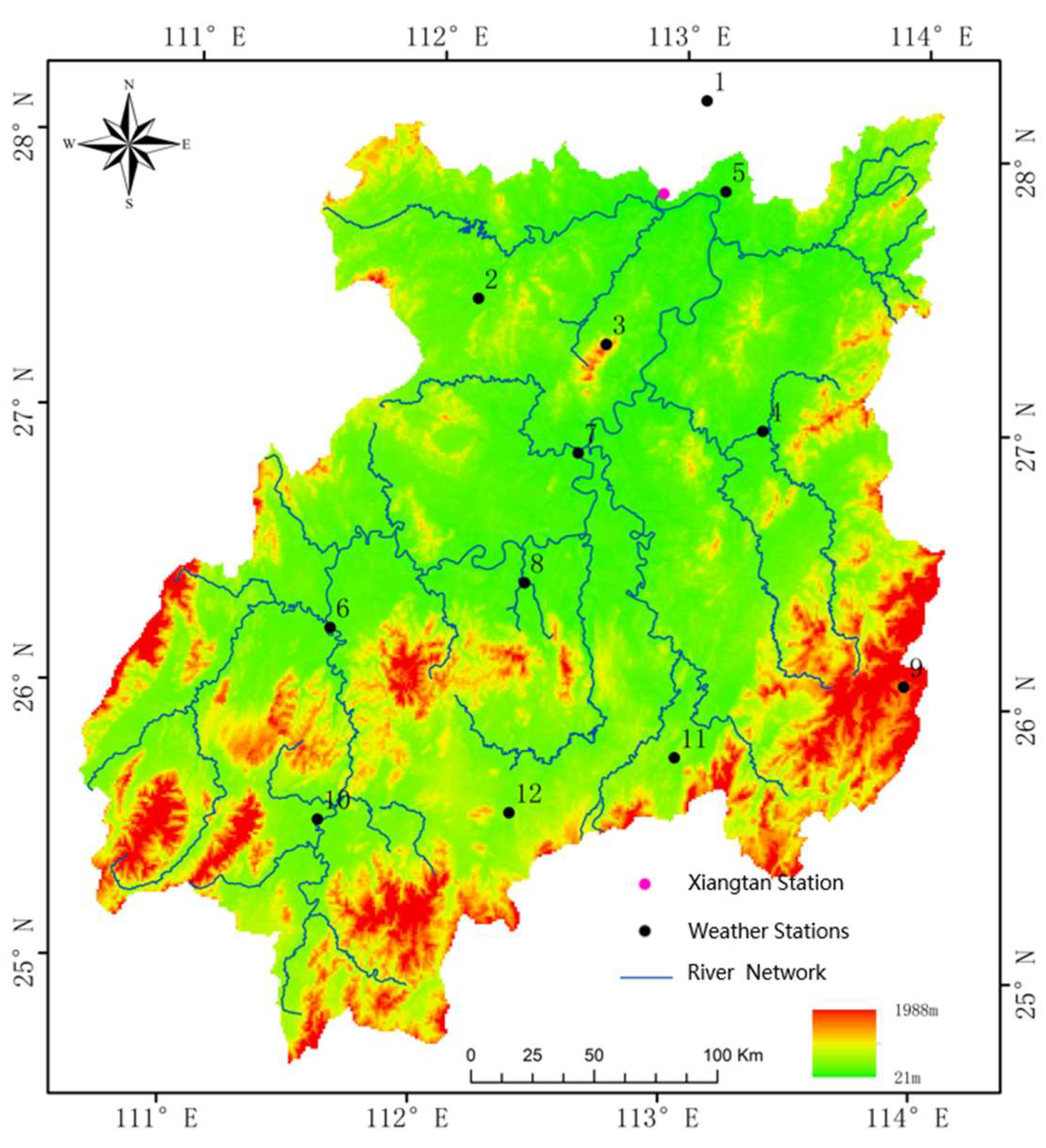
2. Study Area and Data

This study evaluates the SMBC method in the Xiangjiang River Basin (Figure 1), highlighting the importance of spatial correlation for hydrological simulations in large watersheds. The basin, part of the Dongting River system in the Yangtze River Basin, spans 884 km with a drainage area of 81,600 km² and lies in a subtropical humid region. Annual precipitation ranges from 1200 to 1700 mm, with over 45% occurring between April and June.

We used observed meteorological data (1960–2005) from 12 stations, including daily precipitation, maximum temperature, and minimum temperature, sourced from the China Meteorological Data Network (http://data.cma.cn/, assessed on 16 December 2023). Streamflow data from the Xiangtan station at the basin outlet were also used for model calibration. Simulated data were derived from 10 GCMs in the International Coupled Model Intercomparison Project Phase 5 (CMIP5), as detailed in Liu et al. [42]. The inverse distance weighting method was applied to generate station-level daily data from the four nearest grid points for each station.

3. Methodology

3.1. Bias Correction Method

This study proposes the SMBC method, which integrates the DBC method, Markov chains, and the distribution-free shuffle algorithm. This approach effectively leverages the strengths of the DBC method in correcting variable distributions, the Markov chains in correcting precipitation temporal sequences, and the shuffle algorithm in simulating spatial correlations. Before introducing the SMBC method, this section first introduces the core components of the above methods.

3.1.1. Simulating of Distribution

This study uses the DBC method [43] to correct the distribution characteristics of climate variables. The DBC method is a combination of the Daily Translation (DT) method [44] and the Local Intensity Scaling (LOCI) method [45]. After correcting the precipitation occurrence frequency using the DT method, the LOCI method is applied to calibrate the empirical distribution of variables. As a variant of the QM method, DBC is widely used in climate change research due to its simplicity and effectiveness [3,46,47]. The steps for the DBC method are as follows:

(1)

For each month, a threshold is set for the precipitation series simulated by the climate model to ensure that the wet-day frequency in the simulation in the historical period matches that of the observation. This threshold is then applied to precipitation series of simulations in the future period to determine the weather state.

(2)

The bias of the simulated series relative to the observation in terms of the empirical distribution represented by the 1st to 100th percentiles during the historical period is calculated as the correction factor. The same bias is removed from the empirical distribution of precipitation and temperature in the future. The calculation formula for correcting simulated precipitation is as follows:

$$P_{cor,his,m,p}=\left({\displaystyle \frac{P_{obs,m,p}}{P_{his,m,p}}}\right)\cdot P_{his,m,p}$$

(1)

$$P_{cor,fut,m,p}=\left({\displaystyle \frac{P_{obs,m,p}}{P_{his,m,p}}}\right)\cdot P_{fut,m,p}$$

(2)

P_his and P_fut represent simulated precipitation in historical and future periods; P_obs represents observed precipitation, m represents month, cor represents corrected, and p represents percentile. For temperature, the calculation of correction factors involves addition and subtraction.

3.1.2. Simulation of Precipitation Occurrence

Applying the first-order two-state Markov chain to simulate the precipitation sequence involves two parameters: the precipitation transition probabilities P₀₁ and P₁₁. Here, “1” represents wet days, and “0” represents dry days. P₀₁/P₁₁ represents the precipitation probabilities on the following day if the previous day is a dry/wet day. Given the weather state of the previous day, for example, a dry day, a uniformly distributed random number between 0 and 1 is first generated. A wet day is generated if this number exceeds P₀₁. Otherwise, a dry day is generated.

The downscaling of precipitation occurrence involves the adjustment of the above two transition probabilities of precipitation (P₀₁ and P₁₁). Previous studies [48,49,50] have shown a robust linear relationship between the precipitation transition probabilities and the mean monthly precipitation. Once a linear relationship is established using observed precipitation, the precipitation transition probabilities for that period can be obtained using the linear relationship and the downscaled mean monthly precipitation. Therefore, the key to using first-order two-state Markov chains for simulating precipitation lies in accurately downscaling the mean monthly precipitation, and the DBC method can effectively achieve this goal.

3.1.3. Simulation of Spatial Correlation

Imman and Conver [51] proposed the distribution-free shuffle algorithm to construct the correlation of independent variables without disturbing marginal distribution. The principle of this method is the following: assuming that [C] is the target correlation matrix, which is a positive definite symmetric matrix, it can be decomposed into the product of the lower triangular matrix and the corresponding transpose through Cholesky decomposition; that is, [C] = [P] [P’]. For any matrix of the same order [X], the correlation matrix of the matrix [D] ([D] = [X] [P’]) obtained by multiplying it with [P’] is also [C]. Take the simulation of the spatial correlation of precipitation occurrence as an example:

(1)

Calculate the n × n spatial correlation matrix [C] for precipitation occurrence, where n represents the number of stations. To ensure the matrix is positive definite, set any elements in its eigenvalue vector that are less than 0 to 0.0001, then recompose these eigenvalues into the correlation matrix [C].

(2)

Perform Cholesky decomposition on [C], resulting in [C] = [P][P’], where [P] is a lower triangular matrix and [P’] is its transpose. For any random matrix [X] multiplied by [P], the resulting matrix [D] will exhibit the same spatial correlation structure as [C].

(3)

The spatially correlated random number matrix [D], together with the simulated precipitation transition probability parameters, is used to generate a precipitation occurrence sequence with spatial correlation.

According to this principle, the distribution-free shuffle method can establish correlations between variables and spatial correlations with the same variable. When establishing the spatial correlation matrix of precipitation, the distribution-free method involves multiplying the decomposed matrix of the observed spatial correlation by a matrix of random numbers (for precipitation occurrence, the random number generated from the Markov chain). This multiplication yields simulated precipitation with spatial correlation while maintaining the desired marginal distributions of the variables.

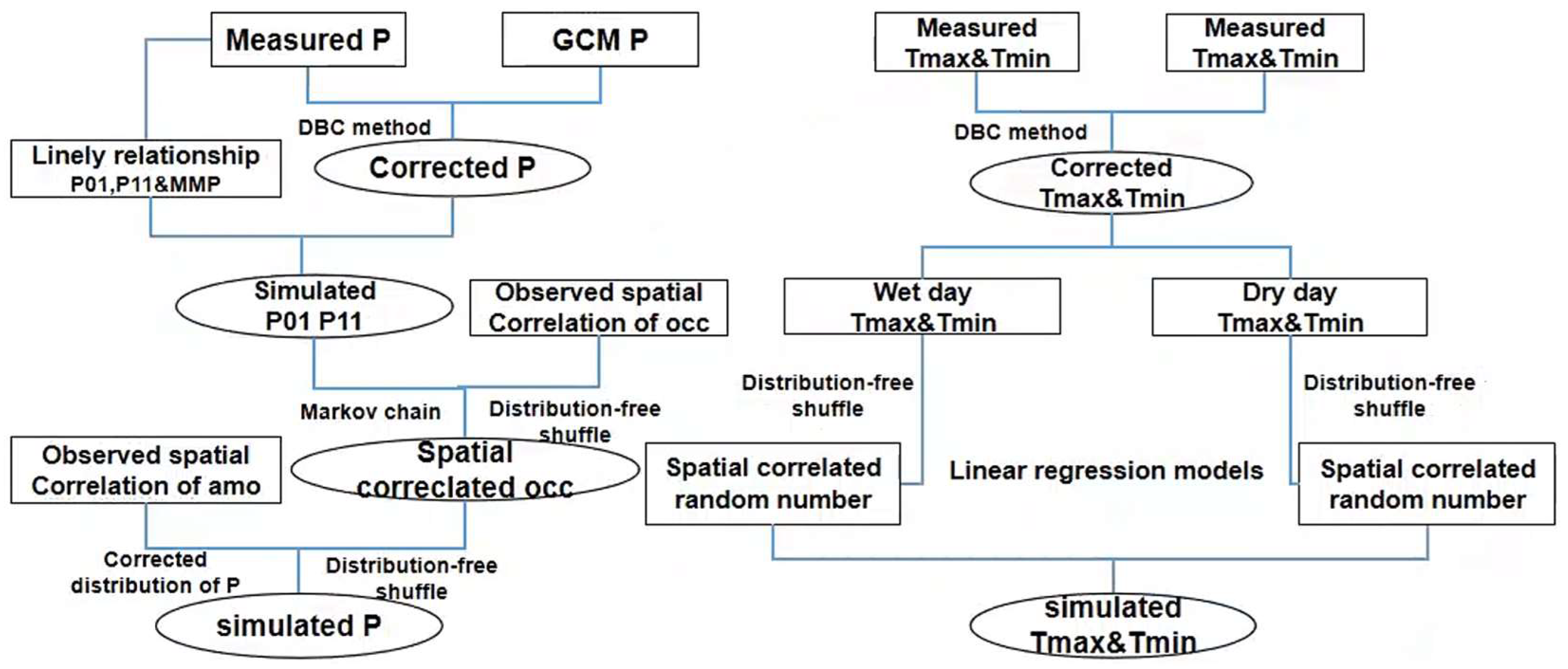
3.1.4. The Stochastic Multisite Bias Correction Method

Based on the above three core steps, the specific process of the SMBC method is as follows:

(1)

According to the four-point regression method [50], the linear relationship between the precipitation transition probabilities and the mean monthly precipitation is constructed monthly.

(2)

The DBC method is employed to correct the distributions of precipitation and temperature, from which the corrected mean monthly precipitation is obtained.

(3)

Spatial correlation matrices for observations (precipitation amount, precipitation occurrence, maximum temperature, minimum temperature) are calculated every month. By employing the distribution-free shuffle algorithm, the Cholesky decomposition is performed on these spatial correlation matrices. Multiply the decomposed lower triangular matrices by random number matrices, resulting in random number matrices that maintain the same spatial correlation as the observation.

(4)

Using the downscaled precipitation transition probabilities from step (2) and the spatially correlated random number matrix of precipitation occurrence in step (3), the first-order two-state Markov chain is employed to simulate the precipitation occurrence at each station.

(5)

The spatial correlation matrix of the precipitation amount from step (3) is normalized and multiplied by the spatially correlated random number matrix of the precipitation occurrence, yielding a spatial correlation matrix for the wet-day precipitation amount. The generated wet-day precipitation amounts are sampled from the corrected precipitation of the DBC method, according to the random number ranks in the correlation matrix. Finally, an overall scaling procedure is applied to ensure the water balance of the monthly total precipitation amount.

(6)

The temperature series are divided into wet-day maximum temperature/minimum temperature and dry-day maximum temperature/minimum temperature. Based on this categorization, a regression model for temperature is established. The spatially correlated random numbers computed in step (3) are input into the linear regression model to generate the temperature series.

The methodological framework of the SMBC method is show in Figure 2. Theoretically, the distribution-free shuffle algorithm introduces the observed spatial correlation matrix of variables into the random number matrix, thereby ensuring that the simulated spatial correlations of variables are consistent with the observed values. However, in practice, the rank correlations of the matrix obtained from the above steps are lower than expected [49,52]. Hence, based on the difference in spatial correlation between the generated data and the observed data, an additive iteration is applied to the spatially correlated random number matrix until the spatial correlation difference between the simulated data and the observed data is less than 0.01.

3.2. Hydrological Modeling

Hydrological simulations were conducted using the Soil and Water Assessment Tool (SWAT), a semi-distributed hydrologic model developed by the USDA Agricultural Research Center [53]. SWAT is a continuous, watershed-scale model with robust hydro-physical mechanisms capable of simulating hydrological processes and water balance dynamics. The model structure comprises four key modules: evapotranspiration, surface runoff, groundwater flow, and watershed routing. The study area is divided into multiple sub-basins, which are further subdivided into hydrological response units (HRUs)—regions within the same sub-basins sharing common attributes such as soil type, land use, and slope.

SWAT employs the Penman formula to estimate potential evapotranspiration, the Soil Conservation Service (SCS) runoff curve method to calculate surface runoff, and the Muskingum routing algorithm to simulate watershed routing processes. Model inputs include a digital elevation model and soil properties.

Model input data includes the digital elevation model (DEM), soil property information, land use data, watershed slope data, and meteorological and hydrological data, among others. The daily meteorological series, comprising precipitation and temperature data, are directly used to drive the SWAT model. Other meteorological variables (e.g., evapotranspiration, relative humidity, solar radiation, and wind speed) are generated by the model’s built-in stochastic weather generator. Model calibration and validation were conducted using data from 1960 to 1982 and 1983 to 2005, respectively. SWATCUP (the SWAT official calibration tool), SUFI2 (the optimization algorithm), and the Nash-Sutcliffe efficiency coefficient (NSE) were employed for calibration. The resulting NSE values were 0.873 and 0.785 for the two periods, respectively. Streamflow prediction errors (RE) were −6.05% and 1.9%, indicating good performance of the SWAT model in simulating the Xiangjiang River Basin (Figure 3).

3.3. Data Analysis

In the validation process, traditional methods divide data into calibration and validation periods chronologically. However, interannual variability may influence results. In this study, odd- and even-year datasets are alternately designated as calibration and validation periods, forming 46 complete validation datasets. To eliminate hydrological model bias, streamflow simulated by a meteorological model is used instead of measured streamflow. Based on the Indicators of Hydrological Alteration (IHA), hydrological environmental flow component parameters, and the research of Su [3], the performance of the two bias correction methods in reproducing 12 hydrological indicators are expounded, with specific indicators listed in

Table 1. Indices for evaluating the performance of bias correction methods on streamflow simulation.

Mean Value Index ID	Description
1	Annual mean flow (m3/s)
2	Mean flow in the rainy season (Apr. to Jul.) (m3/s)
Extreme Value Index ID	Description
3	Ten-year return period streamflow (m3/s)
4	Twenty-year return period streamflow (m3/s)
5	Fifty-year return period streamflow (m3/s)
6	Hundred-year return period streamflow (m3/s)
7	Annual maximum flow of one day (m3/s)
8	Annual maximum flow in intervals of consecutive three days (m3/s)
9	Annual maximum flow in intervals of five consecutive days (m3/s)
10	Annual flow of 90th quantile (m3/s)
11	Annual flow of 95th quantile (m3/s)
12	An extreme streamflow process is the consecutive days when QN > Q90 (day)
13	Number of extreme streamflow processes (times)
14	Total streamflow of extreme streamflow processes (m3)

.

The results mainly include the meteorological correction and corresponding hydrological simulations. In the meteorological correction section, the performance of the GCMs and two bias correction methods is demonstrated in terms of multiple spatial correlation metrics, such as simulated wet-day frequency, precipitation amount, and temperature. Meanwhile, the capabilities of the two bias correction methods in correcting precipitation distribution attributes are evaluated. In the hydrological simulation assessment, the performance of bias-corrected data in simulating monthly streamflow processes, extreme indicators, and mean value indicators is described.

4. Results

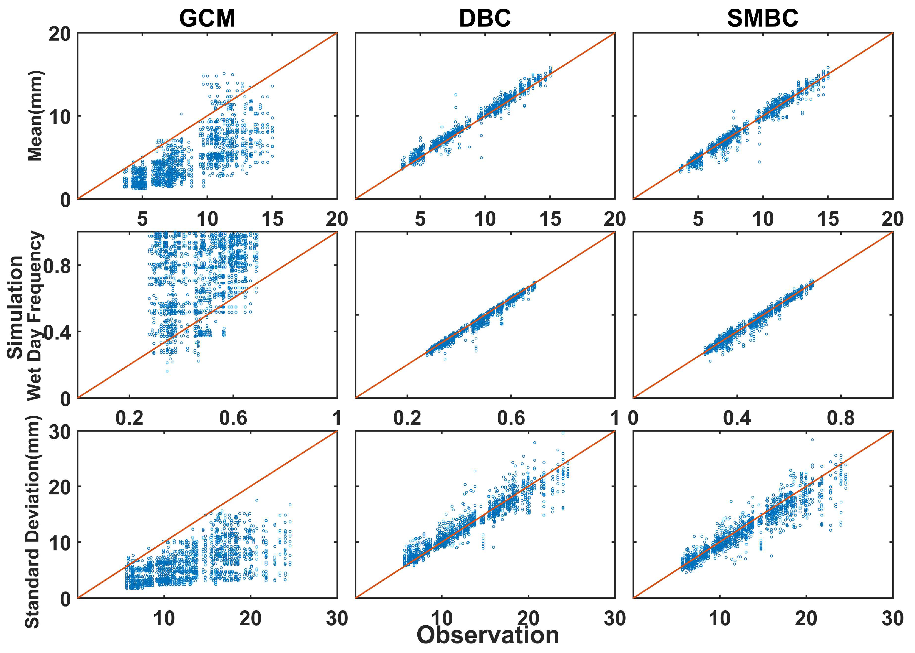
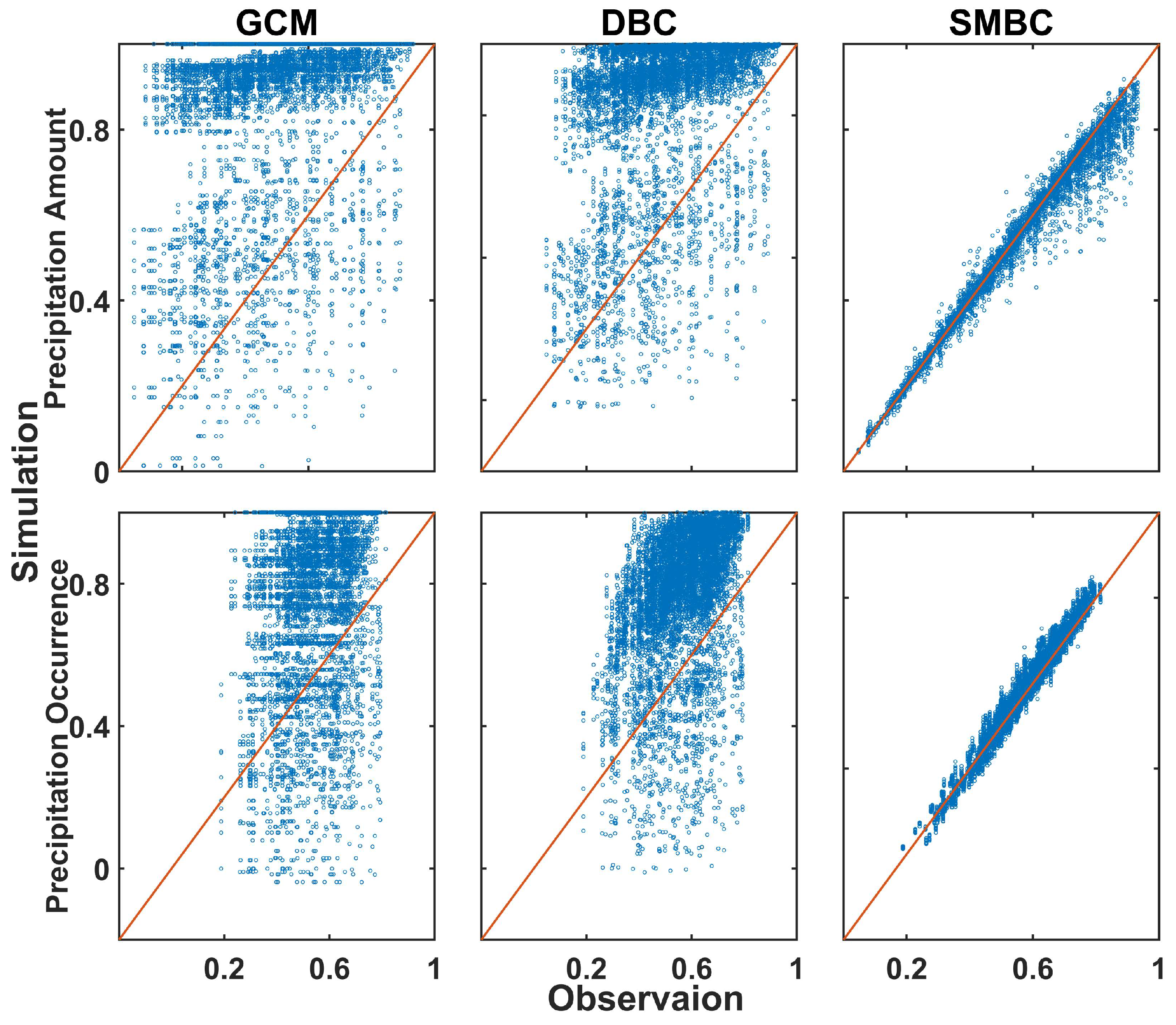
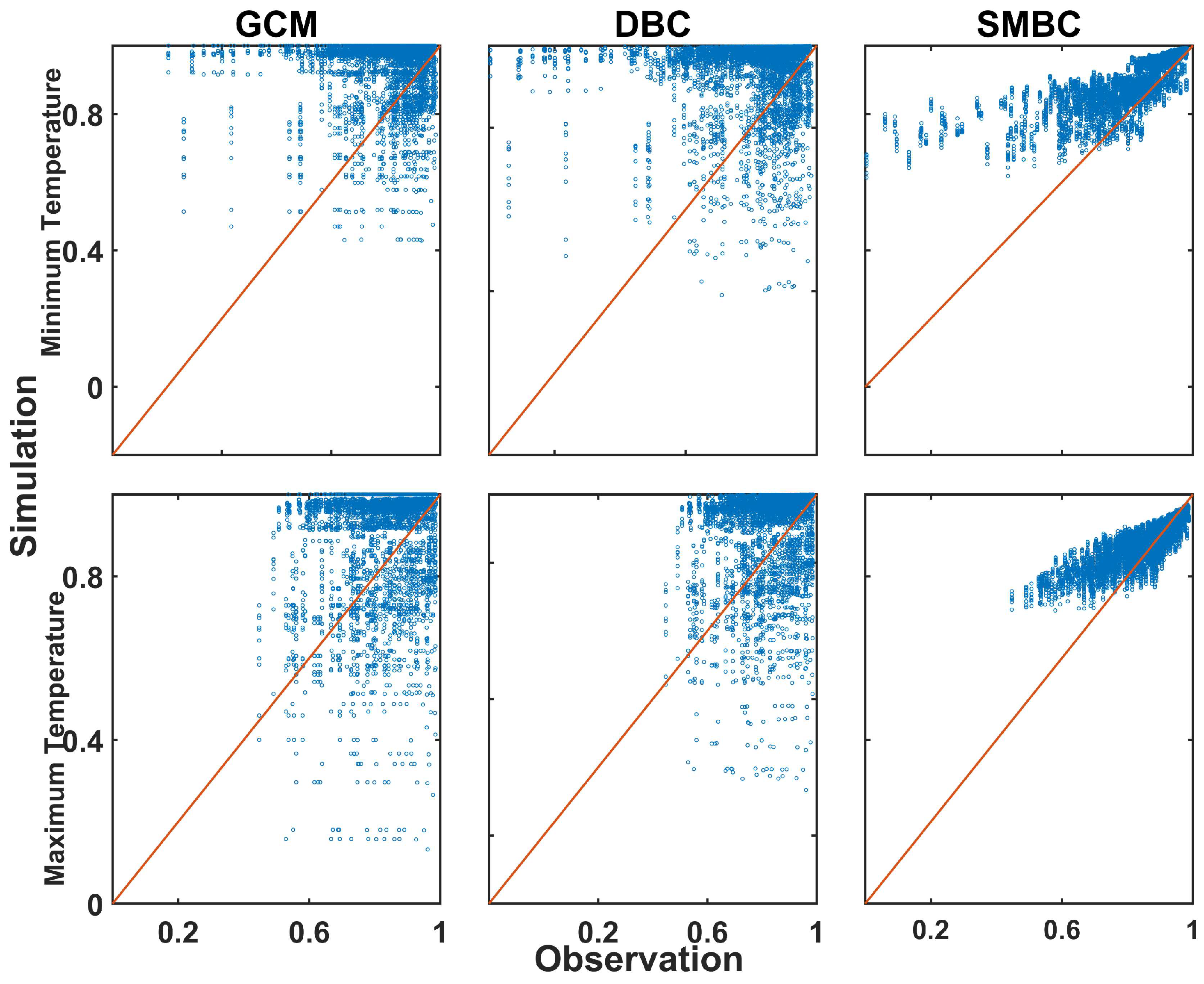
4.1. SMBC and DBC in Meteorological Correction

Figure 4 shows the mean, standard deviation of daily precipitation, and the wet-day frequency for each month at stations simulated by the GCMs and corrected by two bias correction methods. The mean absolute error (MAE) of these simulated indexes is shown in

Table 2. The MAE of the GCMs simulated and bias-corrected the mean, wet-day frequency, and standard deviation of daily precipitation at stations each month.

The Number of GCMs	Mean Daily Precipitation (mm)			Wet-Day Frequency			Standard Deviation (mm)
	GCM	DBC	SMBC	GCM	DBC	SMBC	GCM	DBC	SMBC
M1	2.56	0.26	0.21	0.42	0.01	0.01	4.99	0.91	1.02
M2	4.9	0.26	0.37	0.44	0.01	0.01	9.36	1.07	1.94
M3	3.6	0.27	0.2	0.21	0.01	0.01	6.24	0.77	0.95
M4	3.97	0.31	0.37	0.22	0.02	0.02	7.04	0.8	0.98
M5	5.51	0.29	0.43	0.36	0.01	0.02	9.41	0.96	1.8
M6	4.91	0.52	0.56	0.23	0.02	0.02	8.19	1.58	1.55
M7	4.59	0.5	0.41	0.24	0.02	0.01	7.59	1.57	1.24
M8	2.3	0.24	0.22	0.32	0.01	0.01	4.46	0.76	1.08
M9	2.7	0.44	0.27	0.15	0.02	0.01	5.48	0.81	0.86
M10	2.58	0.46	0.26	0.15	0.02	0.01	5.04	1.06	1.11

. The results show that all GCMs predict too much drizzle, thus underestimating precipitation intensity and standard deviation. The MAE of the wet-day frequency for each month simulated by the GCMs ranges from 0.15 to 0.45, while the mean precipitation ranges from 2.30 mm to 5.51 mm, and the standard deviation is between 4.46 mm and 9.41 mm. Both bias correction methods effectively correct the mean, the wet-day frequency, and the standard deviation of precipitation. Corrected by the DBC method, the MAE of the wet-day frequency ranges from 0.01 to 0.02, and the mean and standard deviation range from 0.24 mm to 0.52 mm and from 0.76 mm to 1.58 mm, respectively. The SMBC method introduces slightly larger biases due to its use of two additional stochastic processes. These biases may improve with longer data lengths or when inter-annual metrics are calculated. The MAE of the simulated mean daily precipitation for each month ranges from 0.26 mm to 0.65 mm, from 0.90 mm to 1.91 mm for the standard deviation, and is around 0.01 for the wet-day frequency.

Figure 5 displays the correlations of daily precipitation amount between stations for each month simulated by the GCMs and corrected using two bias correction methods. The correlations of precipitation occurrence are also shown in Figure 4. GCM simulations are extracted by inverse distance weighting from the nearest four grids. Thus, its spatial correlations are higher than that of observation. Furthermore, GCM simulations overestimate drizzle, leading to an overestimation of spatial correlations of precipitation occurrence. The simulated spatial correlation coefficients of precipitation occurrence generally exceed 0.8, whereas the observation ranges from 0.2 to 0.8. The MAE of the two indicators simulated by GCMs and corrected using two bias correction methods are shown in

Table 3. MAE of spatial correlation coefficients of precipitation occurrence and amount between stations for each month simulated by GCMs and two bias correction methods.

The Number of GCMs	Precipitation Occurrence			Precipitation Amount
	GCM	DBC	SMBC	GCM	DBC	SMBC
M1	0.37	0.34	0.01	0.27	0.22	0.02
M2	0.39	0.38	0.01	0.38	0.29	0.02
M3	0.38	0.36	0.01	0.32	0.25	0.02
M4	0.38	0.36	0.02	0.32	0.26	0.02
M5	0.36	0.34	0.01	0.25	0.22	0.02
M6	0.38	0.36	0.02	0.33	0.26	0.01
M7	0.38	0.36	0.02	0.33	0.25	0.02
M8	0.38	0.35	0.02	0.27	0.23	0.02
M9	0.39	0.37	0.01	0.32	0.26	0.02
M10	0.39	0.37	0.01	0.33	0.26	0.02

, respectively. The MAE of the spatial correlation coefficients for GCM simulation of precipitation amounts ranges from 0.36 to 0.39, while those for precipitation occurrence range from 0.25 to 0.38. Significant bias in the spatial correlations of precipitation amount and occurrence persists even after applying the DBC method. The SMBC method substantially reduces the biased output of the GCMs. The MAE of the spatial correlation coefficients for simulated precipitation occurrence range from 0.01 to 0.02, while for precipitation amount they are within 0.02.

Figure 6 illustrates spatial correlations of daily maximum and minimum temperatures between stations for each month, as simulated by the GCMs and corrected using two bias correction methods. Realistic correlation coefficients exceed 0.4, often surpassing 0.6, reflecting stronger temperature spatial correlations than precipitation. The MAE of these correlations, as simulated by the GCMs and corrected using two methods, is shown in

Table 4. As for Table 3, but for the maximum temperature and minimum temperature.

The Number of GCMs	Maximum Temperature			Minimum Temperature
	GCM	DBC	SMBC	GCM	DBC	SMBC
M1	0.12	0.12	0.05	0.16	0.15	0.09
M2	0.17	0.17	0.05	0.18	0.18	0.09
M3	0.13	0.12	0.05	0.16	0.16	0.08
M4	0.13	0.12	0.05	0.16	0.15	0.08
M5	0.12	0.12	0.05	0.15	0.14	0.08
M6	0.13	0.12	0.05	0.16	0.15	0.08
M7	0.13	0.12	0.05	0.16	0.15	0.08
M8	0.12	0.12	0.05	0.15	0.15	0.08
M9	0.12	0.11	0.05	0.15	0.15	0.08
M10	0.12	0.11	0.05	0.15	0.15	0.09

. For daily maximum temperature, the MAE ranges from 0.12 to 0.17. For the minimum temperature, it ranges between 0.15 and 0.18. After DBC correction, the MAE of the daily maximum temperature correlation coefficients ranges from 0.11 to 0.17, and for minimum temperature it is also similar. The SMBC method outperforms the DBC method for both the spatial correlation of daily maximum and maximum temperature, although it is slightly overestimated.

Further investigation into modeling spatial correlation of weather states is presented in Figure 7, which evaluates the performance of the GCMs and two bias-correction methods in simulating the probabilities of two stations experiencing wet or dry days simultaneously. The MAE relative to observation is shown in

Table 5. The MAE of the GCMs simulated and the bias correction method corrected the probability of two stations having wet days/dry days simultaneously.

	Wet Days			Dry days
	GCM	DBC	SMBC	GCM	DBC	SMBC
M1	0.51	0.04	0.01	0.34	0.06	0.01
M2	0.52	0.07	0.01	0.35	0.07	0.01
M3	0.28	0.05	0.01	0.14	0.06	0.01
M4	0.27	0.05	0.02	0.17	0.07	0.02
M5	0.43	0.05	0.02	0.28	0.06	0.02
M6	0.27	0.05	0.02	0.2	0.08	0.03
M7	0.3	0.05	0.01	0.19	0.07	0.01
M8	0.41	0.05	0.01	0.24	0.06	0.01
M9	0.21	0.05	0.01	0.11	0.08	0.01
M10	0.21	0.05	0.01	0.11	0.08	0.01

. The GCMs significantly overestimate the wet-day frequency, resulting in overestimating the probabilities of two stations experiencing wet days simultaneously, with MAE up to 0.52. Conversely, the occurrence of two stations experiencing dry days simultaneously is less frequent, with probabilities underestimated (MAE between 0.11 and 0.35). The DBC method improves the simulation of these probabilities by correcting wet-day frequency, with MAE ranging from 0.04 to 0.07 for wet days and from 0.06 to 0.08 for dry days. This suggests that the GCMs can simulate precipitation at individual stations if drizzle events are excluded. The SMBC method also reproduces this phenomenon, with scatter plots showing a more even distribution around the 1:1 line post correction. The MAE of SMBC-corrected probabilities for two stations having wet days simultaneously ranges from 0.01 to 0.02, while for dry days, it ranges from 0.01 to 0.03.

Spatial correlation may have a more significant impact on watershed-scale meteorological and hydrological simulations. Figure 8 shows the quantile/quantile plot of the mean, standard deviation, and wet-day frequency of watershed-averaged monthly precipitation series simulated by the GCMs and corrected by the two bias correction methods, respectively. The GCMs underestimate the mean and standard deviation of precipitation and overestimate the wet-day frequency. The DBC method eliminates most bias in simulating precipitation but underestimates the wet-day frequency and overestimates the standard deviation. The SMBC method outperforms the DBC method in simulating the mean precipitation and more accurately captures the standard deviation and wet-day frequency of the precipitation series due to its consideration of variable spatial correlation.

Figure 9 illustrates the absolute relative error (ARE) of the mean annual maximum accumulated precipitation over 1-, 3-, and 5-day periods simulated by the GCMs and corrected by the two bias correction methods. The GCMs overestimate the mean annual maximum accumulated precipitation over these time scales, with ARE ranging from 1.1% to 57.9%, 3.2% to 50.2%, and 2.1% to 47.2%, respectively. The DBC method exhibits the largest bias magnitudes in these extreme precipitation events, likely due to the inverse distance weighting interpolation of the GCM grid data, which results in a consistent precipitation state and magnitude among neighboring stations within the basin. This causes excessive simulation of extreme precipitation events, as noted in previous studies by Maraun [6]. In contrast, the SMBC method performs better in reproducing the observed mean annual maximum accumulated precipitation over 1-, 3-, and 5-day periods, with the ARE ranging from 0.9% to 16.1%, 4.7% to 15.6%, and 4.4% to 16.5%, respectively.

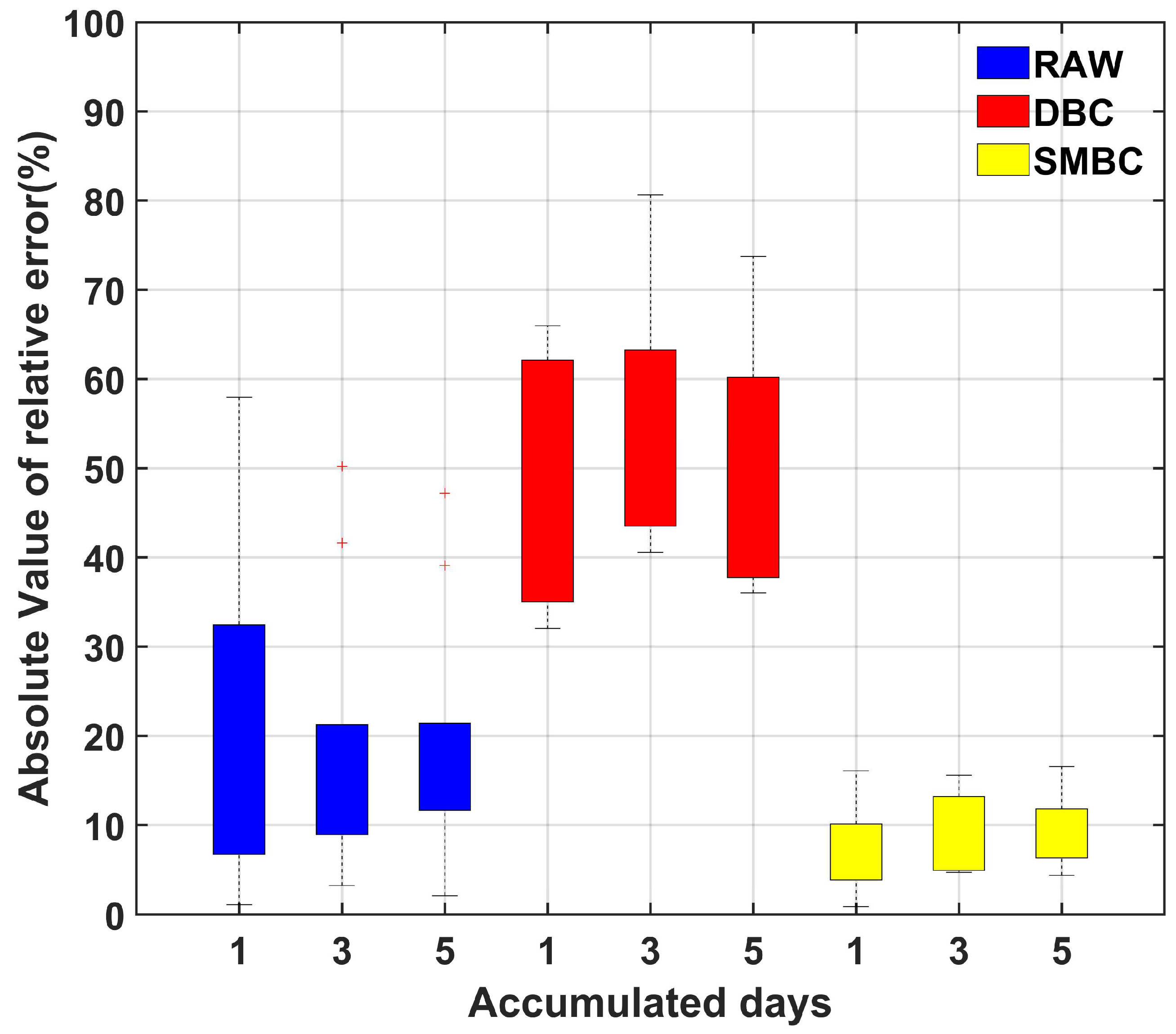
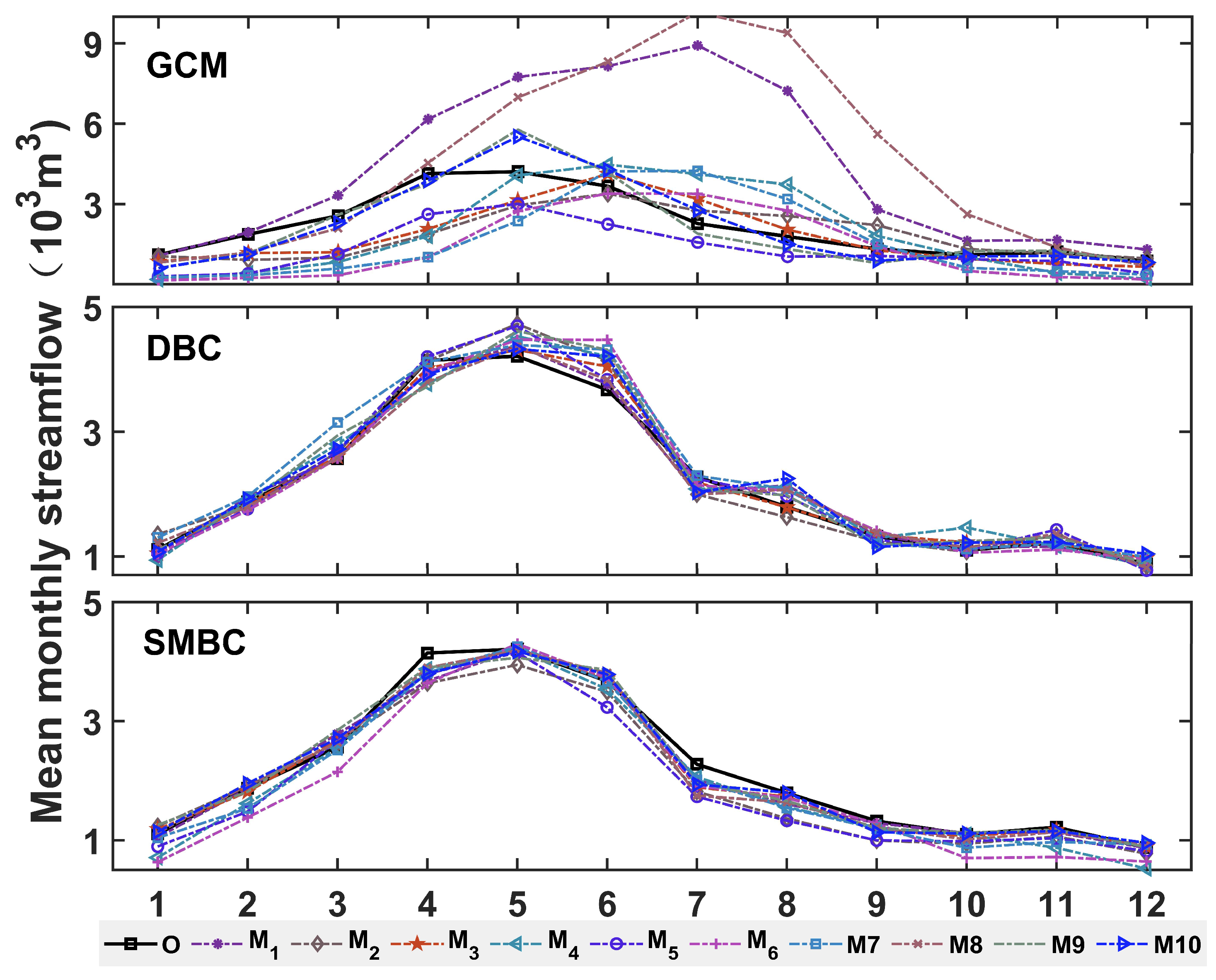
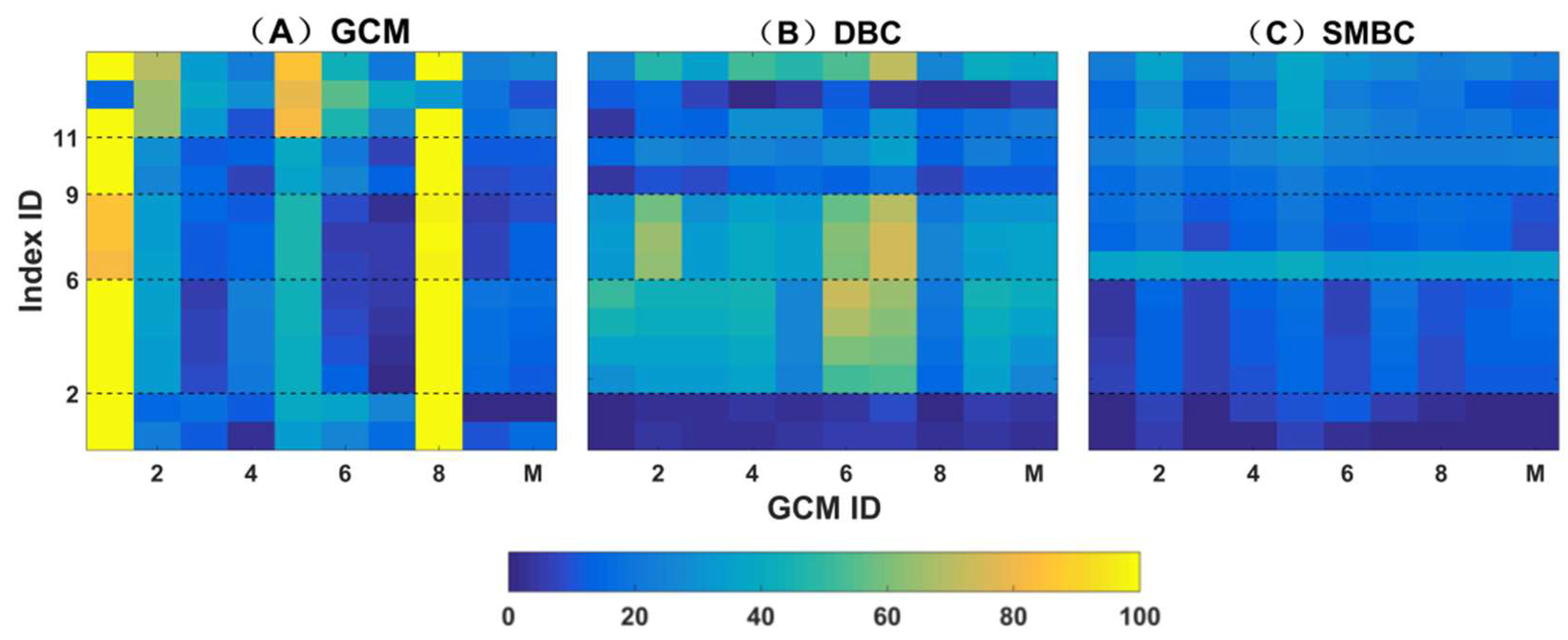
4.2. SMBC and DBC in Hydrological Simulation

Daily precipitation and temperature simulated by the GCMs and corrected by the two bias correction methods are used to drive the SWAT for hydrological simulation. Figure 10 shows the corresponding mean monthly streamflow process. By hydrological simulation, the outputs of the GCMs can roughly reproduce the intra-annual distribution of observed streamflow. However, the overall biases are extensive, with the RE of the simulated mean monthly streamflow exceeding 100% in most of the months for M2 and M8 (the GCM no.). The DBC method significantly reduces these biases, though there remains a slight overestimation of the overall process, especially in May, June, and August. The meteorological data corrected by the SMBC method also reproduces the intra-annual distribution of streamflow well, with an overall improvement in mean monthly streamflow. However, there is also a slight underestimation. Both bias correction methods reduce the uncertainty of GCM output in simulating streamflow.

To further explore the differences between the two bias correction methods in the hydrology simulation, Figure 11 shows the performance of the data corrected by the two bias correction methods in simulating mean and extreme streamflow indicators, along with GCM simulation results. The y-axis represents the ARE of the two bias correction methods and the GCM simulation in reproducing fourteen statistics concerning streamflow (in Table 1), with the y-axis coordinate corresponding to the specific indicator number. The simulated streamflow based on GCM outputs exhibits significant bias in mean value indicators. Specifically, the ARE of the mean daily streamflow and mean daily streamflow during the rainy season ranges from 10.5% to 107.0% and 11.1% to 119.9%, respectively. Both bias correction methods effectively reduce the bias. The ARE of the mean daily streamflow simulated by the DBC method correction ranges from 0.51% to 8.1%, and the mean daily streamflow in the rainy season ranges from 0.9% to 5.1%. Consistent with the findings for mean monthly streamflow, the mean values of daily and rainy season streamflow simulated by the SMBC method are smaller than those by the DBC method. However, the magnitude of the biases remains consistent with the DBC method. Additionally, both methods successfully reduce simulation uncertainty.

For extreme streamflow simulation, the ARE of the return period streamflow indicators (No. 3–6) simulated by GCM outputs ranges from 0.1% to 115.9% with notable uncertainty. After applying the DBC method, the range of ARE for these indicators is reduced from 15.3% to 73.3%, with a mean ARE of 39.9%, which is more significant than the GCM simulations. These findings are consistent with precipitation simulation results. While the DBC method corrects the spatial distribution of precipitation at stations, the excessive spatial correlation leads to an overestimation of extreme precipitation and, consequently, an overestimation of extreme streamflow. For other extreme streamflow indicators (e.g., indices 7–9 for maximum runoff over 1-, 3-, and 7-day periods; indices 10–11 for the 90th and 95th percentiles of streamflow; and the number of extreme flooding days, events, and total streamflow), the simulation performance of GCM outputs and the two bias correction methods is comparable to that of return period streamflow indicators. Specifically, the indicators simulated by GCM outputs exhibit significant biases. The DBC method either reduces or amplifies these biases, while the SMBC method significantly reduces biases for extreme events. Furthermore, both the DBC and SMBC methods effectively reduce the uncertainty in GCM simulations.

5. Summary

Bias correction methods have become a standard procedure for linking climate model outputs with impact models [38,54]. However, most bias correction methods are applied independently at stations, neglecting the spatial correlation of variables [7,55]. Therefore, this study proposes the SMBC method and validates its performance over the Xiangjiang River Basin.

The results indicate that the GCMs overestimate drizzle and spatial correlation of precipitation amount and precipitation occurrence. The GCMs overestimate the probability of two stations experiencing wet days simultaneously, while dry days are underestimated. Both bias correction methods effectively reduce the distribution biases at the station scale. The DBC method performs well in correcting the wet-day frequency and precipitation distribution, achieving good performance in simulating the probability of two stations experiencing wet days simultaneously. However, as it neglects the spatial correlation attributes of precipitation and temperature, it replicates the GCMs’ biases in spatial correlation, leading to significant errors in watershed-averaged precipitation distribution. The SMBC method effectively reproduces the spatial correlation of the precipitation amount, precipitation occurrence, and temperature. It also significantly improves the GCMs’ simulation of the probabilities of two stations experiencing wet/dry days simultaneously, accurately reproducing variable distributions in watersheds. Hydrological simulation shows that bias-corrected data using both methods reproduce mean streamflow processes, including monthly and daily averages. Additionally, SMBC demonstrates clear advantages in replicating extreme streamflow processes, such as return period flows and multi-day accumulated flows.

The advantages of the SMBC method are as follows: (1) The distribution-free shuffle algorithm is incorporated to account for the stochastic nature of precipitation occurrence and amounts, introducing randomness to avoid potential inflation issues, as Maraun [6] recommended. (2) Although the three steps are interconnected, they are relatively independent and flexible. For instance, the DBC method can be substituted with other bias correction methods that effectively correct variable distributions. Additionally, the distribution-free shuffle algorithm can be replaced with alternative functions that maintain the marginal distributions of variables while introducing spatial correlation matrices. (3) The SMBC method effectively corrects the distribution of variables, precipitation occurrence, and their spatial correlations, thereby improving hydrological simulation accuracy. This study primarily provides a framework for bias correction.

However, no correction method can comprehensively address all the biases present in GCM outputs. The limitations of the SMBC method are as follows: (1) The SMBC method focuses on building spatial correlation of variables without considering the correlation between variables, which is also significant for hydro-meteorological research [9,36]. Therefore, future research could use a shuffle algorithm to establish the correlation between variables again. (2) Similar to most bias correction methods, the SMBC method also follows the assumption of stationarity. Ignoring the nonstationarity of climate change leads to more bias in the model validation period than in the calibration period, which affects the reliability of subsequent simulations. For example, Van et al. [56] explored the performance of univariate and multivariate bias correction methods under bias nonstationary. The results show that nonstationarity has a significant impact on the bias correction effects of all methods, especially when correcting winter and summer precipitation, a hidden danger for hydrological simulations. To address the issue of nonstationarity, future research can dig deeper into the key covariates affecting the nonstationary changes in spatial correlation (such as climate change indicators and terrain evolution factors) and establish a dynamic covariate-correlation structure response model to achieve real-time tracking and adaptive correction of nonstationarity [57].

The product of CMIP6 is more accurate in simulating atmospheric circulation, mean precipitation, and extreme precipitation compared to CMIP5, but there are still certain biases in its simulations [58,59,60,61]. Additionally, many studies have compared CMIP6 with CMIP5, and the results show that the simulation accuracy of CMIP6 is not comprehensively better than that of CMIP5. In some regions and seasons, CMIP5 performs better than CMIP6 [60,61]. Based on these two reasons and considering the continuity of the research [62], CMIP5 simulations are still used in this study to verify the effect of the bias correction method.

In summary, the SMBC method not only inherits the advantages of the DBC method in distribution correction but also integrates the spatial correlation of variables and temporal sequence of precipitation, featuring a clear conceptual framework and straightforward implementation steps. Compared with machine learning-based bias correction methods, the SMBC method has lower data requirements while effectively simulating extreme events. Its multiple correction capabilities position it as an ideal tool for hydrological impact studies of climate change in large watersheds. By providing more accurate bias-corrected climate input data, the SMBC method enhances the reliability of real-time flood forecasting, water resource management, and climate risk mitigation strategies, ultimately contributing to more resilient water infrastructure and sustainable environmental decision-making.

References

1. Ali, Z.; Hamed, M.M.; Muhammad, M.K.I.; Shahid, S. A novel approach for evaluation of CMIP6 GCMs in simulating temperature and precipitation extremes of Pakistan. Int. J. Clim. 2024, 44, 592–612. [Google Scholar] [CrossRef]
2. Iqbal, Z.; Shahid, S.; Ahmed, K.; Ismail, T.; Ziarh, G.F.; Chung, E.-S.; Wang, X. Evaluation of CIMP6 GCM rainfall in mainland Southeast Asia. Atmos. Res. 2021, 254, 105525. [Google Scholar] [CrossRef]
3. Su, T.; Chen, J.; Cannon, A.J.; Xie, P.; Guo, Q. Multi-site bias correction of climate model outputs for hydro-meteorological impact studies: An application over a watershed in China. Hydrol. Process. 2020, 34, 2575–2598. [Google Scholar] [CrossRef]
4. Goswami, P.; Saha, S.; Das, L.; Banerjee, S. Evaluation of CMIP6 GCMs performance and future projection for the Boro and Kharif seasons over the new alluvial zones of West Bengal. J. Agrometeorol. 2024, 26, 168–173. [Google Scholar] [CrossRef]
5. Lorenzo, M.; Meucci, A.; Liu, J.; Syktus, J.; Thatcher, M.; Young, I. From global to regional-scale CMIP6-derived wind wave extremes: A single-GCM HighResMIP and CORDEX downscaling experiment in South-East Australia. Clim. Dyn. 2025, 63, 97. [Google Scholar] [CrossRef]
6. Maraun, D. Bias Correction, Quantile Mapping, and Downscaling: Revisiting the Inflation Issue. J. Clim. 2013, 26, 2137–2143. [Google Scholar] [CrossRef]
7. Nahar, J.; Johnson, F.; Sharma, A. Addressing Spatial Dependence Bias in Climate Model Simulations: An Independent Component Analysis Approach. Water Resour. Res. 2018, 54, 827–841. [Google Scholar] [CrossRef]
8. Maraun, D.; Widmann, M.; Gutiérrez, J.M.; Kotlarski, S.; Chandler, R.E.; Hertig, E.; Wibig, J.; Huth, R.; Wilcke, R.A. VALUE: A framework to validate downscaling approaches for climate change studies. Earth’s Future 2014, 3, 1–14. [Google Scholar] [CrossRef]
9. Guo, Q.; Chen, J.; Zhang, X.; Shen, M.; Chen, H.; Guo, S. A new two-stage multivariate quantile mapping method for bias correcting climate model outputs. Clim. Dyn. 2019, 53, 3603–3623. [Google Scholar] [CrossRef]
10. Klein, W.H.; Glahn, H.R. Forecasting Local Weather by Means of Model Output Statistics. Bull. Am. Meteorol. Soc. 1974, 55, 1217–1227. [Google Scholar] [CrossRef]
11. Wilby, R.L.; Dawson, C.W.; Barrow, E.M. sdsm—A decision support tool for the assessment of regional climate change impacts. Environ. Model. Softw. 2002, 17, 145–157. [Google Scholar] [CrossRef]
12. Song, Y.H.; Chung, E.S.; Shahid, S. The New Bias Correction Method for Daily Extremes Precipitation over South Korea using CMIP6 GCMs. Water Resour. Manag. 2022, 36, 5977–5997. [Google Scholar] [CrossRef]
13. Amunugama, M.; Tanaka, Y.; Suzuyama, K.; Ogata, T. WRF Dynamical Downscaling for High-Intensity Typhoons of D4PDF. In Proceedings of the International Conference on Asian and Pacific Coasts, Kyoto, Japan, 14–17 November 2023; Springer: Singapore, 2024; pp. 243–253. [Google Scholar] [CrossRef]
14. Navarro-Racines, C.; Tarapues, J.; Thornton, P.; Jarvis, A.; Ramirez-Villegas, J. High-resolution and bias-corrected CMIP5 projections for climate change impact assessments. Sci. Data 2020, 7, 7. [Google Scholar] [CrossRef] [PubMed]
15. Doury, A.; Somot, S.; Gadat, S. On the suitability of a convolutional neural network based RCM-emulator for fine spatio-temporal precipitation. Clim. Dyn. 2024, 62, 8587–8613. [Google Scholar] [CrossRef]
16. Teutschbein, C.; Seibert, J. Bias correction of regional climate model simulations for hydrological climate-change impact studies: Review and evaluation of different methods. J. Hydrol. 2012, 456, 12–29. [Google Scholar] [CrossRef]
17. Jaiswal, R.; Mall, R.K.; Singh, N.; Kumar, T.V.L.; Niyogi, D. Evaluation of Bias Correction Methods for Regional Climate Models: Downscaled Rainfall Analysis Over Diverse Agroclimatic Zones of India. Earth Space Sci. 2022, 9, e2021EA001981. [Google Scholar] [CrossRef]
18. Xavier, A.C.F.; Martins, L.L.; Rudke, A.P.; de Morais, M.V.B.; Martins, J.A.; Blain, G.C. Evaluation of Quantile Delta Mapping as a bias-correction method in maximum rainfall dataset from downscaled models in So Paulo state (Brazil). Int. J. Climatol. 2022, 42, 175–190. [Google Scholar] [CrossRef]
19. Chen, J.; Arsenault, R.; Brissette, F.P.; Zhang, S. Climate Change Impact Studies: Should We Bias Correct Climate Model Outputs or Post-process Impact Model Outputs? Water Resour. Res. 2021, 57, e2020WR028638. [Google Scholar] [CrossRef]
20. Voropay, N.; Ryazanova, A.; Dyukarev, E. High-resolution bias-corrected precipitation data over South Siberia, Russia. Atmos. Res. 2021, 254, 105528. [Google Scholar] [CrossRef]
21. Maraun, D. Nonstationarities of regional climate model biases in European seasonal mean temperature and precipitation sums. Geophys. Res. Lett. 2012, 39, L06706. [Google Scholar] [CrossRef]
22. Chen, J.; Brissette, F.P.; Zhang, X.J.; Chen, H.; Guo, S.; Zhao, Y. Bias correcting climate model multi-member ensembles to assess climate change impacts on hydrology. Clim. Change 2019, 153, 361–377. [Google Scholar] [CrossRef]
23. Han, X.; Mehrotra, R.; Sharma, A. Measuring the spatial connectivity of extreme rainfall. J. Hydrol. 2020, 590, 125510. [Google Scholar] [CrossRef]
24. Li, X.; Vladan, B. A new scheme for multivariate, multisite weather generator with inter-variable, inter-site dependence and inter-annual variability based on empirical copula approach. Clim. Dyn. 2018, 52, 2247–2267. [Google Scholar] [CrossRef]
25. Yao, N.; Ye, J.; Wang, S.; Yang, S.; Lu, Y.; Zhang, H.; Yang, X. Bias correction of the hourly satellite precipitation product using machine learning methods enhanced with high-resolution WRF meteorological simulations. Atmos. Res. 2024, 310, 107637. [Google Scholar] [CrossRef]
26. Iqbal, Z.; Shahid, S.; Ahmed, K.; Wang, X.; Ismail, T.; Gabriel, H.F. Bias correction method of high-resolution satellite-based precipitation product for Peninsular Malaysia. Theor. Appl. Climatol. 2022, 148, 1429–1446. [Google Scholar] [CrossRef]
27. Meema, T.; Wattanasetpong, J.; Wichakul, S. Integrating machine learning and zoning-based techniques for bias correction in gridded precipitation data to improve hydrological estimation in the data-scarce region. J. Hydrol. 2025, 646, 132356. [Google Scholar] [CrossRef]
28. Pan, B.; Hsu, K.; AghaKouchak, A.; Sorooshian, S. Improving precipitation estimation using convolutional neural network. Water Resour. Res. 2019, 55, 2301–2321. [Google Scholar] [CrossRef]
29. Huang, B.; Liu, Z.; Duan, Q.; Rajib, A.; Yin, J. Unsupervised deep learning bias correction of CMIP6 global ensemble precipitation predictions with cycle generative adversarial network. Environ. Res. Lett. 2024, 19, 094003. [Google Scholar] [CrossRef]
30. Hu, Y.; Yin, F.; Zhang, W. Deep learning-based precipitation bias correction approach for Yin–He global spectral model. Meteorol. Appl. 2021, 28, e2032. [Google Scholar] [CrossRef]
31. Xu, L.; Chen, N.; Chen, Z.; Zhang, C.; Yu, H. Spatiotemporal forecasting in earth system science: Methods, uncertainties, predictability and future directions. Earth-Sci. Rev. 2021, 222, 103828. [Google Scholar] [CrossRef]
32. Ebert-Uphoff, I.; Hilburn, K. Evaluation, tuning and interpretation of neural networks for working with images in meteorological applications. Bull. Am. Meteorol. Soc. 2020, 101, E2149–E2170. [Google Scholar] [CrossRef]
33. Chen, J.; Chen, H.; Guo, S. Multisite precipitation downscaling using a stochastic weather generator. Clim. Dyn. 2018, 50, 1975–1992. [Google Scholar] [CrossRef]
34. Li, X.; Babovic, V. Multisite multivariate downscaling of global climate model outputs: An integrated framework combining quantile mapping, stochastic weather generator and Empirical Copula approaches. Clim. Dyn. 2018, 52, 5775–5799. [Google Scholar] [CrossRef]
35. Nguyen, V.D.; Merz, B.; Hundecha, Y.; Haberlandt, U.; Vorogushyn, S. Comprehensive evaluation of an improved large-scale multi-site weather generator for Germany. Int. J. Climatol. 2021, 41, 4933–4956. [Google Scholar] [CrossRef]
36. Wang, Y.; Xie, J.; You, Y.; Wang, Y.; Xu, Y.-P.; Guo, Y.-X. A new multisite multi-variable stochastic model with inter-site and inter-variable correlations, low-frequency attributes and stochasticity: A case study in the lower Yellow River basin. J. Hydrol. 2021, 599, 126365. [Google Scholar] [CrossRef]
37. Verdin, A.; Rajagopalan, B.; Kleiber, W.; Podestá, G.; Bert, F. A conditional stochastic weather generator for seasonal to multi-decadal simulations. J. Hydrol. 2018, 556, 835–846. [Google Scholar] [CrossRef]
38. Ben Alaya, M.A.; Chebana, F.; Ouarda, T.B.M.J. Multisite and multi-variable statistical downscaling using a Gaussian copula quantile regression model. Clim. Dyn. 2015, 47, 1383–1397. [Google Scholar] [CrossRef]
39. Hnilica, J.; Hanel, M.; Puš, V. Multisite bias correction of precipitation data from regional climate models. Int. J. Climatol. 2017, 37, 2934–2946. [Google Scholar] [CrossRef]
40. Franois, B.; Thao, S.; Vrac, M. Adjusting spatial dependence of climate model outputs with cycle-consistent adversarial networks. Clim. Dyn. 2021, 57, 3323–3353. [Google Scholar] [CrossRef]
41. François, B.; Vrac, M.; Cannon, A.J.; Robin, Y.; Allard, D. Multivariate bias corrections of climate simulations: Which benefits for which losses? Earth Syst. Dyn. 2020, 11, 537–562. [Google Scholar] [CrossRef]
42. Liu, H.; Chen, J.; Zhang, X.-C.; Xu, C.-Y.; Hui, Y. A Markov Chain-Based Bias Correction Method for Simulating the Temporal Sequence of Daily Precipitation. Atmosphere 2020, 11, 109. [Google Scholar] [CrossRef]
43. Chen, J.; Brissette, F.P.; Chaumont, D.; Braun, M. Performance and uncertainty evaluation of empirical downscaling methods in quantifying the climate change impacts on hydrology over two North American river basins. J. Hydrol. 2013, 479, 200–214. [Google Scholar] [CrossRef]
44. Mpelasoka, F.; Chiew, F. Influence of rainfall scenario construction methods on runoff projections. J. Hydrometeorol. 2009, 10, 1168–1183. [Google Scholar] [CrossRef]
45. Schmidli, J.; Frei, C.; Vidale, P.L. Downscaling from GCM precipitation: A benchmark for dynamical and statistical downscaling methods. Int. J. Climatol. J. R. Meteorol. Soc. 2006, 26, 679–689. [Google Scholar] [CrossRef]
46. Chen, J.; Brissette, F.P.; Chaumont, D.; Braun, M. Finding appropriate bias correction methods in downscaling precipitation for hydrologic impact studies over North America. Water Resour. Res. 2013, 49, 4187–4205. [Google Scholar] [CrossRef]
47. Chen, J.; Brissette, F.P.; Caya, D. Remaining error sources in bias-corrected climate model outputs. Clim. Change 2020, 162, 563–582. [Google Scholar] [CrossRef]
48. Chen, J.; Zhang, X.J.; Brissette, F.P. Assessing scale effects for statistically downscaling precipitation with GPCC model. Int. J. Climatol. 2013, 34, 708–727. [Google Scholar] [CrossRef]
49. Chen, J.; Brissette, F.P.; Zhang, X.J. A multisite stochastic weather generator for daily precipitation and temperature. Trans. Asabe 2014, 57, 1375–1391. [Google Scholar] [CrossRef]
50. Zhang, X. Verifying a temporal disaggregation method for generating daily precipitation of potentially nonstationary climate change for site-specific impact assessment. Int. J. Climatol. 2013, 33, 326–342. [Google Scholar] [CrossRef]
51. Iman, R.L.; Conover, W.J. A distribution-free approach to inducing rank correlation among input variables. Commun. Stat.-Simul. Comput. 1982, 11, 311–334. [Google Scholar] [CrossRef]
52. Brissette, F.P.; Khalili, M.; Leconte, R. Efficient stochastic generation of multisite synthetic precipitation data. J. Hydrol. 2007, 345, 121–133. [Google Scholar] [CrossRef]
53. Arnold, J.G.; Williams, J.R.; Maidment, D.R. Continuous-Time Water and Sediment-Routing Model for Large Basins. J. Hydraul. Eng. 1995, 121, 171–183. [Google Scholar] [CrossRef]
54. Hui, Y.; Chen, J.; Xu, C.; Xiong, L.; Chen, H. Bias nonstationarity of global climate model outputs: The role of internal climate variability and climate model sensitivity. Int. J. Climatol. 2018, 39, 2278–2294. [Google Scholar] [CrossRef]
55. Cannon, A.J. Probabilistic Multisite Precipitation Downscaling by an Expanded Bernoulli-Gamma Density Network. J. Hydrometeorol. 2008, 9, 1284–1300. [Google Scholar] [CrossRef]
56. Van de Velde, J.; Demuzere, M.; De Baets, B.; Verhoest, N.E.C. Impact of bias nonstationarity on the performance of uni-and multivariate bias-adjusting methods: A case study on data from Uccle, Belgium. Hydrol. Earth Syst. Sci. 2022, 26, 2319–2344. [Google Scholar] [CrossRef]
57. Vidrio-Sahagún, C.T.; He, J.; Pietroniro, A. Improved correction of extreme precipitation through explicit and continuous nonstationarity treatment and the metastatistical approach. Water Resour. Res. 2025, 61, e2024WR037721. [Google Scholar] [CrossRef]
58. Ayugi, B.; Zhihong, J.; Zhu, H.; Ngoma, H.; Babaousmail, H.; Rizwan, K.; Dike, V. Comparison of CMIP6 and CMIP5 Models in Simulating Mean and Extreme Precipitation over East Africa. Int. J. Climatol. 2021, 41, 6474–6496. [Google Scholar] [CrossRef]
59. Yu, T.; Chen, W.; Gong, H.; Feng, J.; Chen, S. Comparisons between CMIP5 and CMIP6 models in simulations of the climatology and interannual variability of the East Asian summer Monsoon. Clim. Dyn. 2022, 60, 2183–2198. [Google Scholar] [CrossRef]
60. Zhu, H.; Jiang, Z.; Li, J.; Li, W.; Sun, C.; Li, L. CMIP6 Inspire More Confidence in Simulating Climate Extremes over China? Adv. Atmos. Sci. 2020, 37, 1119–1132. [Google Scholar] [CrossRef]
61. Fan, X.; Miao, C.; Duan, Q.; Shen, C.; Wu, Y. The performance of CMIP6 versus CMIP5 in simulating temperature extremes over the global land surface. J. Geophys. Res. Atmos. 2020, 125, e2020JD033031. [Google Scholar] [CrossRef]
62. Lei, Y.; Chen, J.; Xiong, L. A comparison of CMIP5 and CMIP6 climate model projections for hydrological impacts in China. Hydrol. Res. 2023, 54, 330–347. [Google Scholar] [CrossRef]
Figure 1. Location of Xiangjiang River Basin.
Water 17 01807 g001
Figure 2. The methodological framework of the SMBC method. P refers to precipitation and occ refers to precipitation occurrence.
Water 17 01807 g002
Figure 3. Observed and simulated streamflow at Xiangtan station on the Xiangjiang River.
Water 17 01807 g003
Figure 4. GCMs simulated and bias-corrected and observed mean, wet-day frequency, and standard deviation of daily precipitation at stations for each month.
Water 17 01807 g004
Figure 5. GCMs simulated and bias-corrected and observed spatial correlation of precipitation occurrence and amount for each month.
Water 17 01807 g005
Figure 6. As for Figure 5, but for the maximum temperature and minimum temperature.
Water 17 01807 g006
Figure 7. GCMs simulated, bias-corrected, and observed the probability of two stations having wet days/dry days simultaneously.
Water 17 01807 g007
Figure 8. As for Figure 4, but for watershed-averaged indicators.
Water 17 01807 g008
Figure 9. ARE of GCM simulated and bias-corrected mean annual maximum accumulated precipitation over 1-, 3- and 5-day periods.
Water 17 01807 g009
Figure 10. Observed and simulated (by GCMs and two bias correction methods) monthly averaged streamflow.
Water 17 01807 g010
Figure 11. ARE of the mean and extreme index of simulated streamflow (by GCMs and two bias correction methods generated).
Water 17 01807 g011