
A Study on the Inlet Characteristics of a 90° Lateral-Inlet Pumping Station with a Truncated River

Abstract
1. Introduction
2. Physical Model Test and Numerical Simulation
2.1. Project Overview
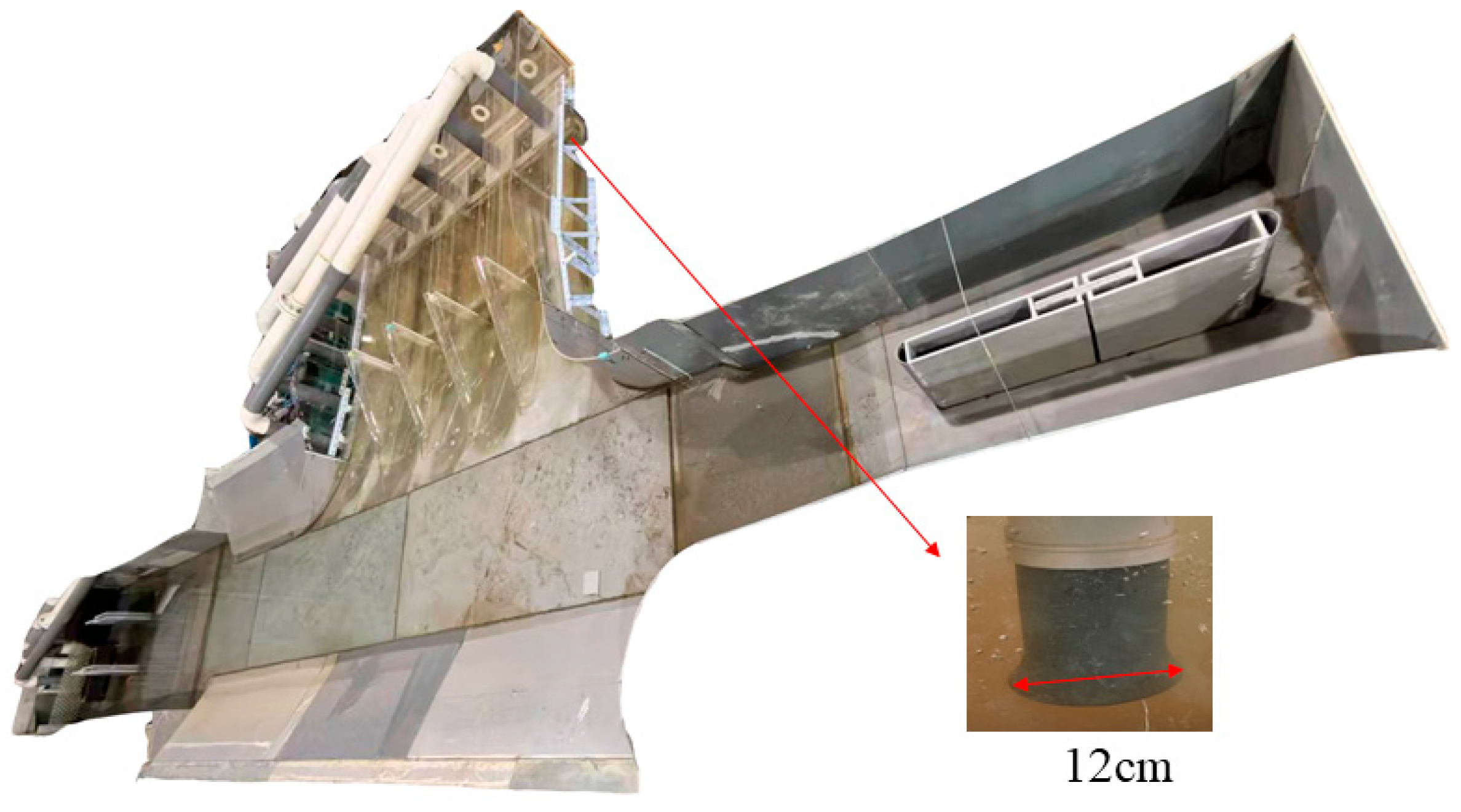
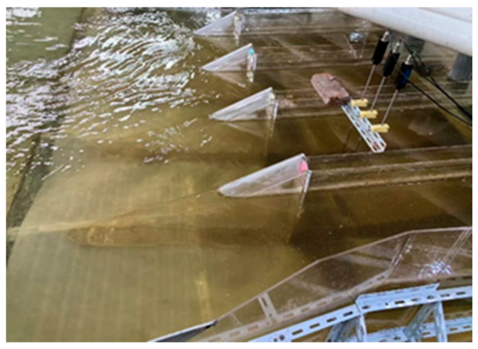
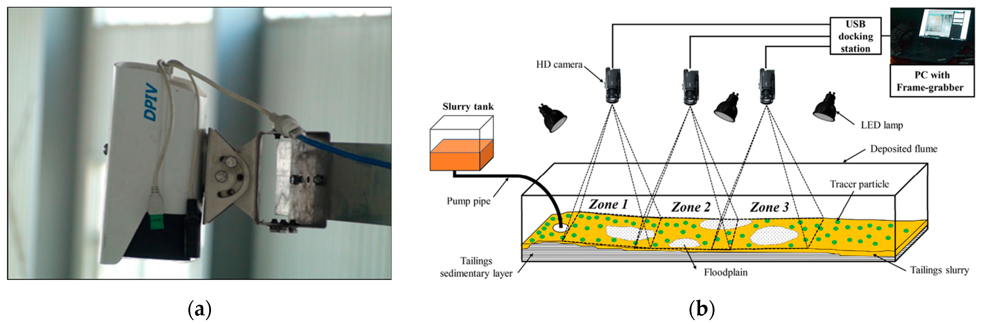
2.2. Physical Model
2.2.1. Similarity Criterion
2.2.2. Model Layout
2.3. Numerical Simulation
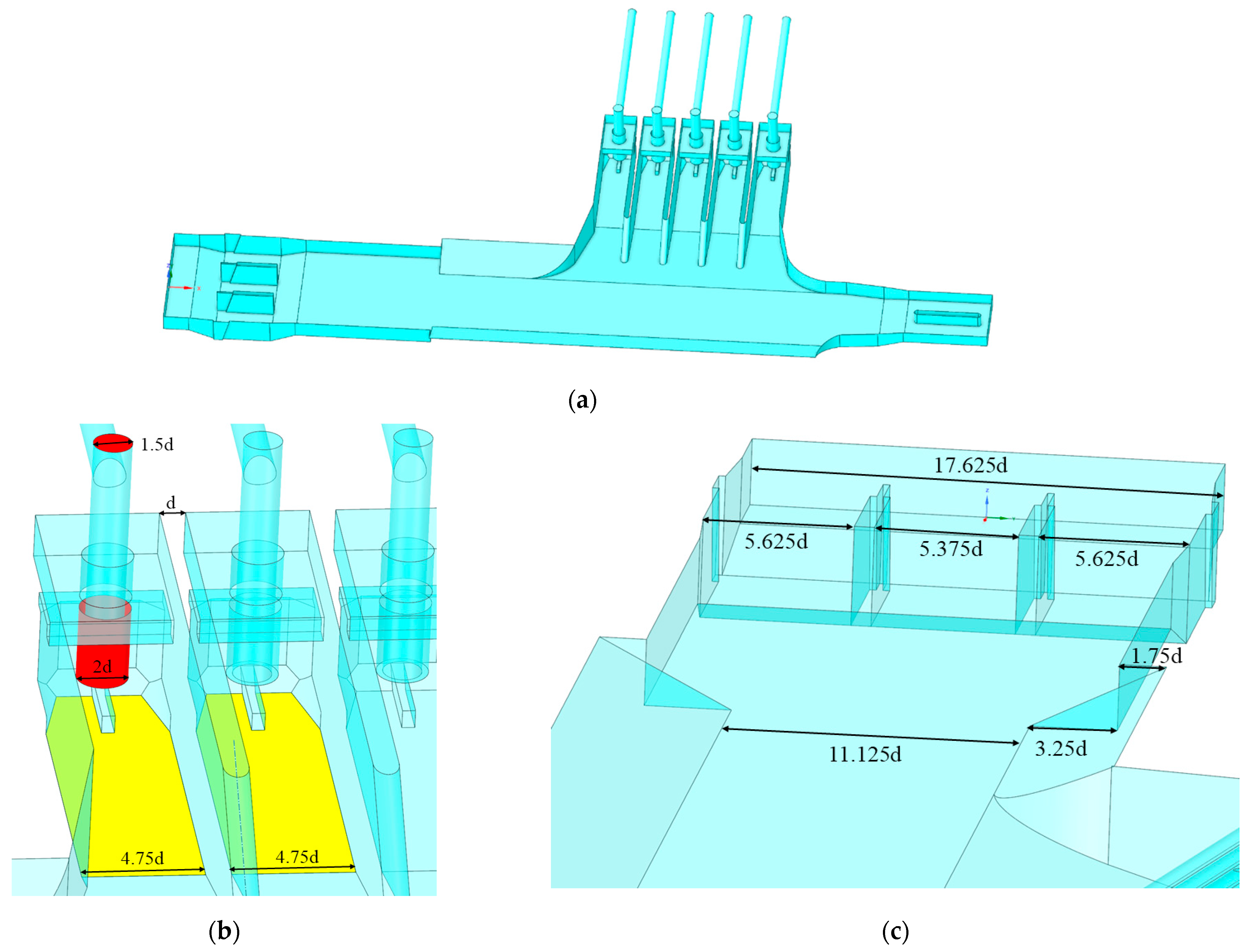
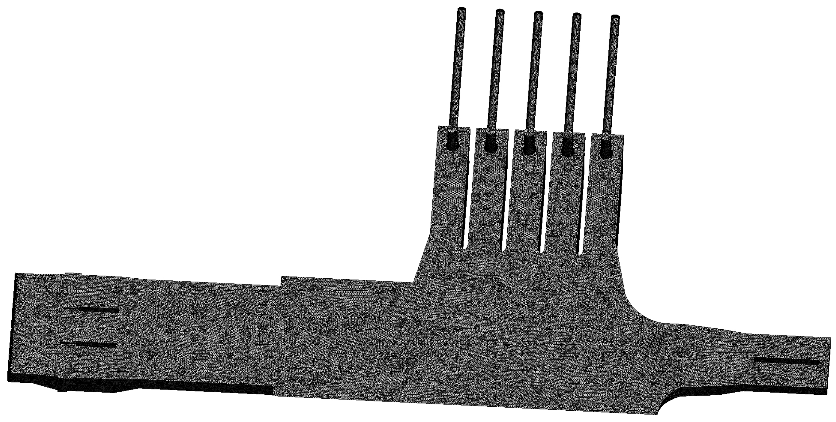
2.3.1. Geometric Model
2.3.2. Governing Equations and Turbulent Flow Models
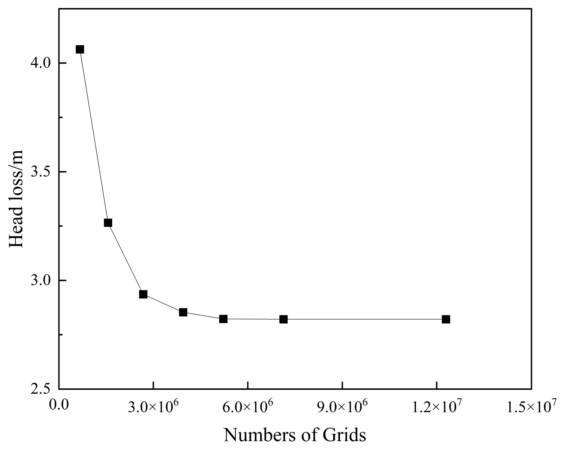
2.3.3. Grid Independence Analysis
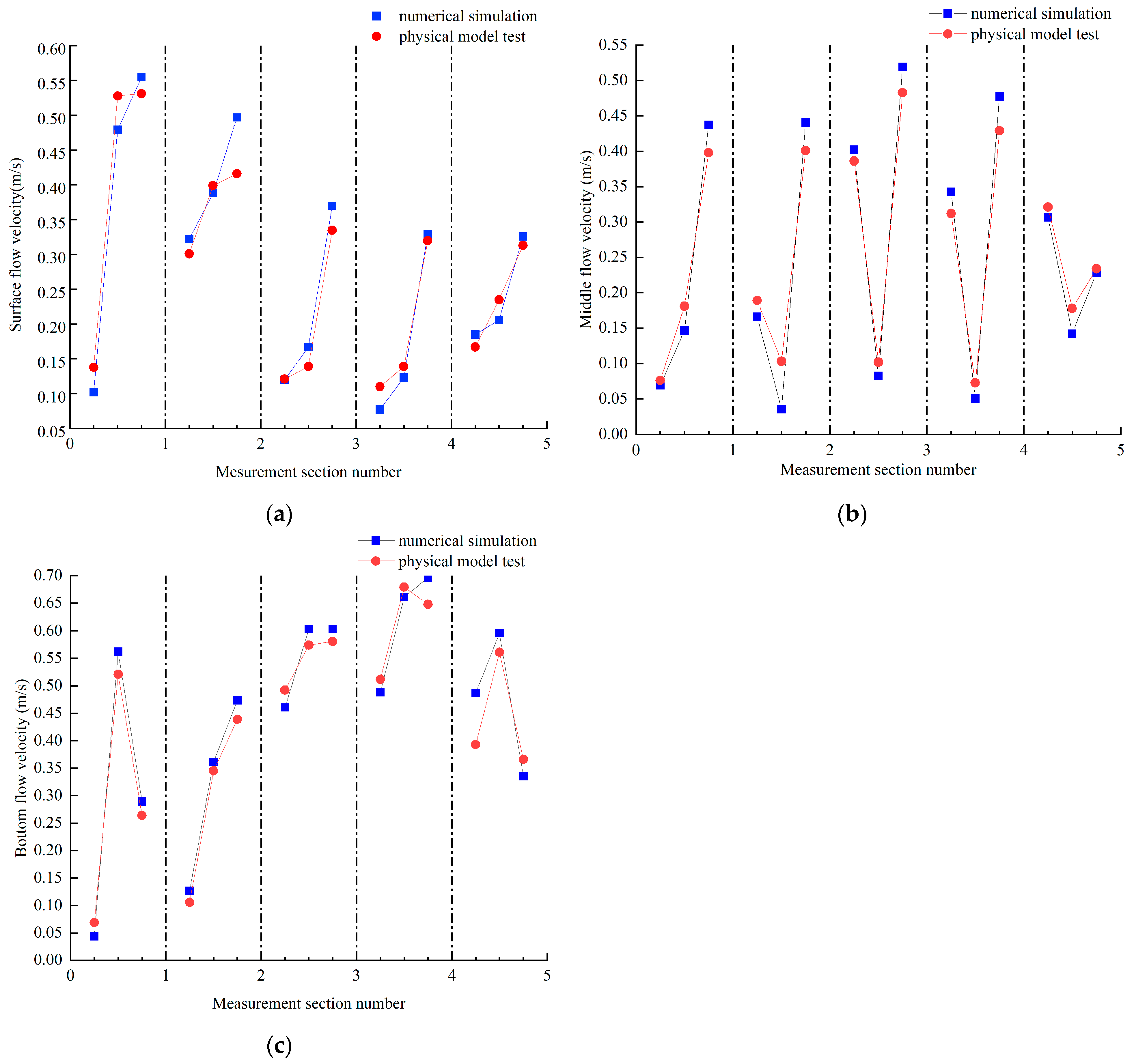
2.3.4. Verification of the Numerical Simulation’s Reliability
3. Analysis and Discussion
3.1. Optimizing Program Design
3.2. Hydraulic Characteristic Analysis
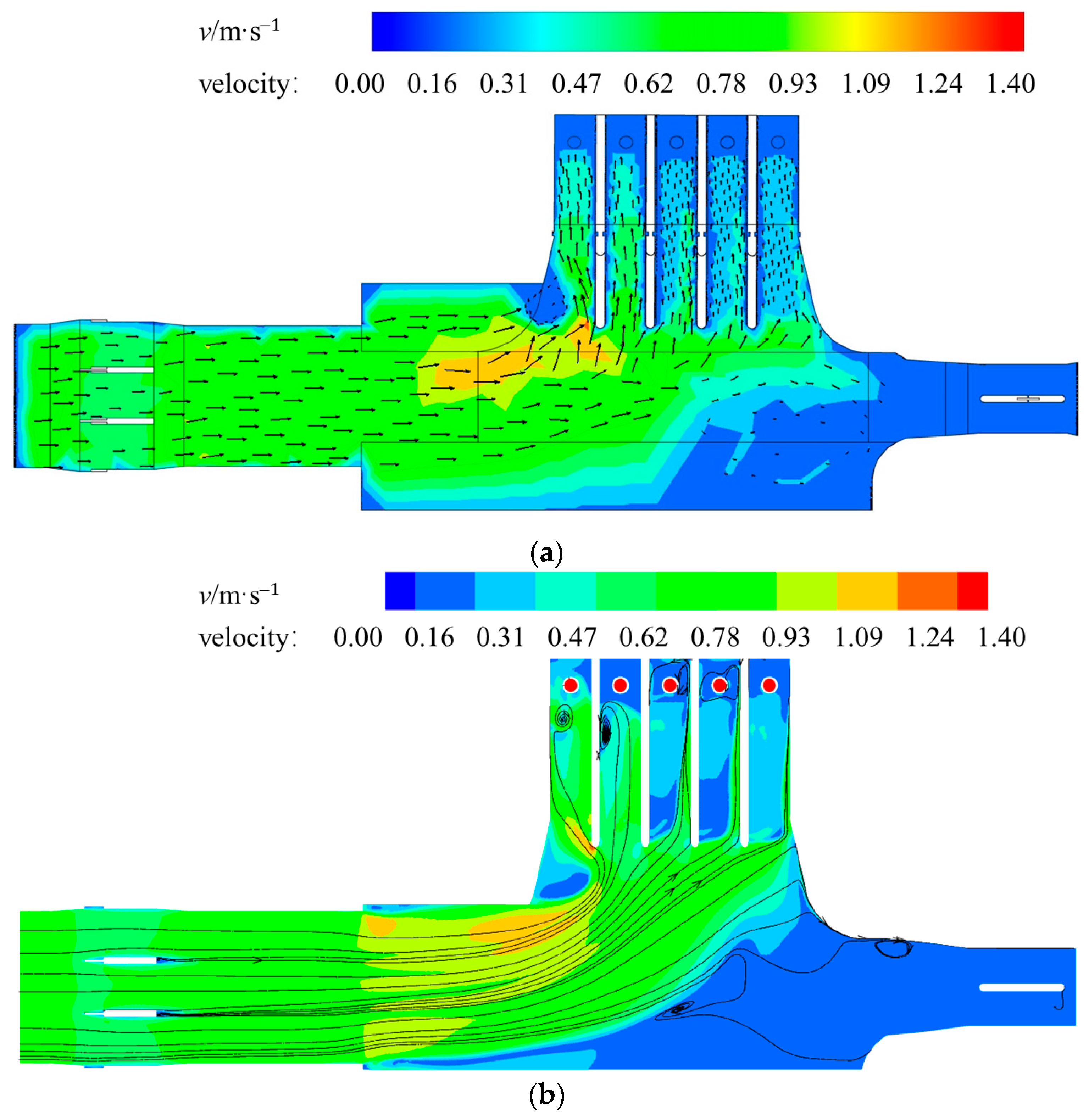
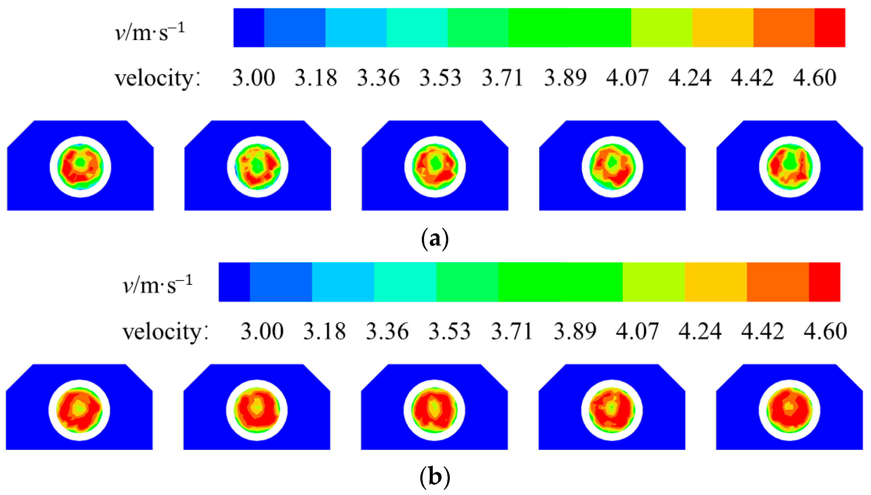
3.2.1. Original Scheme
3.2.2. Optimization Scheme 1
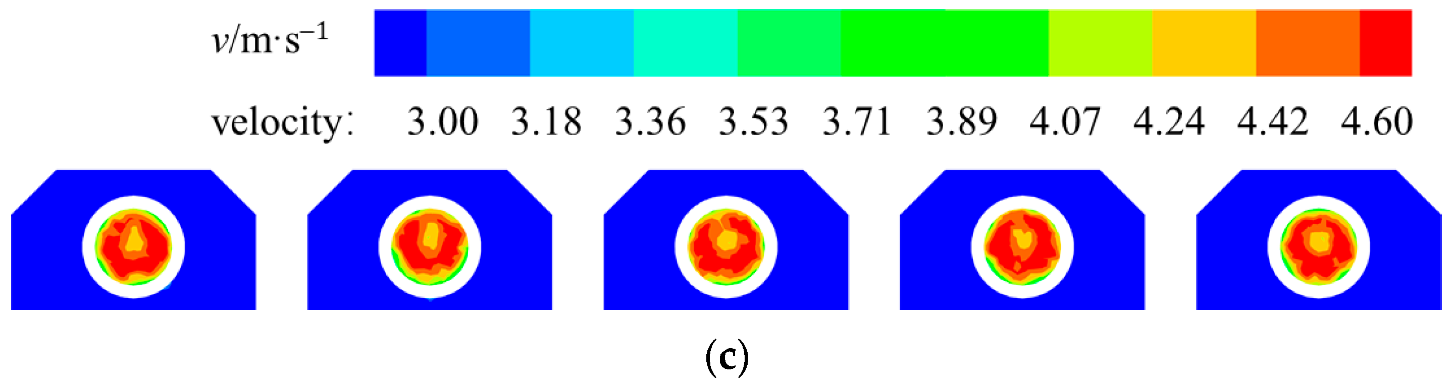
3.2.3. Optimization Scheme 2
3.3. Quantitative Evaluation of the Optimization Effect
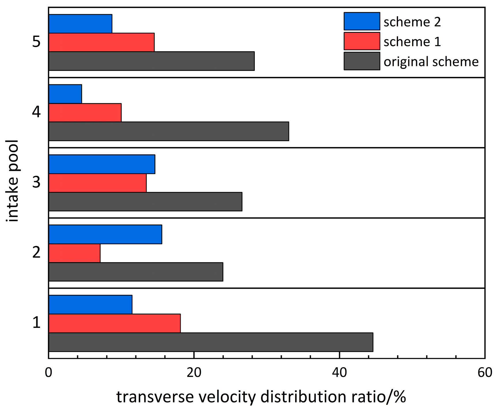
3.3.1. Transverse Velocity Distribution Ratio
3.3.2. Axial Velocity Weighted Average Angle and Axial Velocity Uniformity
3.4. Optimal Scheme Determination
3.5. Response Surface Methodology to Optimize Parameter Design
4. Conclusions
- In the absence of optimization measures for the original conditions, the pumping station inlet pool is subject to undesirable flow conditions, including bias flow and return flow. Furthermore, the flow velocity distribution is characterized by significant unevenness. This will increase the head loss, affect the pumping unit’s intake efficiency, reduce the efficiency of the pumping station, and shorten the working life of the pumping unit.
- Scheme 1 and scheme 2 have been shown to be effective in improving the flow pattern in the inlet pool of the pumping station. However, it is optimized scheme 2 that has been demonstrated to have a superior rectification effect. The lateral flow velocity distribution ratio of the pumping station under scheme 2 is reduced by 20.305%, the axial flow uniformity is improved by 52.24%, the weighted mean axial flow angle is improved by 5.92°, and the mean square error MSE is reduced by 0.621. This indicates that the rectification effect of scheme 2 is superior to that of scheme 1. In this study, the response surface method is employed to ascertain the optimal distribution of the separation distance of the separation pier under the optimized scheme 2. The flow uniformity is enhanced by 2.23% in comparison with scheme 2, and the inlet pool exhibits a superior rectification effect. The flow uniformity is enhanced by 2.23% in comparison with scheme 2, and the flow pattern in the inlet pool is further optimized.
- This study puts forward a series of evaluation indices that are of great significance for the qualitative and quantitative analysis of flow patterns in hydraulic tests. It is evident that, in flow analysis, the pumping station inlet pool and the front pool play a significant role in guiding the selection of different optimization schemes. A comparison between these selection schemes provides a substantial amount of powerful data support. The design stage of pumping stations is often constrained by limitations relating to the available urban land, as well as numerous environmental factors. This study proposes a novel guide wall and guide pier amalgamation rectification strategy. In a lateral-intake pumping station inlet pool in a truncated-type river, the rectification effect is enhanced by poor flow patterns. The rectification of similar pumping stations with a small forebay or no forebay provides a certain degree of guidance.
- This study is founded upon a project simulation. The rectification scheme that has been proposed has geometric parameters designed for special characteristics, and it is necessary for these to be combined with the geometric parameters of a pumping station in similar cases. The same is true for the flow rate or flow direction in the corresponding empirical formulas. Subsequent studies could examine the interactions between various optimization features, such as the angle between the deflector wall and the main flow line, the curvature of the fan-shaped deflector piers, and the direction of the interval segments of the separating deflector wall.
Author Contributions
Funding
Data Availability Statement
Conflicts of Interest
Appendix A

| Symbol | Physical Meaning | Unit |
|---|---|---|
| length | m | |
| area | m2 | |
| volume | m3 | |
| scale | / | |
| prototype | / | |
| model | / | |
| time | s | |
| flow rate | m3/s | |
| gravity | N | |
| water density | Kg/m3 | |
| mass | Kg | |
| similarity scale | / | |
| roughness | / | |
| flow rate | cm/s | |
| flow rate signal frequency | r/s | |
| curve slope | / | |
| coefficient | cm/s | |
| velocity vector | / | |
| coordinate axis | / | |
| static pressure | pa | |
| effective viscosity coefficient | / | |
| gravity component | / | |
| , | turbulent kinetic energy | / |
| dissipation | / | |
| turbulence Prandtl number | / | |
| gravity | N/Kg | |
| hydraulic loss | m | |
| mean square error | / | |
| velocity | m/s | |
| uniformity | / | |
| axial velocity | m/s | |
| angle of axial flow | ° | |
| root mean square error | / |
References
- Nasr, A.; Yang, F.; Zhang, Y.Q.; Wang, T.L.; Hassan, M. Analysis of the Flow Pattern and Flow Rectification Measures of the Side-Intake Forebay in a Multi-Unit Pumping Station. Water 2021, 13, 2025. [Google Scholar] [CrossRef]
- Xi, W.; Lu, W.G.; Wang, C.; Liu, J.F. Analysis of Pumping Station Inlet Characteristics Based on Vorticity. Int. J. Simul. Model. 2022, 21, 453–464. [Google Scholar] [CrossRef]
- Alvez, A.; Espinosa, P.; Castillo, R.; Iglesias, K.; Bañales-Seguel, C. An Urgent Dialogue between Urban Design and Regulatory Framework for Urban Rivers: The Case of the Andalien River in Chile. Water 2022, 14, 3444. [Google Scholar] [CrossRef]
- Xu, C.; Zhang, H.; Zhang, X.; Han, L.; Wang, R.; Wen, Q.; Ding, L. Numerical Simulation of the Impact of Unit Commitment Optimization and Divergence Angle on the Flow Pattern of Forebay. Int. J. Heat Technol. 2015, 33, 91–96. [Google Scholar] [CrossRef]
- Song, W.; Pang, Y.; Shi, X.; Xu, Q. Study on the Rectification of Forebay in Pumping Station. Math. Probl. Eng. 2018, 2018, 1–16. [Google Scholar] [CrossRef]
- Tsai, Y.S.; Chang, Y.M.; Chang, Y.J.; Chen, Y.M. Phase-Resolved Piv Measurements of the Flow between a Pair of Corotating Disks in a Cylindrical Enclosure. J. Fluids Struct. 2007, 23, 191–206. [Google Scholar] [CrossRef]
- Chen, T.D. An Affine-Model-Based Technique for Fast Dpiv Computation. Image Vis. Comput. 2006, 24, 407–410. [Google Scholar]
- Wijesooriya, K.; Mohotti, D.; Lee, C.K.; Mendis, P. A Technical Review of Computational Fluid Dynamics (Cfd) Applications on Wind Design of Tall Buildings and Structures: Past, Present and Future. J. Build. Eng. 2023, 74, 106828. [Google Scholar] [CrossRef]
- Blocken, B. Computational Fluid Dynamics for Urban Physics: Importance, Scales, Possibilities, Limitations and Ten Tips and Tricks Towards Accurate and Reliable Simulations. Build. Environ. 2015, 91, 219–245. [Google Scholar] [CrossRef]
- Al-Obaidi, A.R. Evaluation and Investigation of Hydraulic Performance Characteristics in an Axial Pump Based on Cfd and Acoustic Analysis. Processes 2024, 12, 129. [Google Scholar] [CrossRef]
- Choi, J.-W.; Choi, Y.-D.; Kim, C.-G.; Lee, Y.-H. Flow Uniformity in a Multi-Intake Pump Sump Model. J. Mech. Sci. Technol. 2010, 24, 1389–1400. [Google Scholar] [CrossRef]
- Dimas Athanassios, A.; Andreas, P.V. Effect of Cross-Flow Velocity at Forebay on Swirl in Pump Suction Pipe: Hydraulic Model of Seawater Intake at Aliveri Power Plant in Greece. J. Hydraul. Eng. 2012, 138, 812–816. [Google Scholar] [CrossRef]
- Rajendran, V.P.; Constantinescu, S.G.; Patel, V.C. Experimental Validation of Numerical Model of Flow in Pump-Intake Bays. J. Hydraul. Eng.-ASCE 1999, 125, 1119–1125. [Google Scholar] [CrossRef]
- Zhang, C.; Yan, H.; Jamil, M.T.; Yu, Y. Improvement of the Flow Pattern of a Forebay with a Side-Intake Pumping Station by Diversion Piers Based on Orthogonal Test Method. Water 2022, 14, 2663. [Google Scholar] [CrossRef]
- Yang, F.; Zhang, Y.; Liu, C.; Wang, T.; Jiang, D.; Jin, Y. Numerical and Experimental Investigations of Flow Pattern and Anti-Vortex Measures of Forebay in a Multi-Unit Pumping Station. Water 2021, 13, 935. [Google Scholar] [CrossRef]
- Li, J.; Zhou, J.; Xu, H.; Feng, J.; Tong, H.; Chen, Y.; Qian, S. Undesired Flows in Lateral-Intake Multiple Forebays and Their Hydraulic Implications: Case Study for Asia’s Largest Urban Water Supply Pumping Station. Eng. Appl. Comput. Fluid Mech. 2024, 18, 2380304. [Google Scholar] [CrossRef]
- Wang, H.D.; Xu, D.; Ding, C.F.; Ran, Q.H.; Yuan, S.Y.; Tang, H.W. Numerical and Experimental Study on Water-Sediment Flow in a Lateral Pumping Station Forebay. Phys. Fluids 2024, 36, 095162. [Google Scholar] [CrossRef]
- Qiao, Q.; Wang, H.D.; Huang, L.X.; Jing, H.F.; Wang, B.Y. Impact of Inlet Flow Velocity on Sediment Reduction in Pump Station Forebays. Phys. Fluids 2024, 36, 115183. [Google Scholar] [CrossRef]
- Luo, C.; Zhang, L.; Wang, T.L.; Liu, H.; Cheng, L.; Lu, M.Z.; Jiao, W.X. Vortex Energy Behaviors in the Forebay of Lateral Pumping Station for Y-Type Channel. Phys. Fluids 2024, 36, 075162. [Google Scholar] [CrossRef]
- Olszewski, P. Genetic Optimization and Experimental Verification of Complex Parallel Pumping Station with Centrifugal Pumps. Appl. Energy 2016, 178, 527–539. [Google Scholar] [CrossRef]
- Banaszek, A.; Losiewicz, Z.; Jurczak, W. Corrosion Influence on Safety of Hydraulic Pipelines Installed on Decks of Contemporary Product and Chemical Tankers. Pol. Marit. Res. 2018, 25, 71–77. [Google Scholar] [CrossRef]
- Caishui, H.O.U. Three-Dimensional Numerical Analysis of Flow Pattern in Pressure Forebay of Hydropower Station. Procedia Eng. 2012, 28, 128–135. [Google Scholar] [CrossRef]
- Shaheed, R.; Mohammadian, A.; Gildeh, H.K. A Comparison of Standard K–Ε and Realizable K–Ε Turbulence Models in Curved and Confluent Channels. Environ. Fluid Mech. 2019, 19, 543–568. [Google Scholar] [CrossRef]
- Wang, H.D.; Li, C.G.; Lu, S.J.; Yang, C.; Huang, L.X. Numerical and Experimental Study on Vortex Optimization in the Forebay of a Sandy River. Phys. Fluids 2023, 35, 085128. [Google Scholar] [CrossRef]
- Liu, J.Y.; Heidarinejad, M.; Pitchurov, G.; Zhang, L.H.; Srebric, J. An Extensive Comparison of Modified Zero-Equation, Standard K-Ε, and Les Models in Predicting Urban Airflow. Sustain. Cities Soc. 2018, 40, 28–43. [Google Scholar] [CrossRef]
- Lateb, M.; Masson, C.; Stathopoulos, T.; Bédard, C. Comparison of Various Types of K-Ε Models for Pollutant Emissions around a Two-Building Configuration. J. Wind Eng. Ind. Aerodyn. 2013, 115, 9–21. [Google Scholar] [CrossRef]
- Zhan, J.-M.; Wang, B.-C.; Yu, L.-H.; Li, Y.-S.; Tang, L. Numerical Investigation of Flow Patterns in Different Pump Intake Systems. J. Hydrodyn. 2012, 24, 873–882. [Google Scholar] [CrossRef]
- Xu, B.; Liu, J.F.; Lu, W.G. Optimization Design of Y-Shaped Settling Diversion Wall Based on Orthogonal Test. Machines 2022, 10, 91. [Google Scholar] [CrossRef]
- Zhou, J.R.; Zhao, M.M.; Wang, C.; Gao, Z.J. Optimal Design of Diversion Piers of Lateral Intake Pumping Station Based on Orthogonal Test. Shock Vib. 2021, 2021, 6616456. [Google Scholar] [CrossRef]
- Chen, Y.-X.; Xi, B.; Chen, Z.; Shen, S. Study on the Hydraulic Characteristics of an Eccentric Tapering Outlet Pressure Box Culvert in a Pumping Station. Processes 2023, 11, 1598. [Google Scholar] [CrossRef]


| Scheme | Plan View of the Optimization Measure of the Deflector Piers (Unit: cm) | Dimension | |
|---|---|---|---|
| Original |  | ||
| 1 | 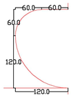 |  | |
| 2 |  | 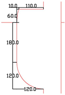 |  |
| Scheme | Section | |
|---|---|---|
| /% | θa/° | |
| Original scheme | 17.50 | 77.17 |
| Scheme1 | 62.53 | 82.69 |
| Scheme2 | 69.74 | 83.09 |
| Run | Factor 1 (L1/cm) | Factor 2 (L2/cm) | Factor 3 (L3/cm) | Response (Axial Velocity Uniformity) |
|---|---|---|---|---|
| 1 | 160 | 160 | 190 | 64.49 |
| 2 | 180 | 160 | 190 | 65.93 |
| 3 | 160 | 180 | 190 | 68.3 |
| 4 | 180 | 180 | 190 | 66.55 |
| 5 | 160 | 170 | 180 | 69.94 |
| 6 | 180 | 170 | 180 | 69.56 |
| 7 | 160 | 170 | 200 | 65.6 |
| 8 | 180 | 170 | 200 | 64.69 |
| 9 | 170 | 160 | 180 | 69.32 |
| 10 | 170 | 180 | 180 | 69.74 |
| 11 | 170 | 160 | 200 | 64.03 |
| 12 | 170 | 180 | 200 | 68.66 |
| 13 | 170 | 170 | 190 | 71.39 |
| 14 | 170 | 170 | 190 | 71.04 |
| 15 | 170 | 170 | 190 | 71.68 |
| Source | Sum of Squares | df | Mean Square | F-Value | p-Value |
|---|---|---|---|---|---|
| Model | 95.52 | 9 | 10.61 | 38.40 | 0.0004 |
| A-L1 | 0.3200 | 1 | 0.3200 | 1.16 | 0.3310 |
| B-L2 | 11.23 | 1 | 11.23 | 40.65 | 0.0014 |
| C-L3 | 30.34 | 1 | 30.34 | 109.80 | 0.0001 |
| AB | 2.54 | 1 | 2.54 | 9.21 | 0.0289 |
| AC | 0.0702 | 1 | 0.0702 | 0.2541 | 0.6356 |
| BC | 4.43 | 1 | 4.43 | 16.03 | 0.0103 |
| A2 | 28.36 | 1 | 28.36 | 102.61 | 0.0002 |
| B2 | 19.22 | 1 | 19.22 | 69.53 | 0.0004 |
| C2 | 4.89 | 1 | 4.89 | 17.71 | 0.0084 |
| Residual | 1.38 | 5 | 0.2763 | ||
| Lack of Fit | 1.18 | 3 | 0.3921 | 3.82 | 0.2145 |
| Pure Error | 0.2054 | 2 | 0.1027 | ||
| Cor Total | 96.90 | 14 |
Disclaimer/Publisher’s Note: The statements, opinions and data contained in all publications are solely those of the individual author(s) and contributor(s) and not of MDPI and/or the editor(s). MDPI and/or the editor(s) disclaim responsibility for any injury to people or property resulting from any ideas, methods, instructions or products referred to in the content. |
© 2025 by the authors. Licensee MDPI, Basel, Switzerland. This article is an open access article distributed under the terms and conditions of the Creative Commons Attribution (CC BY) license (https://creativecommons.org/licenses/by/4.0/).
Share and Cite
Ji, R.; Xi, B.; Lian, Y.; Song, Z. A Study on the Inlet Characteristics of a 90° Lateral-Inlet Pumping Station with a Truncated River. Water 2025, 17, 1806. https://doi.org/10.3390/w17121806
Ji R, Xi B, Lian Y, Song Z. A Study on the Inlet Characteristics of a 90° Lateral-Inlet Pumping Station with a Truncated River. Water. 2025; 17(12):1806. https://doi.org/10.3390/w17121806
Chicago/Turabian StyleJi, Rui, Bin Xi, Yanxu Lian, and Zihao Song. 2025. "A Study on the Inlet Characteristics of a 90° Lateral-Inlet Pumping Station with a Truncated River" Water 17, no. 12: 1806. https://doi.org/10.3390/w17121806
APA StyleJi, R., Xi, B., Lian, Y., & Song, Z. (2025). A Study on the Inlet Characteristics of a 90° Lateral-Inlet Pumping Station with a Truncated River. Water, 17(12), 1806. https://doi.org/10.3390/w17121806