Article

Application of LSTM and Climate Index for Prediction of Meteorological Drought in South Korea

Department of Civil Engineering, Chosun University, Gwangju 61452, Republic of Korea
*
Author to whom correspondence should be addressed.
Water 2025, 17(12), 1801; https://doi.org/10.3390/w17121801
Submission received: 30 April 2025 / Revised: 29 May 2025 / Accepted: 13 June 2025 / Published: 16 June 2025

Abstract

:
Climate change has intensified natural hazards, including droughts, which have caused substantial damage in South Korea. Drought, characterized by prolonged moisture deficiency, is typically assessed using drought indices that reflect meteorological conditions. This study examined the influence of various meteorological and climate indices on drought variability in the Yeongsan and Seomjin River basins. The Standardized Precipitation Index (SPI) was used to represent drought conditions, and its monthly variations were predicted using the Long Short-Term Memory (LSTM) algorithm. To assess model performance, four statistical indicators—Mean Squared Error (MSE), Root Mean Squared Error (RMSE), Nash–Sutcliffe Efficiency (NSE), and the Coefficient of Determination (R2)—were employed. The LSTM model that utilized both precipitation and drought indices as input data showed the best performance, achieving an MSE of 0.2, RMSE of 0.477, NSE of 0.77, and R2 of 0.78. Overall predictive performance ranged from 0.298 to 0.347 (MSE), 0.546 to 0.589 (RMSE), 0.578 to 0.628 (NSE), and 0.580 to 0.675 (R2). This study highlights the effectiveness of LSTM in predicting drought conditions and the value of incorporating meteorological and climatic indices. The results can support improved drought hazard assessment and management strategies in South Korea.

1. Introduction

Recently, owing to climate change, the importance of research on natural hazards has been highlighted. According to Zittis et al. (2014) [1], various natural hazards caused by climate change have significant impacts on society, the environment, water resources, and ecosystems, making it crucial to predict and manage these events.
With the advancement of computer technology, Samuel (1959) [2] proposed machine learning techniques, which are defined as a field of study that gives computers the ability to learn without being explicitly programmed. In other words, it is the process of achieving a task through experiences obtained in the form of data.
Machine learning can be broadly divided into two categories based on the learning methods: supervised and unsupervised learning. Representative algorithms for supervised learning include Artificial Neural Networks (ANNs) [3], naïve Bayes [4], Random Forest [5], and Support Vector Machines [6]. For unsupervised learning, notable algorithms include nonnegative matrices [7], Hierarchical Clustering Schemes [8], Uniform Manifold Approximation and Projection [9], and K-Means Clustering [10]. In this study, the Long Short-Term Memory (LSTM) algorithm [11] was used in supervised learning to predict data.
Owing to the rapidly changing meteorological conditions, studies on drought prediction using machine learning, which utilizes meteorological indices as input values, have been performed. For instance, Feng et al. (2019) [12] used 30 remote sensing-based environmental factors from 2001 to 2017 in southeastern New South Wales to predict the ground-based climate indices and Standardized Precipitation Evapotranspiration Index (SPEI) using Random Forest, Support Vector Machine, and Multilayer Perceptron. They concluded that the Random Forest algorithm demonstrated the highest performance with Root Mean Squared Error (RMSE) = 0.28 and R-squared (R2) = 0.9. Rahmati et al. (2020) [13] evaluated the importance of hydrological environmental factors in predicting the agricultural drought risk in southeastern Queensland, Australia, from 1994 to 2013, using machine learning algorithms. They showed that the Random Forest algorithm achieved the highest accuracy, with an area under the receiver operating characteristic curve of 97.7%, a True Skill Statistic of 0.873, an efficiency of 0.929, and an F-score of 0.898.
Tyagi et al. (2022) [14] analyzed the impact of drought on agricultural systems and investigated the performance of machines and deep learning in predicting drought events. Mokhtar et al. (2021) [15] proposed a method for analyzing drought in the Tibetan Plateau, China, from 1980 to 2019 by combining SPEI with four machine learning algorithms: Random Forest, Extreme Gradient Boost, Convolutional Neural Network, and LSTM. They utilized SPI3 and SPI6 as input data for machine learning algorithms to predict SPEI variability. Zhang et al. (2019) [16] developed a model to predict the SPEI using meteorological factors and climate indices observed from 1961 to 2016 and employed a distributed lag nonlinear model, ANN, and Extreme Gradient Boosting. The Extreme Gradient Boosting model showed the predictive performance with R2 values ranged 0.68–0.82, 0.72–0.89, 0.81–0.92, and 0.84–0.95 for 3-, 6-, 9-, and 12-month scales, respectively. In addition, Karbasi et al. (2023) [17] predicted the SPEI using data from two synoptic weather stations, Tabriz and Rasht, between 1987 and 2019, combining the empirical wavelet transform, discrete wavelet transforms, and Multilayer Perceptron with an extended Kalman filter. This combination showed superior predictive performance at both stations.
Climate change is defined as long-term variations in various climate characteristics, such as solar activity cycles, atmospheric composition changes, and land-use changes. These changes have led to meteorological anomalies observed since the 1950s, resulting in numerous natural hazards that significantly affect ecosystems. Global warming has altered the hydrological cycle, causing shifts in precipitation patterns around the world [18]. Consequently, flood frequency has increased in high-latitude and equatorial regions, while the occurrence of droughts is projected to rise in mid-latitude and subtropical areas. As the frequency of droughts increases due to changing climate patterns, research utilizing climate indices has become a critical task.
Shamshirband et al. (2020) [19] conducted drought index modeling using the SPI, Standardized Streamflow Index (SSI), and SPEI for hydrological drought modeling with Support Vector Regression, Gene Expression Programming, and M5 Model Tree. The study found that the SPI provided the highest accuracy for hydrological drought modeling, with the MT model showing high performance in SSI prediction correlation coefficient = 0.8175 and RMSE = 0.8186. Belayneh and Adamowski (2013) [20] used SPI as input data to predict short-term droughts in the Awash River Basin in Ethiopia. They employed ANN, Support Vector Regression, and Wavelet Analysis to preprocess input data using a combined wavelet ANN approach to predict future droughts. However, existing studies have used meteorological indices within the study area as input data, which presents challenges in explaining the impacts of climate change. Kim and Kim (2021) [21] conducted a rainfall-runoff analysis by applying the Soil and Water Assessment Tool (SWAT) and LSTM using meteorological and topographical indices in the Yeongsan River Basin, which forms a large-scale agricultural area. The results indicated that LSTM demonstrated a higher performance than the SWAT model in rainfall-runoff analysis, as evaluated by the Nash–Sutcliffe Efficiency (NSE) index.
This study focuses on the Yeongsan and Seomjin River Basins in South Korea and aims to predict the meteorological drought index SPI using both climate and meteorological indices through the LSTM algorithm. While previous research in these regions has primarily focused on agricultural water management, disaster-related studies such as drought prediction have largely relied on topographical and meteorological indices. In this study, climate indices were additionally incorporated to evaluate their impact on drought disaster prediction. Early prediction of drought is crucial for minimizing damage, and the findings of this study provide fundamental data for responding to drought disasters while also highlighting the applicability of machine learning-based drought prediction models.

2. Materials and Methods

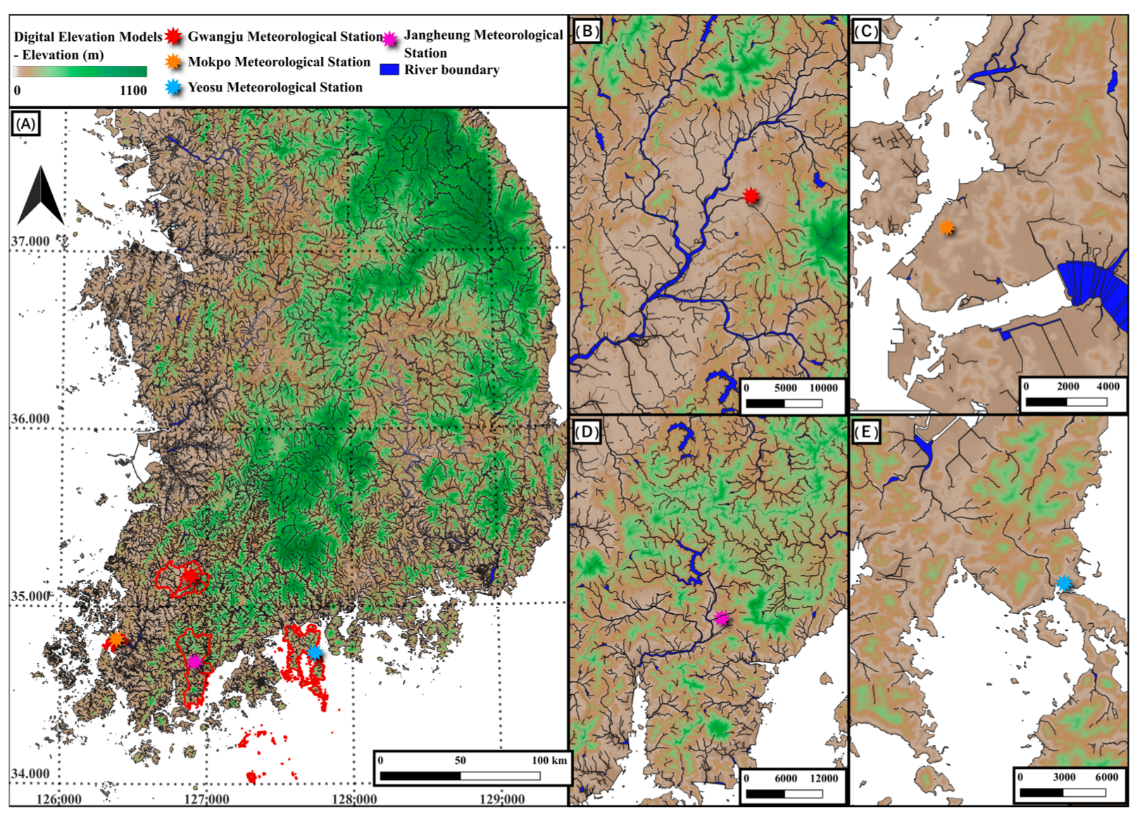
2.1. Study Area Information

The Yeongsan River Basin is one of the four major river basins in South Korea, with a main river length of approximately 150 km and a basin area of 3551 km. Owing to its predominantly plain topography, water resources in the basin are primarily utilized for agricultural purposes. The Seomjin River Basin has a main river length of 212.3 km and a basin area of 4896.5 km2 and is located to the east of the Yeongsan River Basin. Both the Yeongsan and Seomjin River Basins cover most of Jeollanam-do Province, South Korea. A recent drought event that affected multiple major cities in this region was reported in March 2022 [22].
This study selected the Yeongsan and Seomjin River basins in Jeollanam-do, South Korea, as the target regions. Specifically, the analysis focused on sub-basins that had previously experienced drought conditions, including Gwangju, Mokpo, and Jangheung in the Yeongsan River Basin, and Yeosu in the Seomjin River Basin (Figure 1). These sub-basins were selected based on the availability of meteorological stations that provide the SPI, as well as the continuity and completeness of long-term climate records. Although these stations are not streamflow (hydrological) observation points, their data are suitable for SPI-based analysis and, thus, align with the aims of this study. However, there may be some limitations in spatial representativeness that can be addressed through additional data and future improvements.
The selection of these sub-basins is also supported by their relevance to regional drought management. While broader basins are of strategic agricultural importance, these specific sub-basins have been notably impacted by recent droughts and are representative of varying hydrometeorological conditions within larger watersheds. This provides a focused and meaningful scope for evaluating drought characteristics. Moreover, although previous studies have addressed SPI prediction using climatic variables, this study distinguishes itself by applying this methodology to historically drought-affected regions with specific geographical and data constraints to assess the applicability of such models under real-world limitations, contributing to more localized drought risk management strategies.

2.2. Datasets

2.2.1. Data Information

In this study, the SPI data calculated using precipitation data provided by the Korea Meteorological Administration: https://data.kma.go.kr (accessed on 23 January 2024) was used [23]. A drought index based solely on precipitation was developed to assess drought severity, offering the advantage of flexibly representing both short- and long-term droughts by indicating precipitation surplus or deficit over time [24]. Kim and Lee (2011) [25] selected SPI3 as the most effective index for drought analysis in Korea through correlation analysis. For this study, SPI3, which represents the cumulative precipitation over a 3-month period, was used. SPI3 values, calculated from meteorological observations at stations in Gwangju City, Mokpo City, Yeosu City, and Jangheung County, were collected and applied for the period of 1991–2022.
Meteorological data provided by the Automated Synoptic Observing System (ASOS) of the Korea Meteorological Administration were used (Table 1). Surface meteorological observations refer to ground-based observational data collected simultaneously at 105 meteorological stations across the country at specific times to understand the regional weather conditions. For this study, ASOS data (including 12 variables, such as average temperature and local pressure) were collected from four meteorological stations in the research area and applied to the LSTM model after preprocessing. To ensure data reliability, only data with <10% missing values were used. If missing values were present in the SPI3 or meteorological indices, they were handled using the monthly mean imputation method. Missing values were replaced with the monthly average of the corresponding variables at each station to ensure data continuity and reduce potential bias in the analysis.

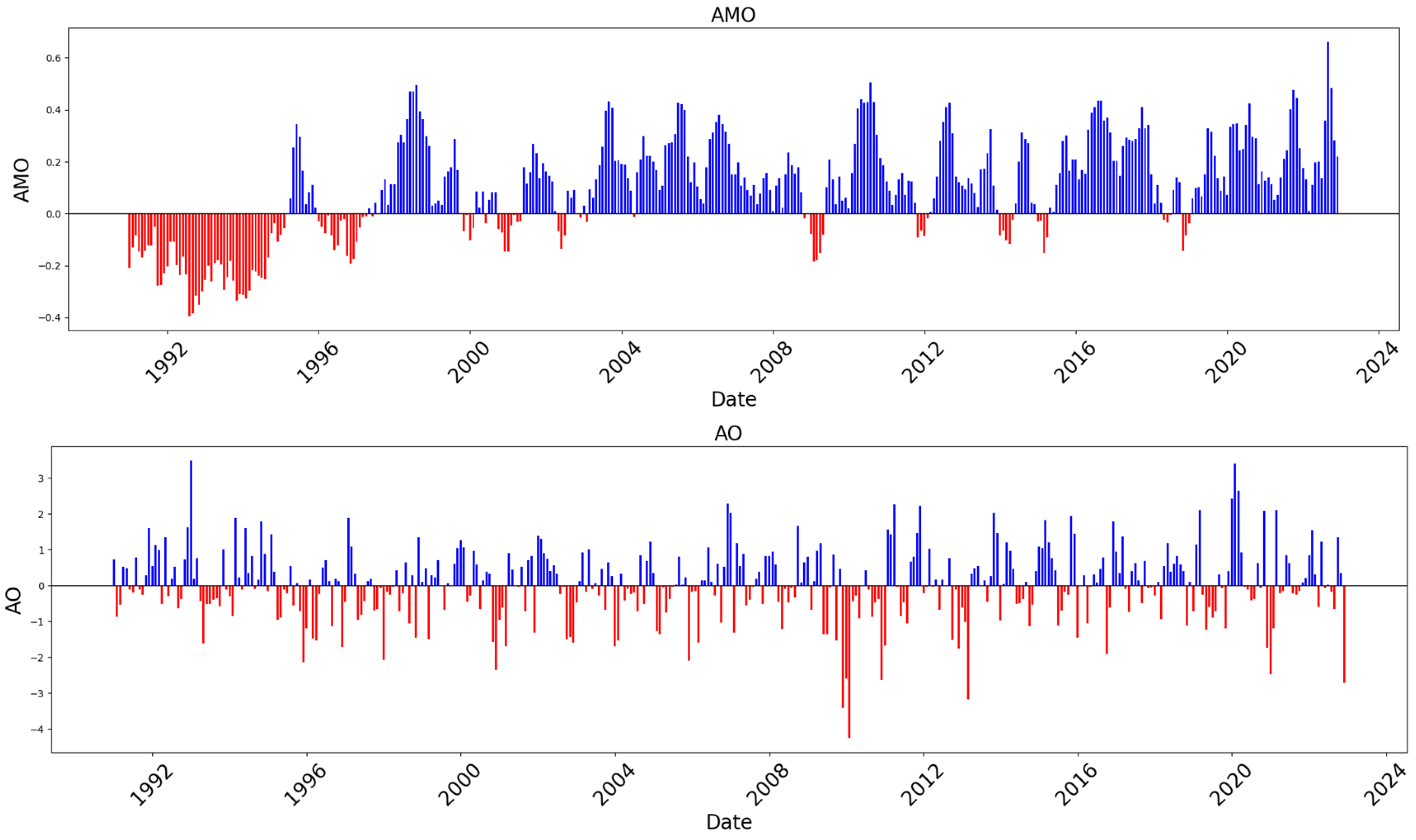
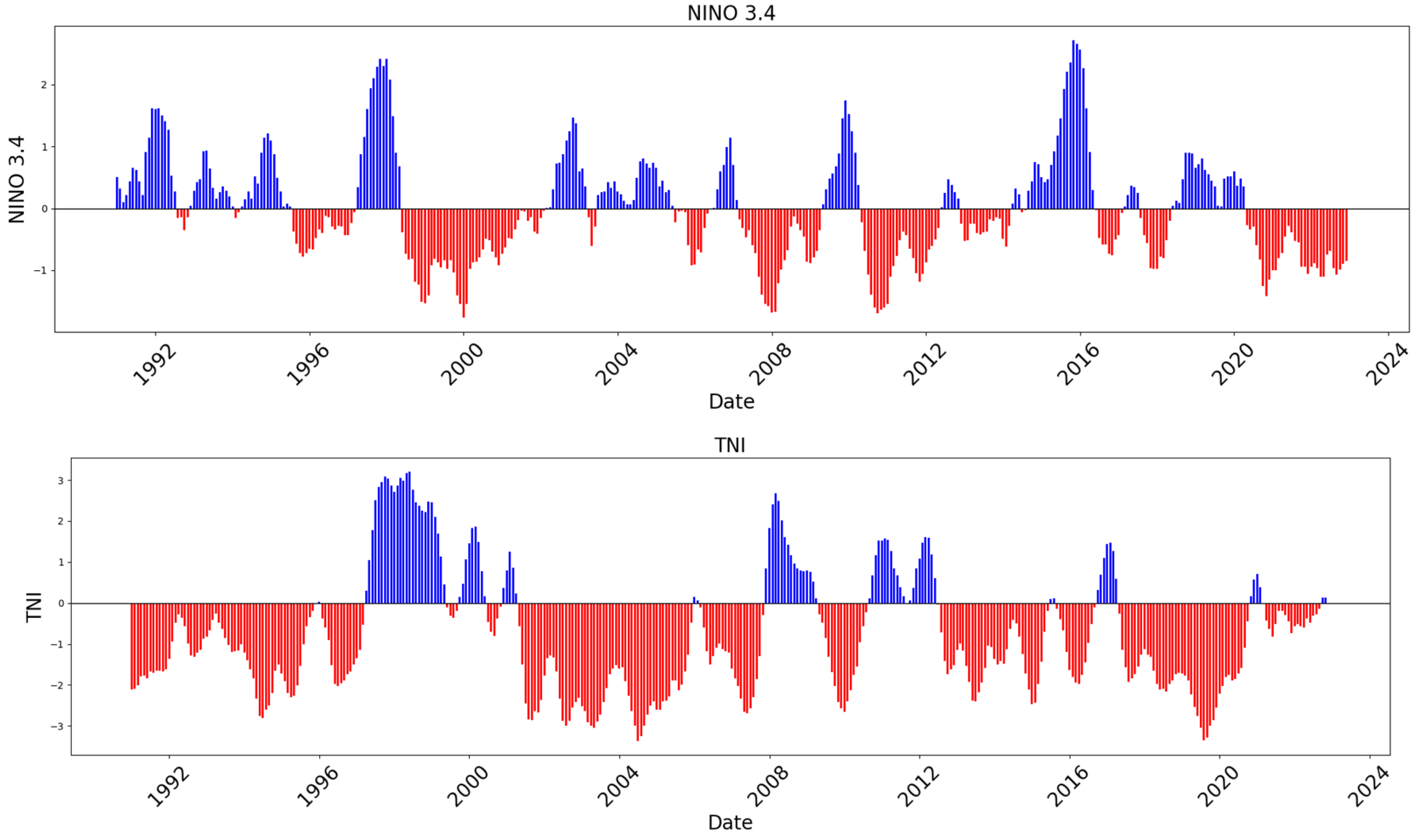
2.2.2. Climate Index

Climate represents the average atmospheric conditions that influence global weather phenomena over long periods, whereas weather refers to a short-term atmospheric state that changes frequently. Long-term climate change-driven changes have various impacts worldwide, including natural disasters, ecological changes, and social and economic losses. To analyze these climate changes, 15 climate indices were provided by the National Oceanic and Atmospheric Administration (NOAA): https://www.ncei.noaa.gov (accessed on 23 January 2024) [26]: AMO [27], AO [28], Heat Content [29], MEI [30], NAO [31], NINO3.4, NINO3, NINO4 [32], NP [33], OLR, ONI [34], PDO, PNA [35], SOI [36], and TNI [37], as shown in Figure 2.
This study compared and determined whether incorporating these climate indices into SPI-predicting models, which use only precipitation data, affects the model’s performance.

2.3. LSTM Algorithm

A Recurrent Neural Network (RNN) is a type of deep learning model that processes inputs and outputs in a sequence-based manner. RNNs are ANNs characterized by a cyclic structure wherein hidden nodes and edges are connected in a loop. The basic structure of an RNN is divided into three layers: hidden, input, and output.
The RNN demonstrated effectiveness when applied to relatively short sequences; however, issues with long-term dependencies arose as the sequence length increased. Specifically, as the sequence length increases, problems such as vanishing and exploding gradients occur during the backpropagation process, in which the gradients either diminish as they propagate back through the network or become excessively large, leading to unstable weight updates. To overcome these limitations, Hochreiter proposed the LSTM algorithm, which incorporates a cell-state structure into the hidden layers of traditional RNNs (Figure 3) [11].
f t = σ W f · h t 1 , x t + b i
i t = σ W i · h t 1 , x t + b i
C ~ t = tanh W c · h t 1 , x t + b c
C t = f t · C t 1 + i t · C ~ t
O t = σ W o · h t 1 , x t + b o
h t = O t · tanh C t
In this equation, f t represents the forget gate that determines the amount of information from the previous cell state C t 1 that should be discarded to address the long-term dependency issue and problems of vanishing and exploding gradients that exist in traditional RNNs. The forget gate is controlled by the weight matrix W f and the bias term b f . Then, the input gate i t updates the information from the current input x t and previous hidden state h t 1 , using the weight W i and bias term b i . The cell state is updated using C ~ t and C t , where C ~ t is computed based on the weight matrix W o and bias term b o . The hidden state h t is calculated using the output of the output gate and cell state, and this updated hidden state is used for learning in the current sequence.

Evaluation Metrics

The predictive performance of the LSTM algorithm was evaluated using standard regression evaluation metrics such as the MSE, RMSE, NSE, and coefficient of determination (R2). These standard regression evaluation metrics help understand the accuracy and predictive ability of deep and machine learning-based models.
M S E = 1 n i = 1 n ( y i y ^ i ) 2
  n : : S a m p l e   s i z e T o t a l   n u m b e r   o f   d a t a   p o i n t
  y i : : A c t u a l   o s e r v e d   v a l u e
  y ^ i : : P r e d i c t e d   v a l u e
The MSE represents the sum of the squared differences between the predicted and actual values averaged over the sample size. By squaring the differences, the MSE becomes sensitive to outliers. Hence, if large discrepancies occur between the predicted and actual values, the MSE value increases. The closer the MSE value is to 0, the better the prediction accuracy and performance of the model.
R M S E = 1 n i = 1 n ( y i y ^ i ) 2
  n : : S a m p l e   s i z e T o t a l   n u m b e r   o f   d a t a   p o i n t
  y i : : A c t u a l   o s e r v e d   v a l u e
  y ^ i : : P r e d i c t e d   v a l u e
RMSE is the square root of MSE. Although it has the same formulation as the MSE, it provides a more intuitive interpretation by expressing the error metric in a manner that is closer to the actual values. Similar to the MSE, the closer the RMSE value is to 0, the better the model performance, indicating that the predicted values are close to the actual values.
N S E = 1 y m t y i t 2 y i y ^ i 2
  y m t : : M e a n   o b s e r v e d   v a l u e
  y i : : A c t u a l   o b s e r v e d   v a l u e
  y ^ i : : P r e d i c t e d   v a l u e
The NSE is a statistical metric commonly used to evaluate the prediction performance of deep learning models in hydrology and meteorology. Its value ranges from negative to 1, where an NSE value is closer to 1, it suggests that the predicted values are similar to the actual values, thus confirming the strong predictive ability of the LSTM model.
R 2 = 1 i = 1 n ( y i y ^ i ) 2 i = 1 n ( y i y m t ) 2
  n : : S a m p l e   s i z e T o t a l   n u m b e r   o f   d a t a   p o i n t s
  y i : : A c t u a l   o b s e r v e d   v a l u e
  y ^ i : : P r e d i c t e d   v a l u e
  y m t : : M e a n   o b s e r v e d   v a l u e
R2 indicates how well the constructed model explains variability in the dependent variable. It ranges from 0 to 1, with values closer to 1 indicating that the model explains the variability of the dependent variable well, thereby verifying the accuracy of the model.
Using these evaluation metrics comprehensively, the performance of the scenario model built using meteorological and climate data to predict the actual SPI3 values was assessed. To construct a more sophisticated model, the parameters were adjusted, and meteorological and climate indices, as well as precipitation, were included. The results were derived by comparing standard regression evaluation metrics.

3. Results and Discussions

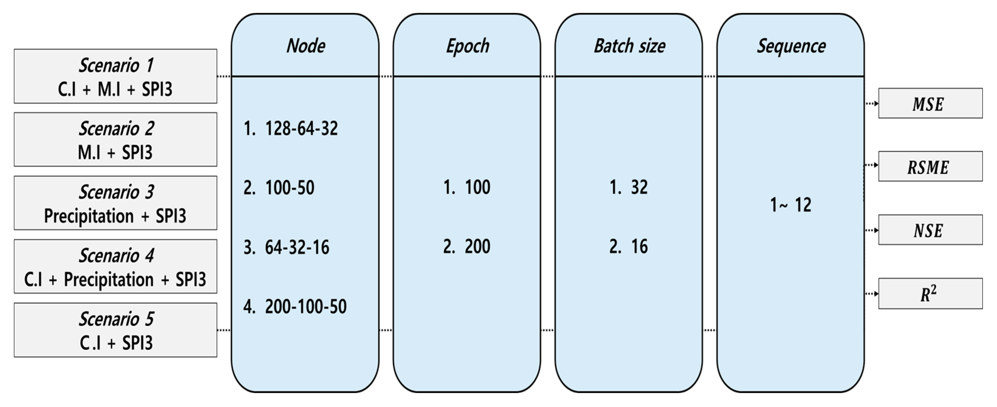
3.1. Algorithm Optimization

To predict the SPI using the LSTM algorithm, data, including the drought index SPI3, monthly precipitation, and meteorological and climatic indices, were used. Owing to the four different types of variables applied to the model, normalization was performed using a standard scalar. After normalization, 70% of the data were used for the training set and 30% for the test set, followed by a hyperparameter optimization process.
Various parameter combinations were applied to determine the optimal parameters for optimizing the performance of the LSTM prediction model. First, Adam was used as the optimizer, and Sigmoid and Tanh were applied as activation functions. Four nodes were set: 128-64-32, 100-50, 64-32-16, and 200-100-50. As monthly data were used, the sequence length, which represented the length of the input data, was set from 1 to 12. The batch sizes were set at 32 and 16, and the epochs representing the number of training iterations were set to 100 and 200, respectively. The hyperparameter optimization process was conducted using R2 as the primary evaluation metric. The parameter combination yielding the highest R2 value was selected as the optimal configuration. In addition, other evaluation metrics, including MSE, RMSE, and NSE, were calculated for comparison, and the final optimization was performed by considering these additional metrics to ensure the robustness of the selected model. For the target regions of Gwangju, Mokpo, Yeosu, and Jangheung, five scenarios were created to predict SPI: Scenario 1 used meteorological and climate indices with SPI3; Scenario 2 used meteorological indices and SPI3; Scenario 3 used monthly precipitation and SPI3; Scenario 4 used climate indices, monthly precipitation, and SPI3; and Scenario 5 used climate indices and SPI3.
Through this parameter adjustment process, this study aimed to find the optimal scenario for maximizing SPI prediction performance (Figure 4). The best scenario was identified by comparing the accuracy of five scenarios built with the optimized parameters using standard regression evaluation metrics.

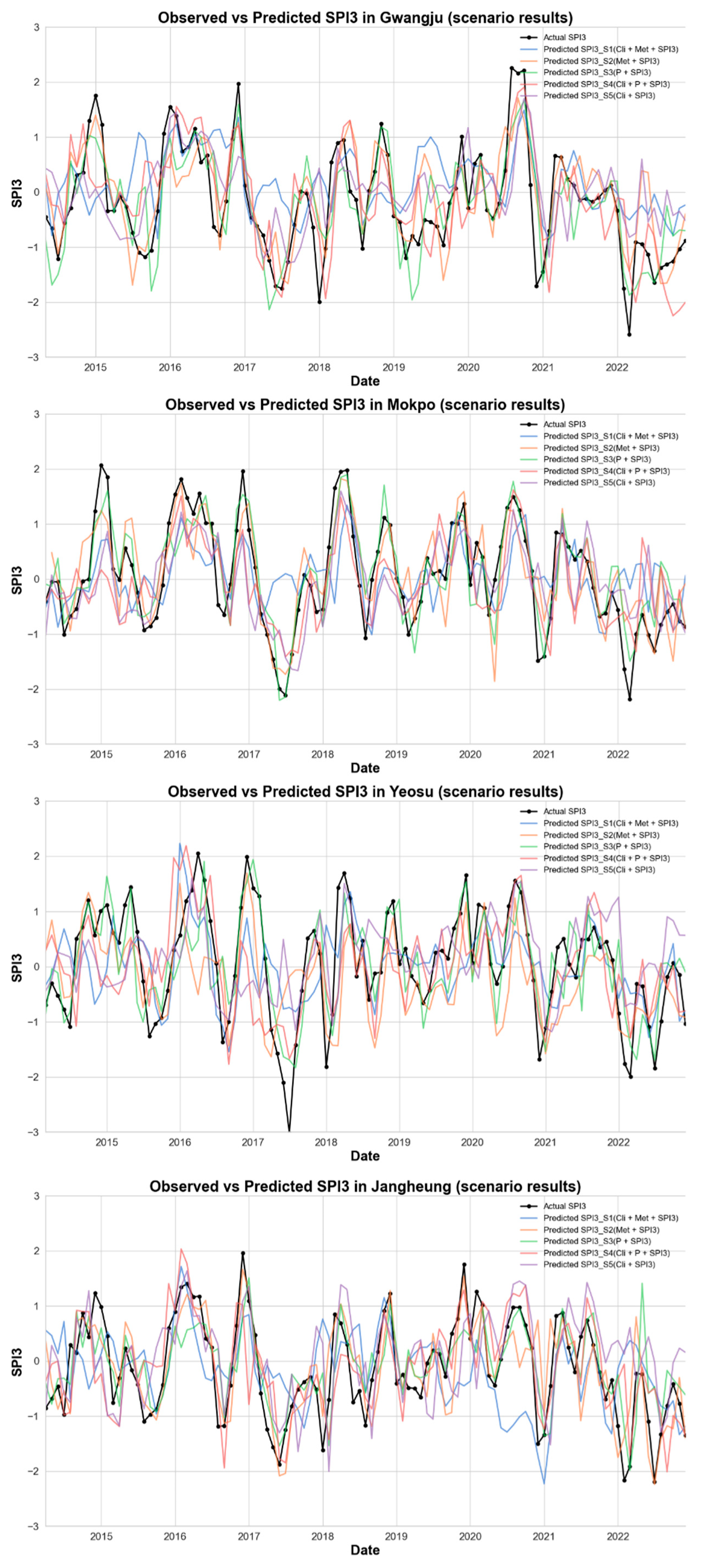
3.2. Drought Index Prediction

After hyperparameter optimization, the LSTM scenario with the optimal prediction performance was identified and visualized. Figure 5 shows that across all study regions, Scenario 3, which predicted the SPI3 using only precipitation, displayed a linear pattern similar to that of the original SPI3. Next in performance was Scenario 2, using meteorological indices, followed by Scenario 1, which combined climate and meteorological indices; Scenario 4, which used climate indices and precipitation; and Scenario 5, which predicted the SPI using only climate indices.
Table 2 lists the standard regression evaluation metrics. Scenario 3 predicted an MSE of 0.298, RMSE of 0.546, NSE of 0.579, and R2 of 0.675 for Gwangju (node: 64-32-16, batch size: 32, epoch: 100, sequence: 8); MSE of 0.200, RMSE of 0.477, NSE of 0.770, and R2 of 0.781 for Mokpo (node: 64-32-16, batch size: 16, epoch: 100, sequence: 5); MSE of 0.347, RMSE of 0.589, NSE of 0.628, and R2 of 0.647 for Yeosu (node: 128-64-32, batch size: 32, epoch: 100, sequence: 7); and MSE of 0.316, RMSE of 0.562, NSE of 0.578, and R2 of 0.580 for Jangheung (node: 100-50, batch size: 32, epoch: 100, sequence: 2). Consistent with the time-series linear graphs, Scenario 3 demonstrated the best performance.
A comparison of the SPI3 prediction performance across different scenarios using meteorological and climate indices along with precipitation data revealed that Scenario 3 exhibited the highest prediction accuracy. A similar finding was reported by Hassanzadeh et al. (2020) [38], who found that precipitation and humidity played dominant roles in SPI predictions. Their study, which applied ANNs to forecast SPI in Iran, concluded that precipitation had the highest impact on prediction accuracy, whereas sunshine hours contributed the least. This consistency suggests that precipitation-driven models effectively enhanced drought prediction accuracy across different geographical regions. Additionally, our study found that Scenario 5 had the lowest prediction performance, indicating that climate change may not be directly correlated with short-term SPI variations. However, as Hassanzadeh et al. (2020) [38] did not incorporate climate indices into their study, direct comparisons were limited. However, climate indices are indicators that reflect long-term atmospheric–oceanic interactions, and therefore, they may not have been suitable for short-term drought predictions like SPI. On the other hand, recent studies, such as Yalçın et al. (2023) [39], have demonstrated that hybrid models like CNN-LSTM, which combine CNN and LSTM, can significantly improve prediction performance. Using various station locations, time scales, and estimators, they predicted SPEI6 and SPEI9, achieving RMSE of 0.72, MADE of 0.35, MAE of 0.22, and R2 of 99.53%, outperforming existing machine learning and deep learning techniques. This suggests that combining CNN with LSTM can effectively capture both spatial and temporal dependencies, leading to improved drought prediction accuracy.
Therefore, future research should focus on analyzing potential improvements in prediction performance when combining climate and meteorological indices alongside advanced deep learning models. While the standalone use of climate indices in this study did not significantly enhance the prediction accuracy, this could be due to the nature of climate indices, which capture long-term atmospheric–oceanic interactions. Consequently, exploring the combined use of climate indices, meteorological indices, and deep learning hybrid models such as CNN-LSTM is expected to improve both short- and long-term drought prediction accuracy. Hybrid models like CNN-LSTM, which effectively capture both spatial and temporal dependencies, have demonstrated their ability to outperform traditional methods and enhance prediction reliability. Thus, future work should integrate these approaches to develop more robust models for drought prediction across various timescales and geographical regions.

3.3. Prediction Results of Seasonal Variability of SPI

Based on the four distinct seasons observed in South Korea, the monthly meteorological, climate indices, and SPI3 were divided into spring (March–May), summer (June–August), fall (September–November), and winter (December–February). For seasonal evaluation, standard regression performance indicators were conducted, focusing on Mokpo, the target region, using Scenario 3, as it showed the best performance in calculating SPI3 using only precipitation data.
Table 3 examines the seasonal regression performance indicators for Mokpo in Scenario 3. In fall (September–November), although the NSE and R2 values were lower than those in winter, the MSE and RMSE values were closer to 0, indicating better performance. While the MSE, NSE, and R2 values of spring were not as high as those in winter, it still showed a relatively good overall performance, with a slightly lower performance compared to that of fall. While the NSE and R2 values of summer were the lowest, its MSE and RMSE values were similar, though slightly better than those of winter.
Extending SPI timescales improves prediction accuracy due to the reduction of short-term fluctuations in SPI at larger timescales, as noted in previous research [38]. In that study, longer SPI timescales exhibited more stable trends, making it easier for machine learning models to capture patterns effectively. Similarly, our study found that seasonal SPI predictions in winter were the most stable, likely because winter exhibits lower short-term variability in precipitation than other seasons. This contributed to a more consistent trend in SPI3, thereby enhancing the LSTM prediction accuracy. The similarity between these findings suggests that increasing SPI timescales and considering seasonal characteristics may help improve drought prediction performance by minimizing short-term variations that can introduce uncertainty.

4. Conclusions

In this study, to assess the impact on drought index prediction, we utilized the SPI3 and meteorological indices from the ASOS, as well as climate indices provided by NOAA for the Yeongsan and Seomjin River basins in South Korea, which have recently suffered severe drought damage. Data from four regions (Gwangju, Mokpo, Yeosu, and Jangheung) were preprocessed, and five LSTM scenarios were constructed. These were divided into training and test sets for model development and were evaluated using standard regression performance metrics. This study focused on four regions in the study area and collected monthly data on meteorological indices and SPI3 from 1991 to 2022, including monthly climate indices provided by the NOAA and Atmospheric Administration. The data was preprocessed and applied to the LSTM model. The training set was 70%, the test set was 30%, and the LSTM model was trained using various combinations of hyperparameters. A hyperparameter optimization process was conducted to determine the optimal combination that maximized the prediction performance. The optimized parameters included the optimizer, activation functions, number of nodes, sequence length, batch size, and number of epochs. Hyperparameter optimization aimed to maximize the R2 value, whereas other evaluation metrics, such as MSE, RMSE, and NSE, were also considered for the final model selection.
The analysis revealed that Scenario 3 demonstrated the highest performance based on standard regression metrics. The Mokpo station, which recorded the best performance among the study regions, achieved an MSE of 0.200, RMSE of 0.477, NSE of 0.770, and R2 of 0.781. The performances decreased in the following order: Scenario 2 (meteorological indices and SPI3), Scenario 1 (combining meteorological and climate indices with SPI3), Scenario 4 (climate indices, precipitation, and SPI3), and Scenario 5 (climate indices and SPI3). When climate indices were included, the decrease in performance was attributed to the SPI calculation method, which relies solely on precipitation. Climate indices, which reflect relatively long-term variability, may have limited correlation with short-term SPI fluctuations, thereby contributing less to the prediction performance. The seasonal applicability of Scenario 3 was also evaluated considering South Korea’s distinct four-season climate. The data were divided into spring (March–May), summer (June–August), fall (September–November), and winter (December–February), and seasonal standard regression performance metrics were analyzed. Winter exhibited the highest prediction performance, with average values of 0.367, 0.606, 0.702, and 0.702, respectively. This result is attributed to the relatively low short-term variability of precipitation during winter, which allows for a more consistent SPI3 trend, thus improving prediction accuracy.
This study assessed the applicability of drought index prediction models using LSTM with various meteorological and climatic indices. Therefore, Scenario 3 showed the highest performance. Although scenarios incorporating climate indices demonstrated relatively lower performances, climate indices were determined to have some impact. This suggests that climate indices that reflect long-term atmospheric–oceanic interactions may play a critical role in long-term drought pattern analysis and climate change-related drought predictions, although their contribution to short-term SPI predictions may be limited. Therefore, future research should focus on developing methods to effectively incorporate the long-term characteristics of climate indices, integrate topographic data (such as DEM, slope, and aspect), and apply various deep and machine learning models to improve the accuracy of both short- and long-term drought predictions.

Author Contributions

Conceptualization, S.P. and H.H.; methodology, S.P. and H.H.; software, S.P.; validation, S.P.; formal analysis, S.P.; investigation, S.P. and H.H.; data curation, S.P.; writ-ing—original draft preparation, S.P.; writing—review and editing, S.P. and H.H.; visualization, S.P. and H.H.; supervision, H.H.; project administration, H.H.; funding acquisition, H.H. All authors have read and agreed to the published version of the manuscript.

Funding

This work was supported by the National Research Foundation of Korea (NRF) grant funded by the Korea government (MSIT) (No. RS-2023-00243413).

Data Availability Statement

The data will be available upon request to the corresponding author.

Conflicts of Interest

The authors declare no conflicts of interest.

References

  1. Zittis, G.; Hadjinicolaou, P.; Lelieveld, J. Role of soil moisture in the amplification of climate warming in the eastern Mediterranean and the Middle East. Clim. Res. 2014, 59, 27–37. [Google Scholar] [CrossRef]
  2. Samuel, A.L. Some studies in machine learning using the game of checkers. IBM J. Res. Dev. 1959, 3, 210–229. [Google Scholar] [CrossRef]
  3. McCulloch, W.S.; Pitts, W. A logical calculus of the ideas immanent in nervous activity. Bull. Math. Biol. 1943, 5, 115–133. [Google Scholar] [CrossRef]
  4. Langley, P.; Iba, W.; Thompson, K. An analysis of Bayesian classifiers. In Proceedings of the AAAI’92: Proceedings of the Tenth National Conference on Artificial Intelligence, San Jose, CA, USA, 12–16 July 1992; Volume 90, pp. 223–228. [Google Scholar]
  5. Breiman, L. Random forests. Mach. Learn. 2001, 45, 5–32. [Google Scholar] [CrossRef]
  6. Hearst, M.A.; Dumais, S.T.; Osuna, E.; Platt, J.; Scholkopf, B. Support vector machines. IEEE Intell. Syst. Appl. 1998, 13, 18–28. [Google Scholar] [CrossRef]
  7. Lee, D.D.; Seung, H.S. Learning the parts of objects by non-negative matrix factorization. Nature 1999, 401, 788–791. [Google Scholar] [CrossRef]
  8. Johnson, S.C. Hierarchical clustering schemes. Psychometrika 1967, 32, 241–254. [Google Scholar] [CrossRef]
  9. McInnes, L.; Healy, J.; Melville, J. Umap: Uniform manifold approximation and projection for dimension reduction. arXiv 2018, arXiv:1802.03426. [Google Scholar] [CrossRef]
  10. Lloyd, S. Least squares quantization in PCM. IEEE Trans. Inf. Theory 1982, 28, 129–137. [Google Scholar] [CrossRef]
  11. Hochreiter, S.; Schmidhuber, J. Long short-term memory. Neural Comput. 1997, 9, 1735–1780. [Google Scholar] [CrossRef]
  12. Feng, P.; Wang, B.; Li Liu, D.; Yu, Q. Machine learning-based integration of remotely-sensed drought factors can improve the estimation of agricultural drought in South-Eastern Australia. Agric. Syst. 2019, 173, 303–316. [Google Scholar] [CrossRef]
  13. Rahmati, O.; Falah, F.; Dayal, K.S.; Deo, R.C.; Mohammadi, F.; Biggs, T.; Bui, D.T. Machine learning approaches for spatial modeling of agricultural droughts in the south-east region of Queensland Australia. Sci. Total Environ. 2020, 699, 134230. [Google Scholar] [CrossRef] [PubMed]
  14. Tyagi, S.; Zhang, X.; Saraswat, D.; Sahany, S.; Mishra, S.K.; Niyogi, D. Flash drought: Review of concept, prediction and the potential for machine learning, deep learning methods. Earth’s Future 2022, 10, e2022EF002723. [Google Scholar] [CrossRef]
  15. Mokhtar, A.; Jalali, M.; He, H.; Al-Ansari, N.; Elbeltagi, A.; Alsafadi, K.; Rodrigo-Comino, J. Estimation of SPEI meteorological drought using machine learning algorithms. IEEE Access 2021, 9, 65503–65523. [Google Scholar] [CrossRef]
  16. Zhang, R.; Chen, Z.Y.; Xu, L.J.; Ou, C.Q. Meteorological drought forecasting based on a statistical model with machine learning techniques in Shaanxi province, China. Sci. Total Environ. 2019, 665, 338–346. [Google Scholar] [CrossRef]
  17. Karbasi, M.; Jamei, M.; Malik, A.; Kisi, O.; Yaseen, Z.M. Multi-steps drought forecasting in arid and humid climate environments: Development of integrative machine learning model. Agric. Water Manag. 2023, 281, 108210. [Google Scholar] [CrossRef]
  18. IPCC. Summary for Policymakers. In Climate Change 2013: The Physical Science Basis, Contribution of Working Group I to the Fifth Assessment Report of the Intergovernmental Panel on Climate Change; Stocker, T.F., Qin, D., Plattner, G.-K., Tignor, M., Allen, S.K., Boschung, J., Nauels, A., Xia, Y., Bex, V., Midgley, P.M., Eds.; Cambridge University Press: Cambridge, UK, 2013; p. 15. [Google Scholar]
  19. Shamshirband, S.; Hashemi, S.; Salimi, H.; Samadianfard, S.; Asadi, E.; Shadkani, S.; Chau, K.W. Predicting standardized streamflow index for hydrological drought using machine learning models. Eng. Appl. Comput. Fluid Mech. 2020, 14, 339–350. [Google Scholar] [CrossRef]
  20. Belayneh, A.; Adamowski, J. Drought forecasting using new machine learning methods. J. Water Land Dev. 2013, 18, 3–12. [Google Scholar] [CrossRef]
  21. Kim, C.; Kim, C.S. Comparison of the performance of a hydrologic model and a deep learning technique for rainfall-runoff analysis. Trop. Cyclone Res. Rev. 2021, 10, 215–222. [Google Scholar] [CrossRef]
  22. K-water. Drought White Paper on the Yeongsan & Sumjin River Basin (2022–2023); K-water: Daejeon, Republic of Korea, 2023; p. 139. [Google Scholar]
  23. Korea Meteorological Administration (KMA). Precipitation Data. Available online: https://data.kma.go.kr (accessed on 23 January 2024).
  24. McKee, T.B.; Doesken, N.J.; Kleist, J. The relationship of drought frequency and duration to time scales. In Proceedings of the 8th Conference on Applied Climatology, Anaheim, CA, USA, 17–22 January 1993; Volume 17, pp. 179–183. [Google Scholar]
  25. Kim, G.S.; Lee, J.W. Evaluation of drought indices using drought records. J. Korea Water Resour. Assoc. 2011, 44, 639–652. [Google Scholar] [CrossRef]
  26. National Oceanic and Atmospheric Administration (NOAA). Climate Indices. Available online: https://www.ncei.noaa.gov (accessed on 23 January 2024).
  27. Nye, J.A.; Baker, M.R.; Bell, R.; Kenny, A.; Kilbourne, K.H.; Friedland, K.D.; Wood, R. Ecosystem effects of the Atlantic multidecadal oscillation. J. Mar. Syst. 2014, 133, 103–116. [Google Scholar] [CrossRef]
  28. Rigor, I.G.; Wallace, J.M.; Colony, R.L. Response of sea ice to the Arctic Oscillation. J. Clim. 2002, 15, 2648–2663. [Google Scholar] [CrossRef]
  29. Yu, J.Y.; Kao, H.Y. Decadal changes of ENSO persistence barrier in SST and ocean heat content indices: 1958–2001. J. Geophys. Res. Atmos. 2007, 112, 13106. [Google Scholar] [CrossRef]
  30. Wolter, K.; Timlin, M.S. El Niño/Southern Oscillation behaviour since 1871 as diagnosed in an extended multivariate ENSO index (MEI. ext). Int. J. Climatol. 2011, 31, 1074–1087. [Google Scholar] [CrossRef]
  31. Stenseth, N.C.; Ottersen, G.; Hurrell, J.W.; Mysterud, A.; Lima, M.; Chan, K.S.; Ådlandsvik, B. Studying climate effects on ecology through the use of climate indices: The North Atlantic Oscillation, El Nino Southern Oscillation and beyond. Proc. Biol. Sci. 2003, 270, 2087–2096. [Google Scholar] [CrossRef]
  32. Trenberth, K.E.; Stepaniak, D.P. Indices of el Niño evolution. J. Clim. 2001, 14, 1697–1701. [Google Scholar] [CrossRef]
  33. Linkin, M.E.; Nigam, S. The North Pacific Oscillation–west Pacific teleconnection pattern: Mature-phase structure and winter impacts. J. Clim. 2008, 21, 1979–1997. [Google Scholar] [CrossRef]
  34. Glantz, M.H.; Ramirez, I.J. Reviewing the Oceanic Niño Index (ONI) to enhance societal readiness for El Niño’s impacts. Int. J. Disaster Risk Sci. 2020, 11, 394–403. [Google Scholar] [CrossRef]
  35. Ge, Y.; Luo, D. Impacts of the different types of El Niño and PDO on the winter sub-seasonal North American zonal temperature dipole via the variability of positive PNA events. Clim. Dyn. 2023, 60, 1397–1413. [Google Scholar] [CrossRef]
  36. Kwok, R.; Comiso, J.C. Southern Ocean climate and sea ice anomalies associated with the Southern Oscillation. J. Clim. 2002, 15, 487–501. [Google Scholar] [CrossRef]
  37. Trenberth, K.E.; Shea, D.J. Atlantic hurricanes and natural variability in 2005. Geophys. Res. Lett. 2006, 33, 12704. [Google Scholar] [CrossRef]
  38. Hassanzadeh, Y.; Ghazvinian, M.; Abdi, A.; Baharvand, S.; Jozaghi, A. Prediction of short and long-term droughts using artificial neural networks and hydro-meteorological variables. arXiv 2020, arXiv:2006.02581. [Google Scholar] [CrossRef]
  39. Yalçın, S.; Eşit, M.; Çoban, Ö. A new deep learning method for meteorological drought estimation based-on standard precipitation evapotranspiration index. Eng. Appl. Artif. Intell. 2023, 124, 106550. [Google Scholar] [CrossRef]
Figure 1. Study area: (A) Yeongsan and SeomJin River Basins, (B) Gwangju, (C) Mokpo, (D) Jangheung, (E) Yeosu (regions (BD) are included in the Yeongsan River Basin, whereas region (E) is included in the Seomjin River Basin).
Water 17 01801 g001
Figure 2. Time series of climate indices (AMO, AO, NINO 3.4, TNI) from 1991 to 2022.
Water 17 01801 g002aWater 17 01801 g002b
Figure 3. Structure of Long Short-Term Memory algorithm.
Water 17 01801 g003
Figure 4. LSTM hyperparameter optimization (C.I = climate index, M.I = meteorological index).
Water 17 01801 g004
Figure 5. Time series of scenario-based prediction results using the LSTM algorithm.
Water 17 01801 g005
Table 1. List of meteorological data collected from the Automated Synoptic Observing System.
Meteorological DataDate (Resolution)Sources
Average temperature1991–2022 (Monthly)KMA
Average local atmospheric pressure1991–2022 (Monthly)KMA
Average sea-surface atmospheric pressure1991–2022 (Monthly)KMA
Average water vapor pressure1991–2022 (Monthly)KMA
Average dew point temperature1991–2022 (Monthly)KMA
Average relative humidity1991–2022 (Monthly)KMA
Total precipitation per month1991–2022 (Monthly)KMA
Average wind speed1991–2022 (Monthly)KMA
Total daily flow1991–2022 (Monthly)KMA
Average cloudiness1991–2022 (Monthly)KMA
Average ground temperature1991–2022 (Monthly)KMA
Sunshine rate1991–2022 (Monthly)KMA
Table 2. Evaluation results of the five scenarios.
Scenario 1
StationsNodesBatch sizeEpochsSequenceMSERMSENSE R 2
Gwangju100-5016100120.4420.6650.1430.529
Mokpo128-64-3216200110.2770.5260.3990.709
Yeosu200-100-5016200100.4300.6560.3220.570
Jangheung200-100-5016100110.3580.5980.2630.533
Scenario 2
StationsNodesBatch sizeEpochsSequenceMSERMSENSE R 2
Gwangju128-64-321610070.2740.5230.5430.699
Mokpo64-32-1616100120.2290.4790.4250.760
Yeosu200-100-501610070.3740.6120.2550.620
Jangheung64-32-163210020.3540.5950.5280.530
Scenario 3
StationsNodesBatch sizeEpochsSequenceMSERMSENSE R 2
Gwangju64-32-163210080.2980.5460.5790.675
Mokpo64-32-161610050.2000.4470.7700.781
Yeosu128-64-323210070.3470.5890.6280.647
Jangheung100-503210020.3160.5620.5780.580
Scenario 4
StationsNodesBatch sizeEpochsSequenceMSERMSENSE R 2
Gwangju200-100-501620020.5340.7310.3310.356
Mokpo128-64-321620040.4070.6380.4730.551
Yeosu64-32-161610020.5700.7550.2970.406
Jangheung100-501610020.4510.6710.3420.401
Scenario 5
StationsNodesBatch sizeEpochsSequenceMSERMSENSE R 2
Gwangju128-64-323220050.6170.7860.1490.309
Mokpo200-100-503210050.5210.7220.3600.430
Yeosu100-503210090.6950.8340.0490.303
Jangheung200-100-501620020.6950.8330.0670.077
Table 3. Seasonal prediction results in Mokpo (Scenario 3).
StationSeasonsMSERMSENSE R 2
MokpoSpring0.2810.5300.6380.638
Summer0.3650.6040.4930.493
Fall0.2560.5060.6780.678
Winter0.3670.6060.7020.702
Disclaimer/Publisher’s Note: The statements, opinions and data contained in all publications are solely those of the individual author(s) and contributor(s) and not of MDPI and/or the editor(s). MDPI and/or the editor(s) disclaim responsibility for any injury to people or property resulting from any ideas, methods, instructions or products referred to in the content.

