Statistical and Physical Significance of Homogeneous Regions in Regional Flood Frequency Analysis

Abstract

This study investigates formation homogeneous regions in regional flood frequency analysis (RFFA) and compares two RFFA methods, the quantile regression technique (QRT) and the index flood method (IFM). A total of 201 gauged stations from southeast Australia were adopted in this study. Multivariate statistical techniques were applied to form candidate regions. Also, regions are formed in the L-moments space (such as the L coefficient of variation (LCV) and L coefficient of skewness (LCS) of annual maximum flood data). Hosking and Wallis test statistics were used to find discordant sites and for testing the homogeneity of the assumed regions. No homogeneous regions were found in southeast Australia based on catchment characteristics data; however, homogeneous regions can be formed in the space of L-moments. It was found that regions formed in the L-moments space have little link with the catchment characteristics data space. The QRT provides more accurate flood quantile estimates than the IFM.

1. Introduction

Floods are a natural disaster that cause significant loss to the economy and livelihoods [1,2,3]. In the USA, floods account for more than 75 percent of US federal disaster declarations [4]. Flood risk assessment is essential [5] to minimize flood damage, and in this regard, design flood estimation is widely used in risk-based planning and design [6,7,8,9]. Design flood estimation is widely used in the design of hydraulic structures [10], floodplain management, and water resource planning [11] studies.

In design flood estimation at a given location, recorded flood data of sufficient length and good quality are needed. However, at many locations of interest, recorded flood data are either non-existent or of limited length or of poor quality. In these cases, regional flood frequency analysis (RFFA) is adopted, which aims to transfer flood characteristics from a homogeneous region to an ungauged location [12,13,14].

The index-flood method (IFM) is widely used in RFFA [15]. The IFM assumes that flood distributions within a homogeneous region differ only by a scaling factor. The L-moments-based IFM has become quite popular in RFFA as L-moments provide more accurate estimation of distributional parameters than the ordinary product moments [16]. The parameter regression technique (PRT) and quantile regression technique (QRT) are also widely used in RFFA, which are not strictly dependent on the homogeneity assumption [17,18].

In RFFA, one of the most challenging steps is to identify homogeneous regions [19]. Regions in RFFA are generally formed in two ways: (a) fixed regions—where regions are formed based on geographic boundary; and (b) the region of influence (ROI) approach—where a local region is formed either in the catchment data space or in a geographical space [20].

There are statistical methods to test the degree of homogeneity of a hypothesized region [16,21]. These tests have been widely adopted in RFFA. However, there are cases where perfect homogeneous regions cannot be established, e.g., in Australia, the attempts to form homogeneous regions were not successful [22,23,24,25]. There have been limited studies on the physical significance (e.g., geographical contiguity) of homogeneous regions. To fill this knowledge gap, this study aims to answer the following questions: (i) Whether regions formed based on catchment area and drainage division deliver homogeneous regions in southeast Australia? (ii) Whether regions formed in the space of flood characteristics have meaningful linkage with catchment characteristics? (iii) In a heterogeneous region like southeast Australia, whether regression-based RFFA techniques (such as QRT) are preferable to the IFM?

This study forms regions in several ways, i.e., (i) regions based on catchment size; (ii) regions based on drainage divisions; (iii) regions based on basin proximity; and (iv) regions based on the L-moments space. The regions formed in the L-moments space are linked with the catchment characteristics data space and geographical space. Furthermore, this study compares two RFFA methods, the QRT (where the homogeneity assumption is relaxed) and the IFM (where the homogeneity of a region is a prerequisite).

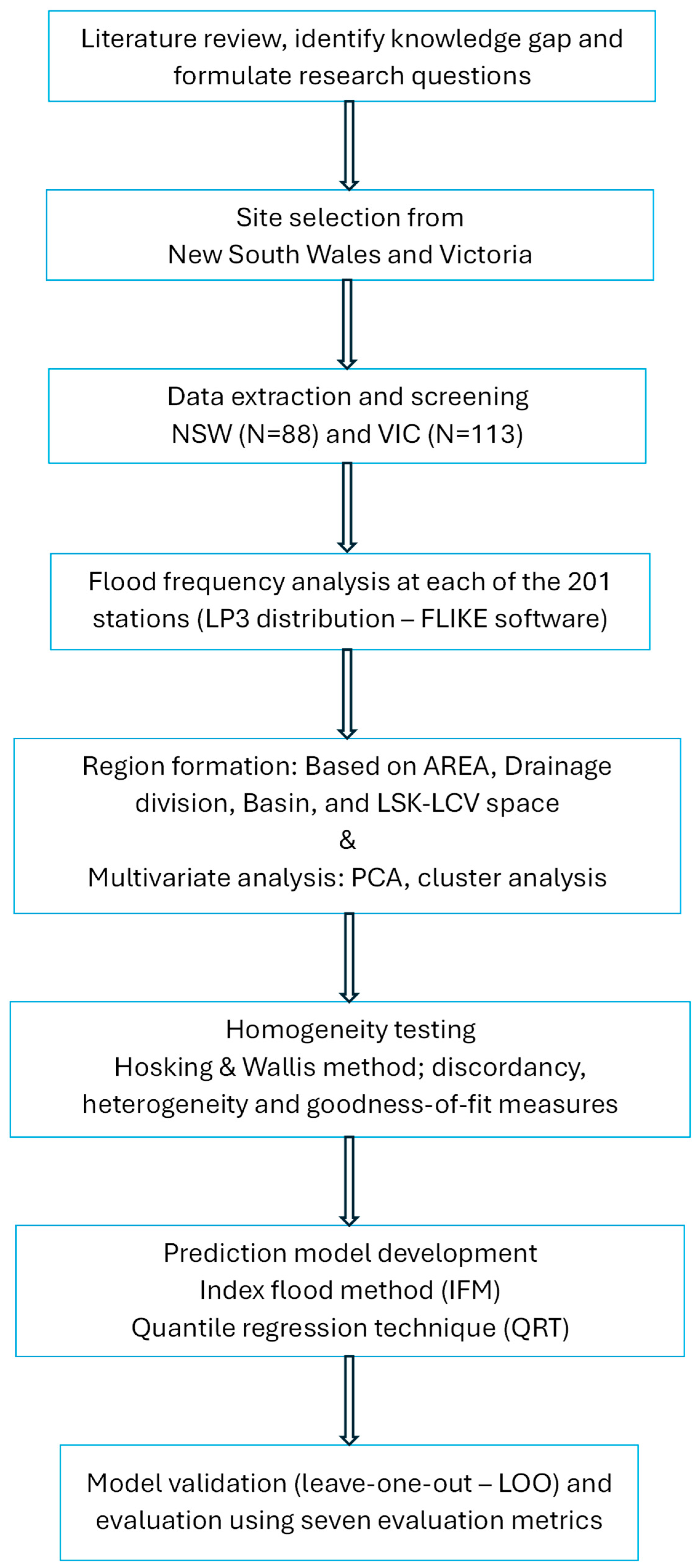
2. Data and Methodology

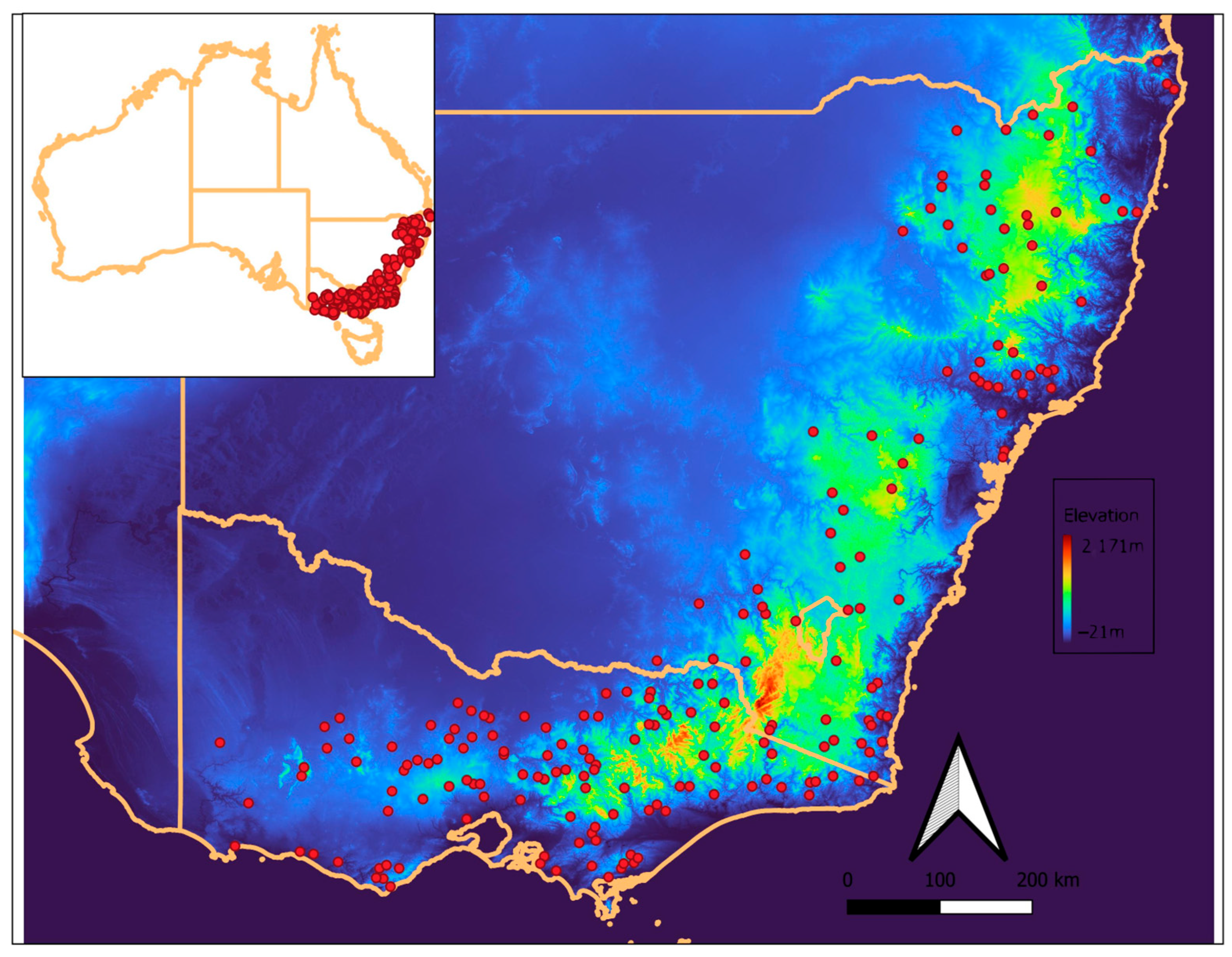
The adopted methodology is illustrated in Figure 1.

2.1. Study Area

The States of New South Wales (NSW) and Victoria (VIC) in the southeast part of Australia were selected as the study area. A total of 201 gauged stations were selected in this study, as shown in Figure 2. The reason for selecting this part of Australia is that this has better quality streamflow data as compared to other parts of Australia [23,24]. The selected catchments are predominantly natural and are not subject to any major urbanization and artificial storage [22,25]. Geographically, these catchments lie within the range from latitudes −38.76° to −28.36° south and longitudes from 141.47° to 153.50° east. This area is dominated by highly variable hydrology and various climates such as cool, hot, dry, humid, arid, and semi-arid. Bates et al. [22] suggested that the weather of the study region is controlled by an extratropical high-pressure system from west-to-east, which generates heavy rainfalls and thunderstorms. The Murray–Darling and South-East Coast divides the study area into two main drainage divisions by vast ridges of mountain relief. It is known as the Great Dividing Range (GDR). Coastal areas are separated from the plain inland areas by this GDR. The Snowy Mountain regions and the Victorian Alps, the highest mountains in the Australian mainland, are the part of the GDR and fall in our study area.

2.2. Exploratory Data Analysis

Based on the recommendations for catchment selection criteria [26,27], this study used eight catchment and climatic characteristics as predictor variables. These are: (i) catchment area (AREA, km²), (ii) design rainfall intensity with duration of 6 h and 1 in 2 AEP (I₆₂, mm/h), (iii) mean annual rainfall (MAR, mm), (iv) shape factor (SF), (v) mean annual evapotranspiration (MAE, mm), (vi) stream density (SDEN, km⁻¹), (vii) slope of central 75% of mainstream (S1085, m/km), and (viii) fraction of area forested (FOREST, fraction). The predictor variables data were obtained from the Australian Bureau of Meteorology (BoM) website and Australian Rainfall and Runoff Revision Project 5 Regional flood methods [28]. Many Australian RFFA studies also adopted most of these predictors [22,25,27,29,30,31].

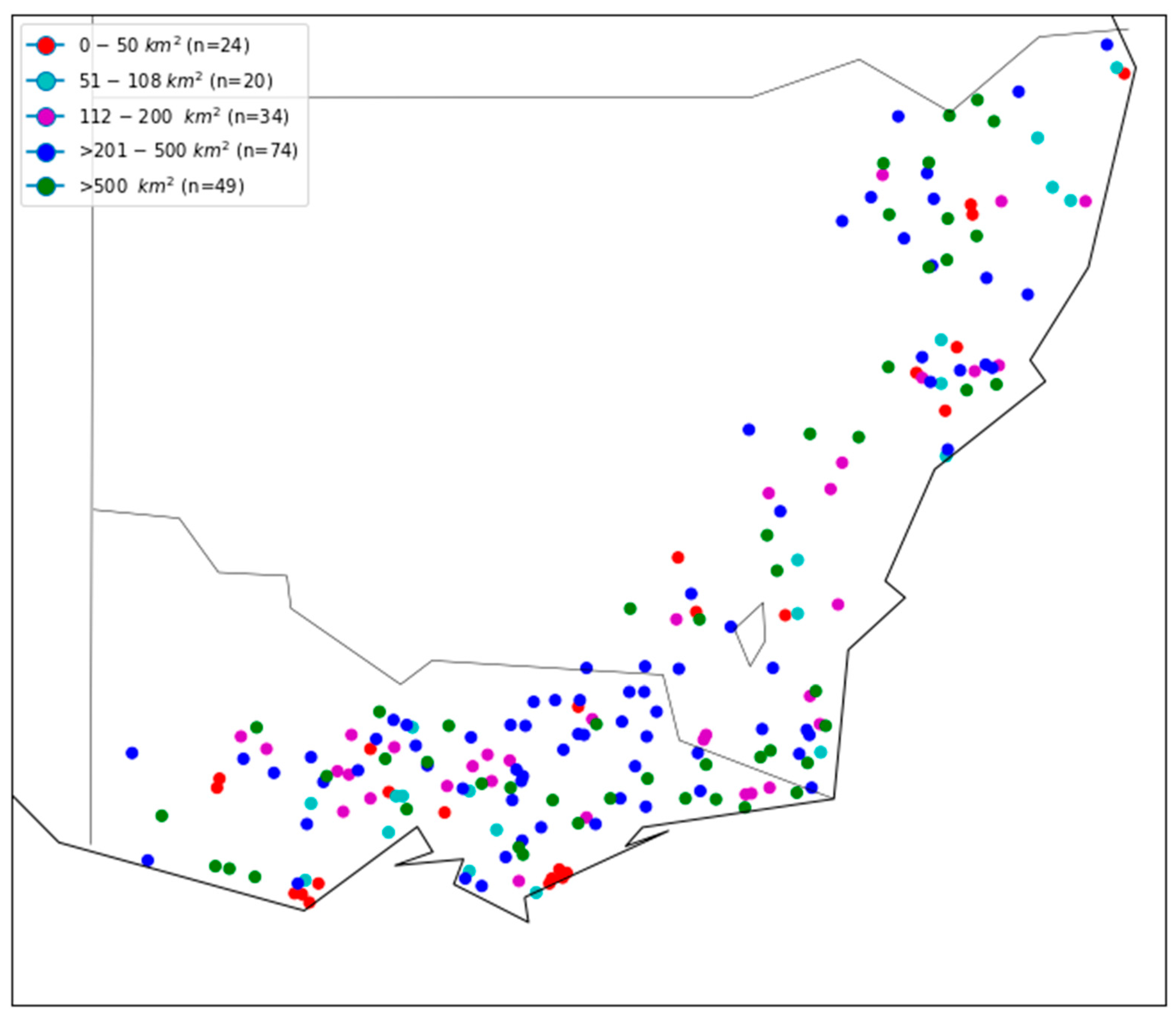
Catchment and Climate Characteristics

The value of the catchment area (AREA) ranges from 3.00 to 1010.00 km² with a mean of 333.99 km² and standard deviation (SD) of 262.40 km². Only one station has an AREA of 1010 km², but the majority of them are below 400 km² (n = 138, ~69%). The shape factor (SF) values lie between 0.26 and 1.63 (mean ± SD; 0.78 ± 0.21) with a median of 0.78. The mean and median values of stream density (SDEN) of the selected catchments are 2.10 km⁻¹ and 1.69 km⁻¹, respectively (SD = 1.06 km⁻¹). Similarly, these figures for mainstream slope (S1085) are 13.19 m/km, 9.50 m/km, and SD = 11.67 m/km, respectively. The values for the forest fraction (FOREST) vary from 0 to 1 with a mean of 0.55 and the median is 0.59 (SD = 0.34).

With a range of 25 to 89 years (mean ± SD; 45 ± 9.63), the record length of streamflow data for majority of stations (n = 137, ~68%) lies between 40 to 50 years. Additional summary statistics for assumed regions can be found in Figure 3 (including the L-moments of annual maximum (AM) flood data; L-coefficient of variation (LCV); and L-coefficient of skewness (LSK)) and in the Supplementary Section (see Table S1).

Data for the rainfall intensity of 6 h duration in 1 in 2 AEP (I₆₂) and the mean annual evapotranspiration (MAE) were extracted from the Australian Bureau of Meteorology (BoM) website. The value of I₆₂ ranges from 24.60 to 87.30 mm/h with a median of 37.30 mm/h (mean ± SD; 39.16 ± 10.07 mm/h). The maximum and the minimum values for the predictor MAR are 484.39 mm and 1953.23 mm (mean ± SD; 962.26 ± 314.47 mm), respectively. For MAE, these figures are 1543.30, 925.90, and 1117.96 ± 129.31 mm, respectively. Region-specific summary statistics of predictor variables are explained in Section 3.5.

2.3. Formation of Regions and Testing for Homogeneity

2.3.1. Homogeneous Region Identification

In the identification of homogeneous regions, a fixed region approach was applied in different ways. Firstly, based on the categorization of AREA the selected stations were divided into five groups. These are G-A1 (0 to 50 km²), G-A2 (51 to 108 km²), G-A3 (112 to 200 km²), G-A4 (>200 to 500 km²), and G-A5 (>500 km²). Figure 3 shows the spatial distribution of 201 stations by their AREA category. Secondly, considering the drainage division (DD), two groups were formed. Group 1 (G-D1) consists of the stations, starting the DD number with “2”, and group 2 (G-D2) starts with “4”. Again, based on these two groups, “States” were considered and 2 groups were formed for each. Under the DD “2”, the two groups are G-D3 (within NSW) and G-D4 (within VIC) and for DD “4”, these two groups are G-D5 (within NSW) and G-D6 (within VIC). In addition, based the north and south part of NSW within DD “2” another two regions were formed (G-D7 and G-D8). Similarly, based on the eastern and western part of VIC and DD “2”, the formed regions are G-D9 and G-D10. Adopting the same approach for DD “4”, four regions were formed, which are G-D11, G-D12, G-D13, and G-D14, respectively. Thirdly, considering the neighborhood basins, eight groups were formed: G-B1, G-B2, G-B3, G-B4, G-B5, G-B6, G-B7, and G-B8. Finally, the LCV and LSK space was split to form the following regions: the (a) single largest homogeneous region (G-LMA), (b) two largest homogeneous regions (G-LMB1 and G-LMB2), (c) three largest homogeneous regions (G-LMC1, G-LMC2, and G-LMC1), and (d) four largest homogeneous regions (G-LMD1, G-LMD2, G-LMD3, and G-LMD4).

Multivariate statistical techniques like principal component analysis (PCA) and cluster analysis (Ward’s method and K-means clustering) were applied to investigate the geographical coherence and agreement of the four largest L-moments-based groups (n = 174) with catchment characteristics data. The group names on the plane of principal components 1 and 2 are QR1, QR1, QR1, and QR1. As per cluster analysis by Ward’s method, four groups are formed (WMR1, WMR2, WMR3, and WMR4). As per K-means cluster analysis, four groups are formed (KMR1, KMR2, KMR3, KMR4). The spatial distribution of regions formed based on L-moments, DD, and basin neighborhood can be seen in and in the Supplementary Section (see Figures S1–S4), respectively. In addition, a detailed description of group formation including some basic statistics can be found in

Table 1. Summary of region formation adopting fixed region approach with regions notation, * D_i-values and H_i-statistics in southeast Australia.

Regionalization Approaches	Description	Region Notation	Site No. (n)	Site Covered (%)	Di-Values (≥3.00)		Hi-Statistics			Z-Statistics
					Lowest	Highest	H1	H2	H3	GLO	GEV	GNO	PE3	GPA
All stations	Placing 201 stations in a region	G-ALL	201	100	3.26	6.43	30.13	20.58	11.51	17.18	12.98	7.59	−1.77	0.02
Based on AREA	≤50 km2	G-A1	24	12		3.72	11.17	6.51	2.53	6.72	5.43	3.51	0.19	1.30
	51–108 km2	G-A2	20	10	3.04	3.49	11.48	8.12	4.13	5.10	3.88	2.22	−0.66	0.06
	112–200 km2	G-A3	34	17		3.34	11.56	6.47	3.72	7.88	5.95	3.80	0.07	0.23
	201–500 km2	G-A4	74	37	3.30	4.63	19.62	14.36	8.42	9.15	6.60	3.44	−2.05	−1.19
	>500 km2	G-A5	49	24		4.97	13.00	8.76	5.78	8.89	6.84	4.07	−0.74	0.44
Based on drainage division	Drainage division “2”	G-D1	106	53	3.34	5.36	22.41	16.03	9.25	14.50	11.19	7.16	0.17	1.15
	Drainage division “4”	G-D2	95	47	3.05	7.18	20.78	13.23	7.13	9.36	6.82	3.37	−2.61	−1.13
	Drainage division “2” within NSW	G-D3	50	25		4.64	13.55	10.56	6.76	10.03	8.05	5.14	0.12	1.69
	Drainage division “2” within VIC	G-D4	56	28	3.41	4.13	15.96	11.74	6.71	10.03	7.43	4.77	0.16	−0.15
	Drainage division “4” within NSW	G-D5	38	19	3.06	4.10	5.92	4.14	2.07	3.83	2.85	0.57	−3.36	−0.83
	Drainage division “4” within VIC	G-D6	57	28	3.16	5.80	20.34	11.41	5.22	9.83	7.14	4.54	0.01	−0.58
	Drainage division “2” within northern NSW	G-D7	26	13	-	-	8.85	7.46	5.11	6.91	5.23	3.21	−0.30	0.13
	Drainage division “2” within southern NSW	G-D8	24	12		4.47	8.68	5.77	3.81	8.22	6.94	4.62	0.62	2.56
	Drainage division “2” within eastern VIC	G-D9	32	16		3.60	13.25	9.57	5.10	7.43	5.57	3.49	−0.14	0.05
	Drainage division “2” within western VIC	G-D10	24	12		3.00	11.67	7.49	4.11	7.00	5.11	3.47	0.61	−0.16
	Drainage division “4” within northern NSW	G-D11	18	9		3.33	4.57	3.38	2.36	3.98	3.33	1.75	−0.97	0.86
	Drainage division “4” within southern NSW	G-D12	20	10	-	-	2.86	1.88	0.50	1.47	0.80	−0.69	−3.25	−1.66
	Drainage division “4” within eastern VIC	G-D13	25	12	-	-	7.09	3.66	1.59	4.44	2.35	0.95	−1.51	−3.21
	Drainage division “4” within western VIC	G-D14	32	16	3.11	6.45	12.99	7.76	4.98	9.63	7.84	5.56	1.60	2.34
Based on basin	Basin (‘201’, ‘203’, ‘204’, ’206’, ‘207’, ’208’, ’209’, ‘210’)	G-B1	29	14	-	-	10.52	8.79	5.79	7.13	5.39	3.32	−0.27	0.15
	Basin (‘211’, ‘212’, ‘215’, ‘218’, ‘219’, ‘220’, ‘221’)	G-B2	21	10		3.20	4.72	4.27	3.40	9.30	7.90	5.82	2.23	3.40
	Basin (‘222’, ‘223’, ‘224’, ‘225’, ‘226’, ‘227’)	G-B3	34	17		3.14	15.34	10.94	5.35	5.73	4.04	2.01	−1.53	−1.07
	Basin (‘229’, ‘230’, ‘231’, ‘232’, ‘233’, ‘234’, ‘235’, ‘236’, ‘237’, ‘238’)	G-B4	22	11	-	-	9.32	5.51	3.05	6.97	5.34	3.66	0.75	0.59
	Basin (‘401’, ‘402’, ‘403’, ‘404’)	G-B5	21	10	-	-	4.98	3.54	2.72	4.86	3.04	1.62	−0.85	−1.95
	Basin (‘405’)	G-B6	20	10		3.79	13.29	6.58	1.84	4.78	2.87	1.52	−0.84	−2.26
	Basin (‘406’, ‘407’, ‘410’)	G-B7	21	10	-	-	5.53	3.64	2.74	6.07	4.91	3.01	−0.28	1.05
	Basin (‘411’, ‘412’, ‘415’, ‘416’, ‘418’, ‘419’, ‘421’)	G-B8	33	16		3.39	5.48	4.39	2.70	4.62	3.84	1.71	−1.95	0.74
Based on LCV and LSK space	Single largest homogeneous region	G-LMA	88	44		5.35	0.96	0.50	0.86	13.95	11.90	7.92	1.06	4.72
	Two largest homogeneous regions	G-LMB1	71	65	3.35	4.79	0.83	−2.02	−3.41	8.08	7.02	3.64	−2.14	2.52
		G-LMB2	60			3.02	0.78	−1.56	−1.33	16.81	13.30	10.35	5.20	3.55
	Three largest homogeneous regions	G-LMC1	50	73		4.91	0.36	−2.41	−3.76	5.16	4.59	1.70	−3.16	1.59
		G-LMC2	67		3.25	3.36	0.91	−1.20	−1.81	3.66	1.99	0.13	−3.09	−2.98
		G-LMC3	30			3.23	−0.48	−0.84	−0.11	16.76	13.99	10.42	4.23	5.45
	Four largest homogeneous regions	G-LMD1	64	87	3.07	4.80	0.96	−1.52	−2.86	6.98	6.19	2.83	−2.85	2.36
		G-LMD2	51		-	-	0.10	−1.37	−2.02	19.62	16.30	13.58	8.82	7.11
		G-LMD3	36			3.88	0.79	−2.16	−3.01	4.41	2.83	0.64	−3.15	−2.16
		G-LMD4	23			3.08	0.27	−1.66	−2.43	8.84	5.28	4.50	2.85	−2.93

Notes: * Di-values refer the values only for the discordant stations, GLO = Generalized Logistic, GEV = Generalized Extreme Value, GNO = Generalized Normal, PE3 = Pearson Type 3, GPA = Generalized Pareto.

.

2.3.2. Testing Homogeneity

In RFFA, among the various heterogeneity tests, the most extensively used one is the Hosking and Wallis test [21,32], which was adopted in this study. The proposed test statistics by Hosking and Wallis [16] include (a) discordancy measure (Di) to detect unusual sites; (b) heterogeneity measure (Hi) to test the homogeneity; and (c) goodness-of-fit measure |Z|Dist to identify the best-fit distribution(s) for a proposed region. Based on dimensionless L-moment coefficients, the Hi -statistics (H₁, H₂, and H₃) are estimated [16].

To screen out a site to be discordant, Hosking and Wallis [16] set a threshold value for discordancy measure (Di) of ≥3.00. Di detects the discordant sites through the sample L-moments, which differ significantly from the bulk of the sites. According to Hosking and Wallis [16], a region is said to be acceptably homogeneous if H < 1, either homogeneous or heterogeneous if 1 ≤ H < 2, and certainly heterogeneous if H ≥ 2. Based on the goodness-of-fit measure (Z), a distribution is said to be the best fit distribution if the |Z|Dist value is ≤1.64 for an assumed region.

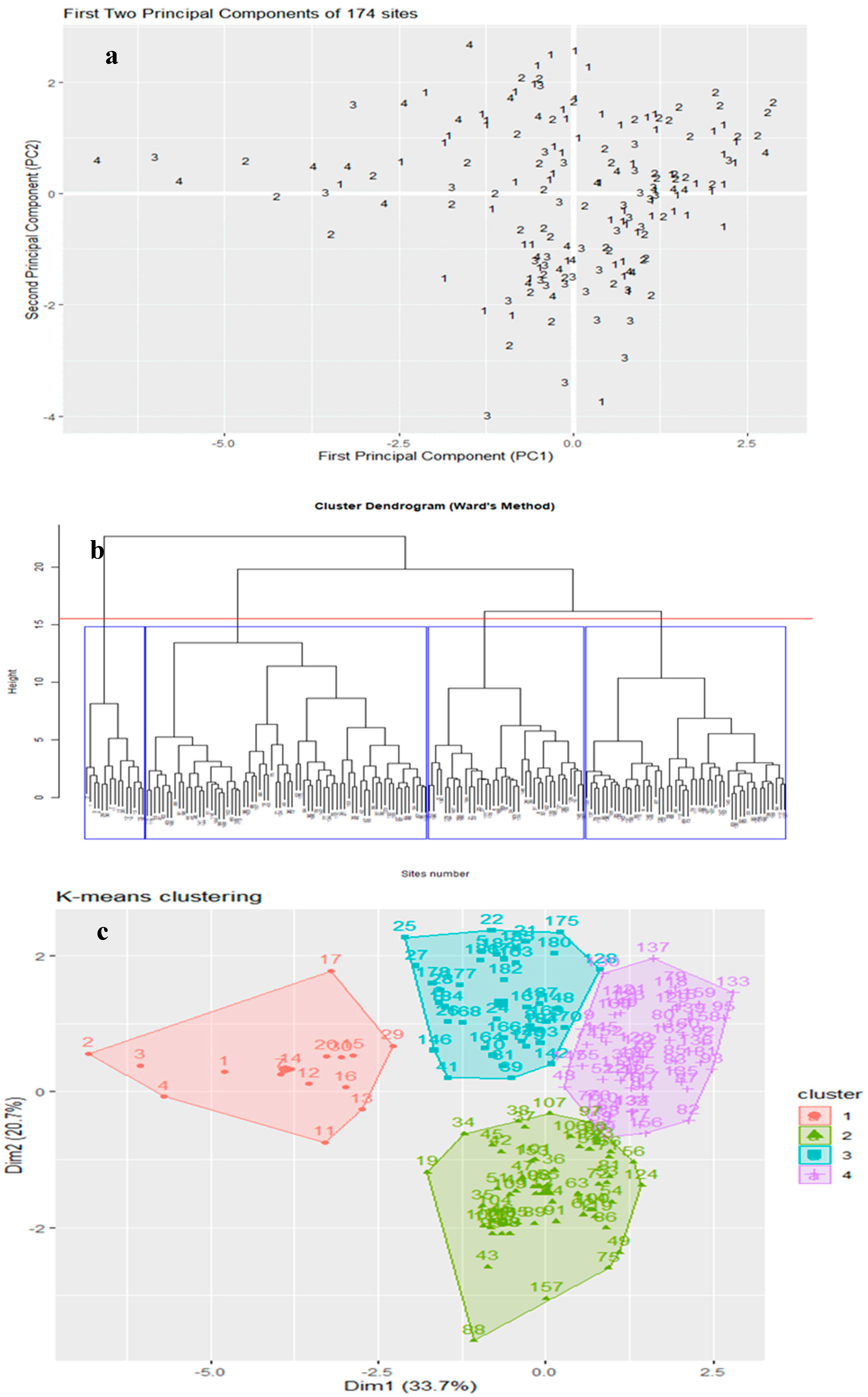
2.3.3. Multivariate Statistical Analysis

To compare groups formed in the LCV-LSK space (four largest homogeneous regions, n = 174, see Section 2.3.1), we applied principal component analysis (PCA) and cluster analysis. Through this analysis, it was examined whether there is any association between the LCV-LSK space and the catchment and climate characteristics data space.

Principal Component Analysis (PCA)

A data reduction technique, PCA transforms an original set of variables to a new set of mutually uncorrelated variables arranged in decreasing order of importance. This new set of variables are called principal components (PCs). The first PC (PC1) is the linear combination of the original variables, which captures as much of the variation in the original data set as possible. The second PC (PC2) captures the maximum variability that is uncorrelated with PC1, and so on. The PC’s number is equal to the number of original input variables in the data set.

Cluster Analysis

The main goal of cluster analysis is to form mutually exclusive and exhaustive groups of observations, which ensure similarity of observations within a group (homogeneous) and dissimilarity between groups (heterogeneous). Cluster analysis refers to a wide range of techniques where almost all methods require a measure of similarity or dissimilarity between observations. In this study we adopted (i) Ward’s method [33], a hierarchical agglomeration method, and (ii) K-means clustering, a centroid-based method. Ward’s method is the minimum-variance method and provides reasonable groupings in most cases [34,35]. In merging two clusters from the previous generation, the sum of squares is minimized over all the partitions at every stage. The most used and the simplest centroid-based clustering method is K-means clustering, which is an unsupervised machine learning algorithm [36,37]. It splits a dataset comprising of n observations into a set of k groups (k-clusters). It minimizes squared Euclidean distance (within-cluster variances) but not regular Euclidean distance. It also classifies the objects into multiple clusters in such a way that within clusters the similarity among objects is as high as possible (i.e., high intra-class similarity) and between clusters it is as dissimilar as possible (i.e., low inter-class similarity). In K-means clustering, each cluster has a mean (centroid) for its points, and it represents the cluster. In hydrology, Ward’s method and K-means clustering are commonly used because of their consistent performances [38,39,40,41].

2.3.4. Prediction Model Development

In RFFA, the at-site flood frequency analysis (FFA) is the first step where an appropriate probability distribution is fitted to the AM flood data. In this study, log-Pearson Type 3 (LP3) distribution (Bayesian fitting) was used using FLIKE software version 1.0 [42], which has been incorporated in Australian Rainfall and Runoff (ARR) [42,43,44]. Previous Australian studies found that the LP3 distribution is the most appropriate distribution for at-site FFA for the majority of Australian catchments and hence it was adopted in this study [28,45]. Flood quantiles were estimated for six return periods (T)/annual exceedance probabilities (AEPs), which were used as dependent variables in prediction model development.

Among various regional flood estimation models, the QRT is widely used for its simplicity and better performances [46,47,48]. This QRT model was proposed by the United States Geological Survey (USGS) to develop prediction equations [49]. In this study, the ordinary least square (OLS) method was used to estimate the regression coefficients. It should be noted that the PRT is the alternative to the QRT. In the PRT, parameters of a selected probability distribution (such as LP3) are regionalized [28]. In this study, we adopted the QRT as previous studies showed that both the QRT and PRT performed similarly for southeast Australia [28].

Mathematically, the QRT can be expressed as:

Q_T = aB^bC^cD^d …

(1)

where Q_T is the flood quantile for T years return period; B, C, D, … refer to the catchment characteristics (predictors), and a, b, c, … are regression coefficients estimated by the OLS method.

Applying selected predictors and taking the log (base 10) transformation, Equation (1) can be simplified as:

$$\begin{gathered} {log}_{10}\left(Q_T\right)=b_0+b_1* {log}_{10}\left(\mathit{AREA}\right)+b_2* {log}_{10}\left(I_{62}\right)+b_3* {log}_{10}\left(\mathit{MAR}\right)+b_4* \\ {log}_{10}\left(\mathit{SF}\right)+b_5* {log}_{10}\left(\mathit{MAE}\right)+b_6* {log}_{10}\left(\mathit{SDEN}\right)+b_7* {log}_{10}\left(S1085\right)+b_8* \\ {log}_{10}\left(\mathit{FOREST}\right) \end{gathered}$$

(2)

where Q_T, is the flood quantile for AEP of 1 in T.

The IFM was first proposed by Dalrymple [15]. The IFM is well explained by Hosking and Wallis (1997) [50]. It is considered one of the most efficient [51] RFFA methods [46,52,53] based on a hypothesis that floods at the various sites of a region are identically distributed except for a site-specific scaling factor, or the index flood, which is generally a function of catchment physiographic characteristics. Generally, the mean or median of AMF data is used as a scaling factor [54]. The IFM has been applied by many researchers [34,47,55,56,57,58,59,60]. Bobee et al. [46] suggested that, despite there being some critiques of the IFM, a general procedure proposed by Dalrymple [15] for the delineation of homogeneous regions remains one of the most popular approaches to RFFA.

Mosaffaie [61], described the IFM as follows: Say data are available at N sites with site i having sample size n_i and observed AMF data Q_ij (j = 1, …, n_i). Q_i (F), 0 < F < 1, is the quantile function of frequency distribution at site i. The key assumption of the IFM is that the sites form a homogeneous region, that is, the frequency distributions of the N sites are identical apart from a site-specific scaling factor, the index flood.

$$\begin{gathered} Q_{\mathrm{i}}\left(F\right)={\mu }_{\mathrm{i}}\mathrm{q}\left(F\right), i=1, \dots , N \\ \mathrm{or} Q_i^T={\mu }_i{q}_T \end{gathered}$$

(3)

where $Q_T^i$ is the flood quantile corresponding to a T-year return period at a given site i. The index flood is naturally estimated by μ_i = $\overline{Q}$_i, the sample mean of the AMF data at site i. Other location estimators such as the median or a trimmed mean could be used instead. μ_i is supposed to be the mean of the at-site frequency distribution, q(F) is the regional quantile of non-exceedance probability F, and $q_T$ is the regional quantile of the return period T [61].

2.3.5. Validation Approach and Evaluation Criteria

In RFFA, the leave-one-out (LOO) validation approach is commonly used to validate the developed prediction equations [62]. In this process, one catchment is left out to develop a prediction equation, and then this equation is tested on the left-out catchment, and the procedure is repeated with all the catchments of a given region. Adopting the LOO technique, the below seven evaluation criteria were used to evaluate the developed predictions for the assumed regions:

$$Relative error (RE)={\displaystyle \frac{Q_{pred}-Q_{obs}}{Q_{obs}}}\times 100$$

(4)

$$Absolute median relative error (AMRE)=median\left[abs\left({\displaystyle \frac{Q_{pred}-Q_{obs}}{Q_{obs}}}\right)\right]\times 100$$

(5)

$$Mean square error (MSE)=mean\left[{\left(Q_{pred}-Q_{obs}\right)}^2\right]$$

(6)

$$Bias (BIAS)=mean\left(Q_{pred}-Q_{obs}\right)$$

(7)

$$Relative Bias (RBIAS)=\left[mean\left({\displaystyle \frac{Q_{pred}-Q_{obs}}{Q_{obs}}}\right)\right]\times 100$$

(8)

$$Relative root mean square error (RRMSE)={\displaystyle \frac{\sqrt{\left[{mean\left(Q_{pred}-Q_{obs}\right)}^2\right]}}{{mean[Q}_{obs}]}}$$

(9)

$$Root mean square normalized error (RMSNE)=\sqrt{{[mean\left({\displaystyle \frac{Q_{pred}-Q_{obs}}{Q_{obs}}}\right)}^2]}$$

(10)

The at-site flood quantiles (Q_obs) were obtained by fitting the LP3 distribution to the AMF data (see Section 2.3.4) and the predicted flood quantiles (Q_pred) were estimated applying the developed prediction equations (Equation (2)). R was used to perform regression analysis and Python 3.11.4 was used to prepare spatial maps.

3. Results

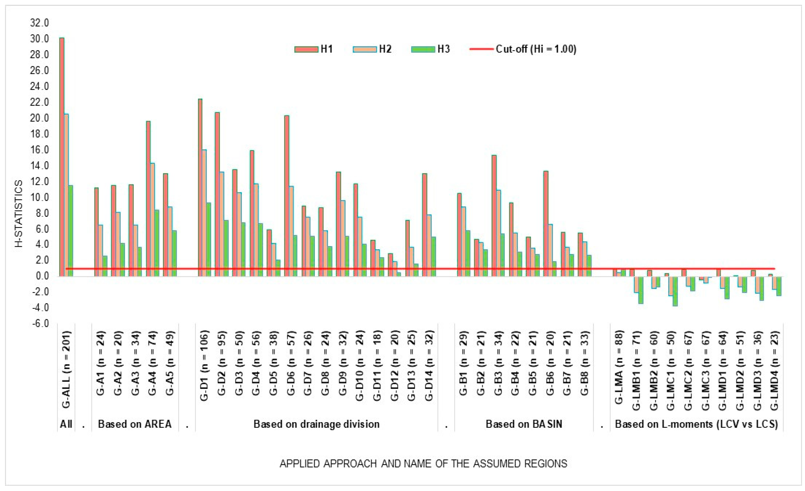
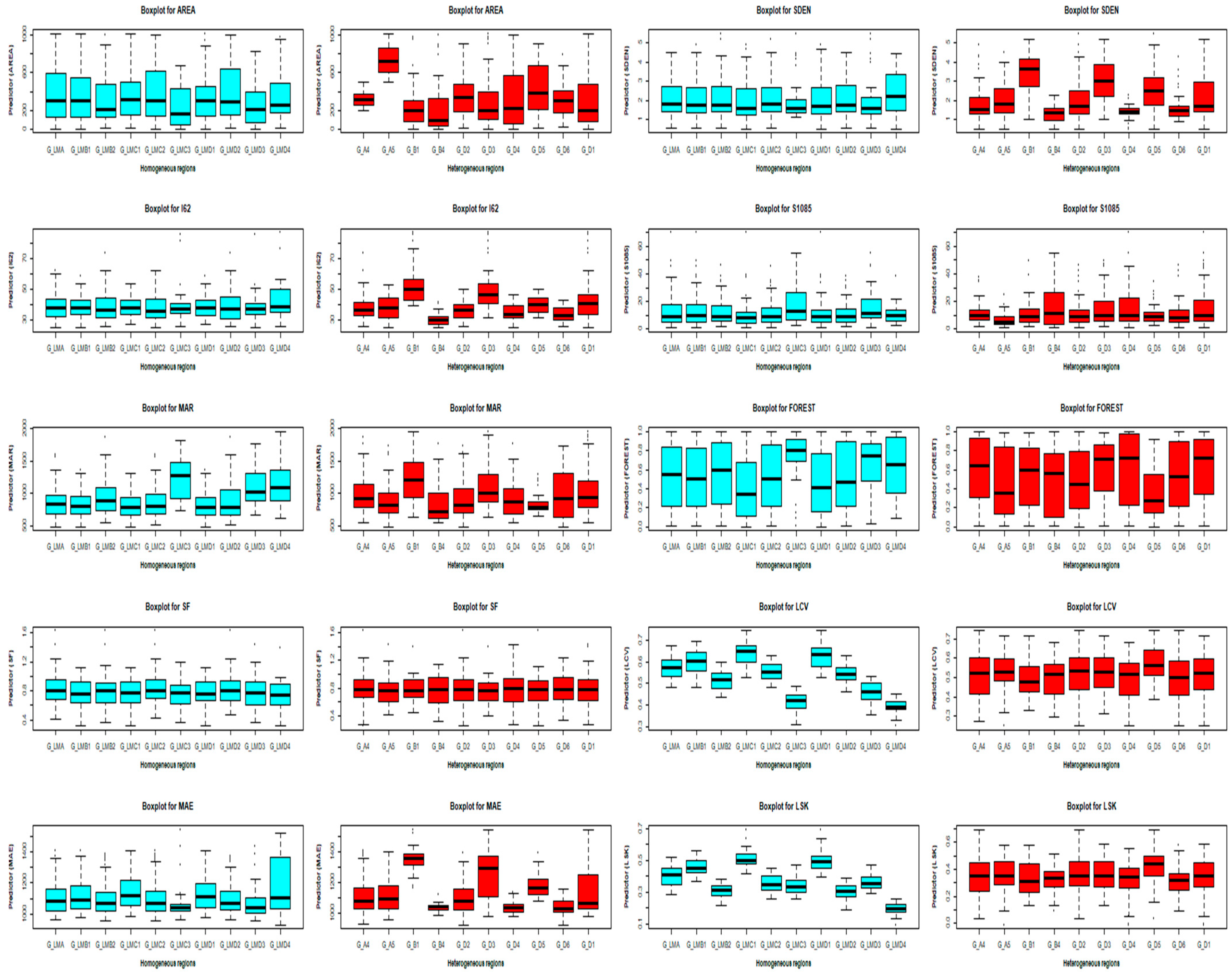
3.1. Discordancy and Homogeneity Assessment of the Formed Regions

Table 1 presents summary results of all the assumed regions based on different approaches (see Section 2.3.1). It refers to the notation of regions, number of sites in each region, the lowest and the highest D_i values (only for the discordant sites), and H- and Z-statistics. Hosking and Wallis [16] assessment criteria for testing discordancy and homogeneity were used here. Placing 201 sites in a single region (G-ALL), 9 sites were detected as discordant for the region. In this case, the discordant values range from 3.26 to 6.43. In regions G-D2, G-D6, and G-D14, the D_i statistic ranges from 3.05 to 7.18, 3.16 to 5.80, and 3.11 to 6.45, respectively. The removal of discordant sites from these regions does not reduce Di values significantly; hence, this study considered all the selected sites for further analysis. No discordant site was found in regions G-D7, G-D12, G-D13, G-B1, G-B4, G-B5, G-B7, and G-LMD2.

Except the regions formed based on the LCV-LSK space, all other regions are highly heterogenous (H₁-statistics >> 1). The highest H₁-value (30.13) was found in the region G-ALL followed by G-D1 (H₁ = 22.41), G-D2 (H₁ = 20.78), and G-D6 (H₁ = 20.34). Among the heterogeneous regions, the lowest H₁-value was found in the region G-D12 (H₁ = 2.86) followed by G-D11 (H₁ = 4.57). Among the heterogeneous regions, the region G-D12 selected all the distributions as acceptable with Z-values < 1.64; in contrast, there was no acceptable distribution for regions G-LMB2, G-LMC3, and G-LMD2 as Z-values > 1.64. With some exceptions, Pearson Type 3 (PE3) and Generalized Pareto (GPA) were found to be the best-fit distributions for the majority of the proposed regions.

Figure 4 compares the H_i-statistics among all the assumed regions. It clearly shows that all the regions are highly/definitely heterogeneous (far away from the threshold value of 1.00, indicated by the red line) except the regions formed based on the LCV-LSK space. The region G-A4 (n = 74) has the highest H₁ value (19.62) compared to other regions. Among contiguous basin-based regions, the highest H₁ statistic is 15.34. Figure 3 also shows that the H_i -statistics are higher in the regions based on drainage division, followed by AREA and basin. A general statement can be made from this figure: “the more the number of sites in a region the higher the H_i values are, and H₁ > H₂ > H₃”.

3.2. Prediction Model Evaluation

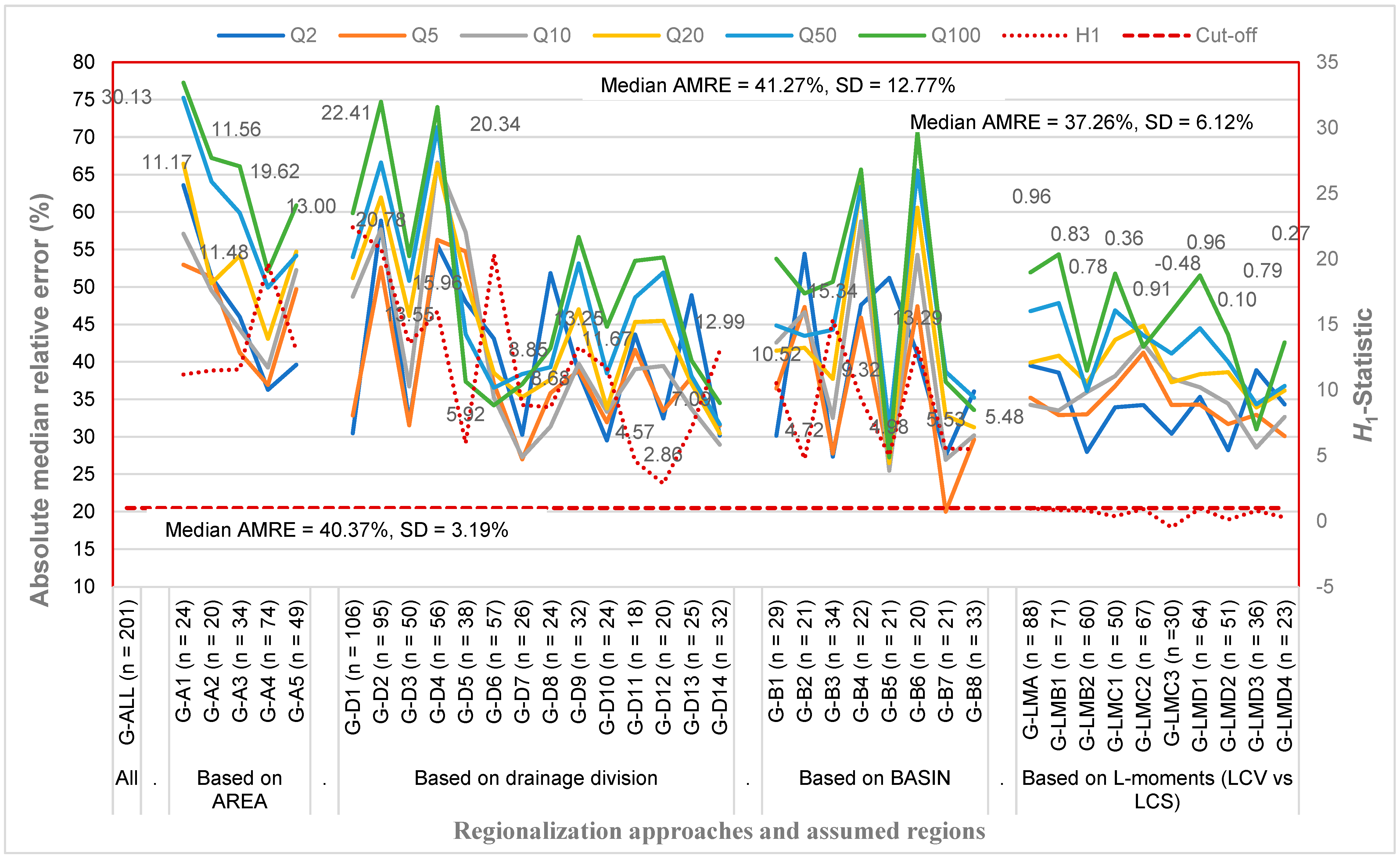
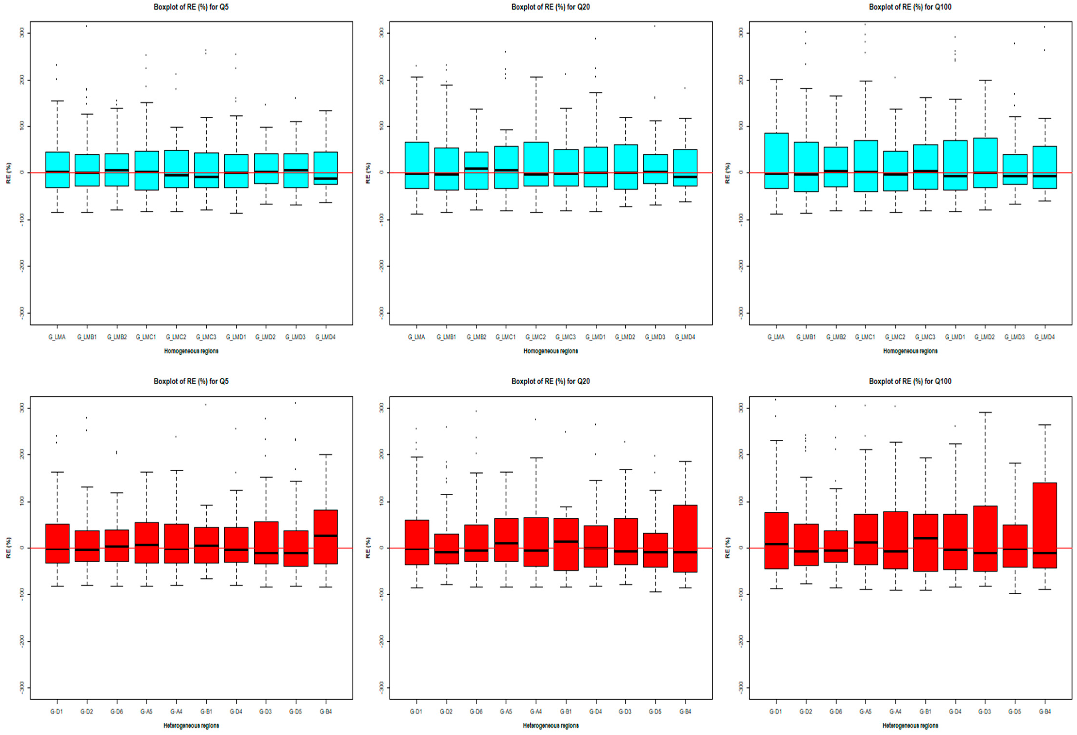
3.2.1. Degree of Heterogeneity vs. Absolute Median Relative Error

Figure 5 compares the H_i values and absolute median relative error (AMRE) estimated from the developed QRT for each of the assumed regions. It also examines the association between the degree of heterogeneity and AMRE (%).

With the highest H₁-value (30.13), the single region (G-ALL, n = 201) shows relatively lower AMRE values (below 46%). These values range from 36.98 (Q₁₀) to 45.34 (Q₁₀₀). In contrast, the region G-A1 (n = 24) exhibits the highest AMRE values (77.27% for Q₁₀₀) with a moderate H₁-value (11.17). Similarly, the regions G-D2 (n = 95), G-D4 (n = 56), G-B4 (n = 22), and G-B6 (n = 20) also show higher AMRE values. For Q₁₀₀, these values are 74.70%, 73.99%, 65.66%, and 70.62% having the H₁-statistics 20.78, 15.96, 9.32, and 13.29, respectively. The lowest 20.01% (Q₅) and the second lowest 25.48% (Q₁₀) AMRE values are found in the region G-B7 (n = 21, H₁-value 5.53) and region G-B5 (n = 21, H₁-value 4.98), respectively. Moreover, a significant number of AMRE values of quantile estimates are found below 30.00% in some regions with H₁-value ranging from 0.10 to 15.34. These are: 26.98% (Q₅) and 27.29% (Q₁₀) in region G-D7, 29.50% (Q₂) in region G-D10, 28.93% (Q₁₀) in region G-D14, 27.35% (Q₂) and 27.75% (Q₅) in region G-B3, 26.76% (Q₅), 26.51% (Q₂₀), and 27.26% (Q₁₀₀) in region G-B5, 27.49% (Q₂) and 26.93% (Q₁₀) in region G-B7, 27.98% (Q₂) in region G-LMB2, 28.21% (Q₂) in region G-LMD2, and 28.55% (Q₁₀) in region G-LMD3.

The AMRE value of flood quantile estimates is roughly below 40.00% for the regions G-D6 (except Q₂), G-D7, G-D10 (except Q₁₀₀), G-D13 (except Q₂), G-B7, G-B8, G-LMB2, and G-LMD4 (except Q₁₀₀). Noteworthy, it is below 35.00% for the regions G-D14, G-B5 (except Q₂), and G-LMD3 (except Q₂). Over the quantiles, the median AMRE value for the fixed single region is 40.37% with a standard deviation (SD) of 3.19%. Among the regions under a categorical approach, say AREA, drainage division, basin, and L-moments space, the median values are 52.17% (SD = 10.68%), 39.61% (SD = 11.61%), 41.27% (SD = 12.77%), and 37.26% (SD = 6.12%), respectively. The overall median AMRE value of the quantile estimates among all the assumed regions is 40.09% (SD = 11.35%).

In RFFA, generally it is believed that the more the regional homogeneity is, the more accurate the flood quantiles estimate is. The assumed regions based on a single fixed region, AREA, drainage division, and basin are highly heterogeneous (H₁-values range from 2.86 to 30.13), and regions based on the LCV-LSK space are acceptably homogeneous (H₁-values range from −0.48 to 0.96). In these homogeneous regions, the AMRE values are lower compared to other regions, which range from roughly 28% to 55%. Irrespective of this homogeneity (heterogeneity) condition, the AMRE values do not decline (increase) over the quantiles, which does not support the usual notion of RFFA. Hence, little association was found between the degree of heterogeneity and the accuracy of the model estimates (AMRE) in southeast Australia.

3.2.2. Model Evaluation Adopting Evaluation Statistics

Table 2. Summary of evaluation statistics for the assumed regions (Q₂ to Q₁₀₀, QRT).

Evaluation Criteria	QT	All	Based on AREA					Based on BASIN								Based on L-Moments (LCV vs. LSK)
		G-ALL	G-A1	G-A2	G-A3	G-A4	G-A5	G-B1	G-B2	G-B3	G-B4	G-B5	G-B6	G-B7	G-B8	G-LMA	G-LMB1	G-LMB2	G-LMC1	G-LMC2	G-LMC3	G-LMD1	G-LMD2	G-LMD3	G-LMD4
AMRE	Q2	39.49	63.57	51.29	46.00	36.27	39.61	30.46	58.84	31.96	55.55	48.02	43.09	30.27	51.84	39.49	38.55	27.98	33.92	34.23	30.41	35.31	28.21	38.87	34.32
	Q5	37.80	52.96	51.29	41.25	36.93	49.70	32.84	52.59	31.52	56.28	54.72	37.11	26.98	35.82	35.22	32.90	32.99	36.76	41.22	34.23	34.30	31.68	32.94	30.09
	Q10	36.98	57.09	49.51	44.29	39.22	52.24	48.69	57.69	36.73	66.61	57.30	35.26	27.29	31.34	34.25	33.50	35.95	38.10	42.40	37.78	36.59	34.41	28.55	32.65
	Q20	41.24	66.45	50.50	54.16	43.08	54.71	51.19	61.94	46.11	66.38	51.06	38.52	35.29	37.63	39.89	40.81	37.23	42.94	44.82	37.28	38.36	38.62	33.91	36.18
	Q50	43.04	75.25	64.06	59.89	49.92	54.17	53.97	66.60	50.81	71.31	43.69	36.54	38.38	39.29	46.77	47.85	36.11	46.86	43.53	41.11	44.49	39.99	34.34	36.78
	Q100	45.34	77.27	67.21	66.10	52.09	60.87	59.84	74.70	54.12	73.99	37.37	34.19	37.02	41.81	51.93	54.34	38.81	51.77	42.01	46.73	51.53	43.60	30.99	42.59
MSE	Q2	2514.73	401.48	1465.38	1823.47	2877	6770	5380	11,839	1493	314	7621	1648	206	1717	1712	820	2326	736	2902	1736	696	2365	3095	3592
	Q5	13,166.85	4380.66	5373.60	19,734.92	141,92	36,263	25,387	121,274	7202	3125	56852	12,797	1223	8141	15,615	8780	13,864	7781	18,165	11,708	6840	13,760	17,213	10,520
	Q10	36,474.56	39,183.65	14,464.86	87,771.38	35,444	103,510	73,838	485,875	18,771	10,417	78,074	31,879	2836	27,302	51,647	33,843	38,813	29,589	47,928	33,542	25,244	46,210	40,808	18,951
	Q20	94,459.31	222,126.95	38,891.46	306,740.34	801,88	278,231	204313	1,856,370	44,676	26,355	80,394	58,223	6080	89,060	147,390	108,650	98,994	96,021	108,083	88,894	80,540	143,457	81,729	31,368
	Q50	309,516.46	1,429,884.04	132,519.97	1,247,388.99	216,832	952,076	726,152	11,728,100	128,854	69,605	86,694	99,656	16,226	377,765	511,950	426,355	308,162	392,278	271,005	297,021	327,252	546,552	175,799	56,678
	Q100	722,328.06	4,760,233.15	309,416.08	3,155,874.16	440,854	2,273,787	1,787,504	50,031,260	274,128	128,601	106,835	134,021	33,252	1,026,171	1,210,574	1,091,092	676,944	1,044,854	501,192	691,407	875,336	1,340,578	291,266	85,604
RMSE	Q2	50.15	20.04	38.28	42.70	53.64	82.28	73.35	108.81	38.64	17.73	87.30	40.60	14.36	41.44	41.38	28.63	48.23	27.12	53.87	41.67	26.38	48.63	55.64	59.94
	Q5	114.75	66.19	73.30	140.48	119.13	190.43	159.33	348.24	84.86	55.90	238.44	113.12	34.98	90.23	124.96	93.70	117.74	88.21	134.78	108.20	82.71	117.30	131.20	102.57
	Q10	190.98	197.95	120.27	296.26	188.27	321.73	271.73	697.05	137.01	102.06	279.42	178.55	53.26	165.23	227.26	183.97	197.01	172.01	218.93	183.14	158.88	214.97	202.01	137.66
	Q20	307.34	471.30	197.21	553.84	283.17	527.48	452.01	1362.49	211.37	162.34	283.54	241.29	77.98	298.43	383.91	329.62	314.63	309.87	328.76	298.15	283.80	378.76	285.88	177.11
	Q50	556.34	1195.78	364.03	1116.87	465.65	975.74	852.15	3424.63	358.96	263.83	294.44	315.68	127.38	614.63	715.51	652.96	555.12	626.32	520.58	545.00	572.06	739.29	419.28	238.07
	Q100	849.90	2181.80	556.25	1776.48	663.97	1507.91	1336.98	7073.28	523.57	358.61	326.86	366.09	182.35	1013.00	1100.26	1044.55	822.77	1022.18	707.95	831.51	935.59	1157.83	539.69	292.58
BIAS	Q2	−9.53	1.95	−4.49	−3.11	−10.69	−14.87	−1.19	−4.77	−4.00	0.69	13.60	6.91	−0.51	−3.90	−6.60	−3.33	−9.12	−3.37	4.67	−5.71	−3.17	−7.32	−3.60	2.58
	Q5	−20.05	11.93	−6.62	1.92	−22.53	−33.48	−3.93	6.31	−9.05	5.14	38.47	17.62	−1.60	−4.06	−20.98	−10.89	−20.82	−9.72	15.63	−16.75	−10.10	−17.69	−6.26	1.24
	Q10	−33.25	35.29	−9.07	12.21	−35.30	−54.46	−8.99	46.25	−16.06	10.98	37.54	27.87	−2.72	−5.98	−39.96	−22.48	−32.62	−18.65	27.79	−31.10	−20.13	−30.58	−8.42	−0.71
	Q20	−54.95	84.52	−14.31	29.21	−53.97	−86.77	−18.68	157.56	−27.56	18.27	23.64	38.88	−4.17	−12.96	−70.42	−42.92	−48.03	−34.68	44.17	−53.78	−37.49	−50.94	−10.85	−3.56
	Q50	−105.44	217.69	−29.53	63.48	−93.06	−158.96	−43.39	579.62	−53.76	28.89	−3.76	53.31	−6.65	−37.93	−138.35	−93.15	−76.03	−75.99	73.34	−103.19	−79.87	−95.21	−14.91	−8.77
	Q100	−169.16	401.23	−51.45	98.56	−138.97	−248.34	−76.41	1375.82	−86.32	36.63	−26.68	63.62	−8.85	−77.51	−220.83	−159.53	−104.73	−133.30	102.11	−161.54	−135.94	−147.16	−19.10	−13.95
RBIAS	Q2	22.24	396.41	40.60	26.60	21.75	20.11	15.81	61.28	11.83	36.06	83.04	48.34	8.72	36.78	18.83	19.18	13.13	28.15	41.89	16.32	25.32	10.09	19.12	26.48
	Q5	21.41	143.52	25.59	22.07	21.57	21.49	14.02	88.51	16.88	36.50	126.99	58.18	14.34	21.88	20.34	20.19	12.38	29.65	47.21	14.25	28.67	8.89	18.86	23.20
	Q10	23.55	103.03	26.32	26.38	24.60	24.51	18.68	114.99	21.74	43.45	110.31	64.74	16.90	20.94	21.81	22.78	12.67	30.26	50.66	13.85	30.34	9.72	18.05	22.70
	Q20	26.91	96.27	30.90	33.26	28.92	28.45	25.54	150.41	27.05	51.65	82.72	69.92	19.31	23.15	23.80	26.07	13.31	31.41	54.27	14.10	31.98	11.22	17.00	23.03
	Q50	32.76	110.88	41.81	45.26	36.11	34.94	37.05	215.27	34.74	63.48	52.10	75.67	22.76	28.87	27.31	31.45	14.77	34.27	59.14	15.44	34.69	14.15	15.62	24.44
	Q100	38.13	133.48	53.75	56.29	42.51	40.80	47.40	282.46	41.11	73.15	37.18	79.77	25.73	34.66	30.66	36.34	16.35	37.60	63.04	17.22	37.44	17.03	14.73	26.11
RRMSE	Q2	0.15	0.15	0.10	0.07	0.16	0.14	0.01	0.05	0.08	0.03	0.28	0.16	0.02	0.06	0.11	0.07	0.11	0.08	0.10	0.08	0.08	0.08	0.07	0.02
	Q5	0.13	0.39	0.06	0.02	0.14	0.13	0.01	0.02	0.08	0.10	0.37	0.20	0.02	0.02	0.12	0.08	0.11	0.07	0.17	0.09	0.07	0.08	0.06	0.01
	Q10	0.13	0.71	0.05	0.07	0.14	0.13	0.02	0.09	0.09	0.14	0.25	0.23	0.02	0.02	0.13	0.09	0.11	0.07	0.22	0.10	0.08	0.09	0.05	0.00
	Q20	0.15	1.15	0.06	0.11	0.15	0.13	0.03	0.21	0.10	0.16	0.12	0.25	0.02	0.03	0.15	0.10	0.12	0.08	0.26	0.12	0.09	0.10	0.05	0.01
	Q50	0.18	1.87	0.07	0.16	0.17	0.15	0.04	0.45	0.13	0.18	0.01	0.27	0.03	0.04	0.18	0.13	0.13	0.09	0.31	0.15	0.10	0.12	0.05	0.02
	Q100	0.21	2.52	0.09	0.18	0.19	0.17	0.05	0.76	0.16	0.18	0.08	0.27	0.03	0.06	0.20	0.15	0.14	0.11	0.35	0.17	0.12	0.14	0.05	0.02
RMSNE	Q2	0.93	17.97	1.52	1.00	0.86	0.80	0.75	1.99	0.57	0.97	3.11	1.53	0.52	1.08	0.83	0.76	0.59	1.04	1.55	0.75	0.95	0.55	0.84	1.05
	Q5	0.95	5.47	0.99	0.81	0.88	0.93	0.70	2.74	0.72	1.09	5.15	1.93	0.76	0.82	0.86	0.81	0.54	1.15	1.73	0.65	1.14	0.48	0.82	0.94
	Q10	1.03	3.19	1.00	0.93	1.01	1.03	0.80	3.50	0.83	1.27	4.44	2.10	0.88	0.84	0.90	0.90	0.55	1.11	1.86	0.61	1.17	0.50	0.80	0.91
	Q20	1.13	2.60	1.13	1.13	1.18	1.14	0.95	4.49	0.93	1.46	3.23	2.22	0.97	0.95	0.95	1.00	0.56	1.08	2.01	0.60	1.18	0.53	0.77	0.91
	Q50	1.29	3.05	1.44	1.48	1.44	1.30	1.22	6.35	1.07	1.72	1.89	2.35	1.07	1.15	1.05	1.18	0.59	1.10	2.21	0.61	1.18	0.60	0.74	0.94
	Q100	1.42	3.90	1.78	1.80	1.66	1.43	1.49	8.38	1.17	1.93	1.29	2.44	1.14	1.34	1.14	1.33	0.63	1.16	2.37	0.64	1.20	0.67	0.72	0.98
R2	Q2	0.72	0.73	0.81	0.71	0.51	0.59	0.93	0.55	0.86	0.79	0.82	0.75	0.93	0.73	0.70	0.70	0.82	0.75	0.80	0.81	0.74	0.89	0.85	0.92
	Q5	0.73	0.72	0.86	0.69	0.53	0.57	0.93	0.52	0.83	0.80	0.85	0.67	0.88	0.84	0.69	0.69	0.83	0.72	0.78	0.82	0.71	0.88	0.85	0.93
	Q10	0.72	0.69	0.87	0.67	0.54	0.57	0.90	0.50	0.79	0.78	0.87	0.63	0.85	0.87	0.69	0.67	0.83	0.71	0.78	0.82	0.69	0.88	0.86	0.93
	Q20	0.70	0.66	0.87	0.66	0.54	0.58	0.87	0.48	0.75	0.75	0.88	0.60	0.81	0.87	0.69	0.66	0.83	0.69	0.77	0.82	0.68	0.87	0.86	0.93
	Q50	0.68	0.62	0.86	0.64	0.54	0.57	0.81	0.46	0.70	0.72	0.89	0.57	0.78	0.85	0.69	0.64	0.82	0.67	0.76	0.81	0.66	0.86	0.87	0.93
	Q0	0.66	0.59	0.84	0.63	0.53	0.57	0.76	0.45	0.67	0.70	0.89	0.54	0.76	0.84	0.68	0.63	0.81	0.65	0.76	0.80	0.65	0.84	0.88	0.93

shows the value of evaluation criteria estimated from the developed prediction equations using the QRT. The highest and the lowest AMRE values among all the assumed regions are 20.01% (Q₅) in G-A1 and 77.27% (Q₁₀₀) in G-D13, respectively. The estimated MSE values lie in a range of 206.09 (Q₅) in G-B7 to 50031260.38 (Q₁₀₀) in G-B2. Interestingly, these figures for RMSE values range from 14.36 (Q₅ in G-B7) to 7073.28 (Q₁₀₀ in G-B2). The maximum BIAS and RBIAS values for the developed models are 1375.82 (Q₁₀₀ in G-B2) and 396.41 (Q₂ in G-A1), respectively. The minimum values for these are −248.34 (Q₁₀₀ in G-A5) and 8.72 (Q₂ in G-B7), respectively. The lowest value of RRMSE (0.00) is found in region G-LMD4 (Q₁₀) and G-D11 (both Q₅ and Q₅₀,) and the highest (2.52) one is in G-A1 for Q₁₀₀. The RMSNE value varies for the developed models from 0.48 (Q₅) in region G-LMD2 to 17.97 (Q₂) in region G-A1. The value of regression coefficient of determination (R²), which quantifies the strength of the model, fluctuates from 0.45 (Q₁₀₀ in G-B2) to 0.94 (Q₁₀ in G-D11).

Figure 6 compares the RE (%) value estimated for flood quantiles Q₅, Q₂₀, and Q₁₀₀ from the developed prediction equations adopting QRT (Figure S5 illustrates RE values for all the six quantiles). The first row in Figure 5 represents ten homogeneous regions based on LCV-LSK space and the second row refers to ten heterogeneous regions. The parallel sequential region consists of a nearly similar number of sites. Here the “0” line refers to an unbiased estimate (the best-fit) between the observed and predicted values. In the region G-LMD4 vs. G-B4, the RE (%) values for Q₅ deviates from the best-fit line remarkably with a higher deviation in the heterogeneous region. Though there are some fluctuations in RE values of Q₂₀ both in homogeneous and heterogeneous regions (G-LMB2, G-LMD4, G-D2, G-A5, G-B1, and G-B4), the maximum REs of homogeneous regions touch the best-fit line. Similarly, in the case of Q₁₀₀ the RE values are skewedly distributed from the median value, say in regions G-A4, G-D3, and G-B4.

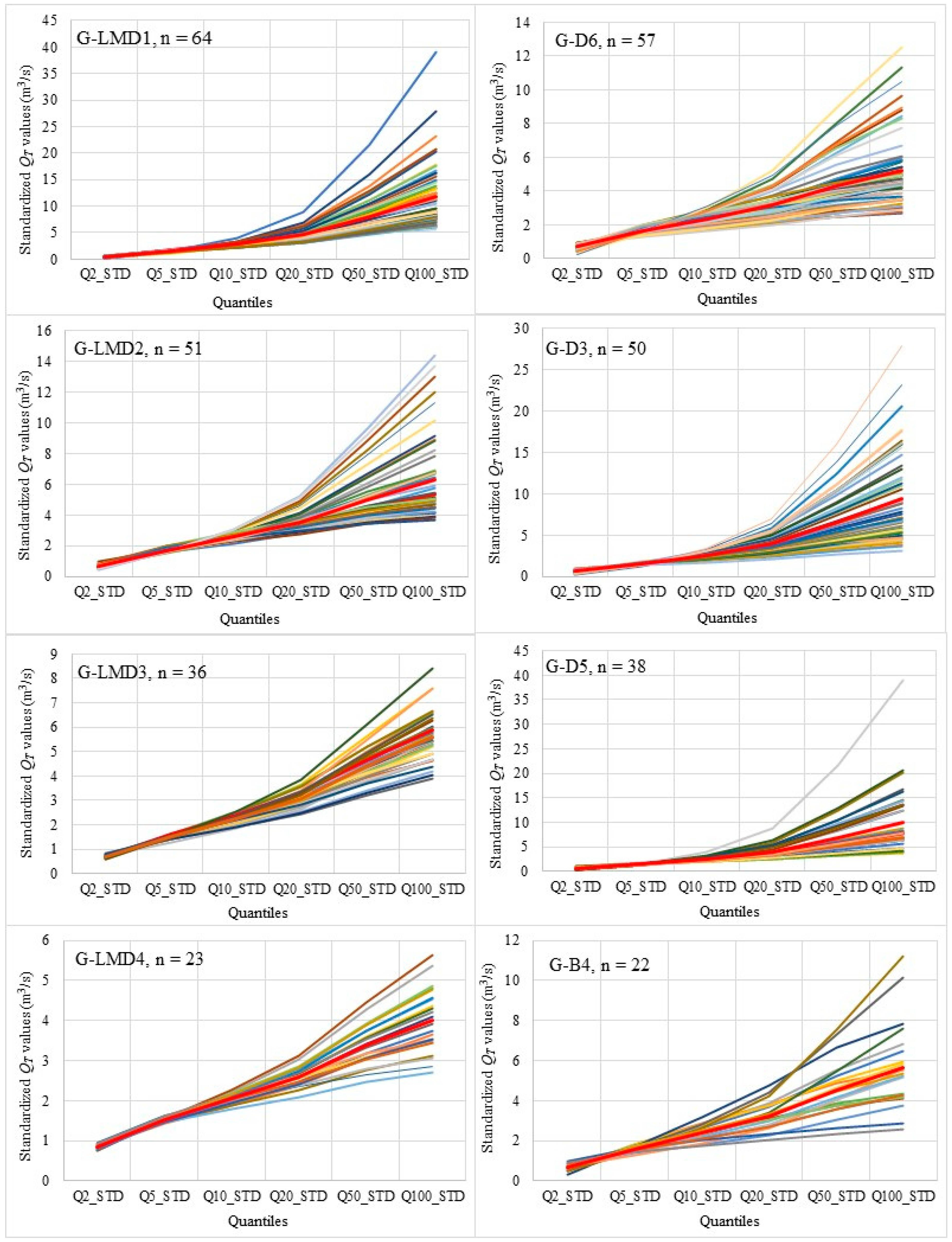
3.2.3. Comparison of Standardized Flood Frequency Curves Between the Homogeneous and Heterogeneous Regions

Figure 7 illustrates the comparison of standardized flood frequency curves (SFFCs) between homogeneous and heterogeneous regions. The four regions in the first column are the homogeneous regions formed based on the LCV-LSK space and parallelly shown (consists of nearly similar number of sites) in the second column are the regions which are heterogenous (formed based on drainage division and basin contiguity). The wider red color line shows the mean standardized value of flood quantile in each graph. The SFFCs between homogeneous and heterogeneous region (G-LMD1 vs. G-D6) are more likely to be similar for lower flood quantiles (Q₂ to Q₂₀). In the upper quantiles (Q₅₀ to Q₁₀₀), the variation is more prominent. The parallel regions G-LMD2 vs. G-D3, G-LMD3 vs. G-D5, and G-LMD4 vs. G-B4 show a similar pattern, but in the regions G-LMD3 and G-LMD4, the flood quantile estimates are more consistent. It can be said that SFFCs do not vary significantly in terms of homogeneous (or heterogeneous) conditions. In Figure 6, SFFCs for higher return periods (e.g., 100 years) show wider variation among the stations within a region for both the homogeneous and heterogeneous regions. This indicates that a higher degree of uncertainty is associated with the flood quantile estimates for the higher return periods. This is also evident in Figure 5, where the box width of the REs is larger for a 100-year return period compared to smaller return periods.

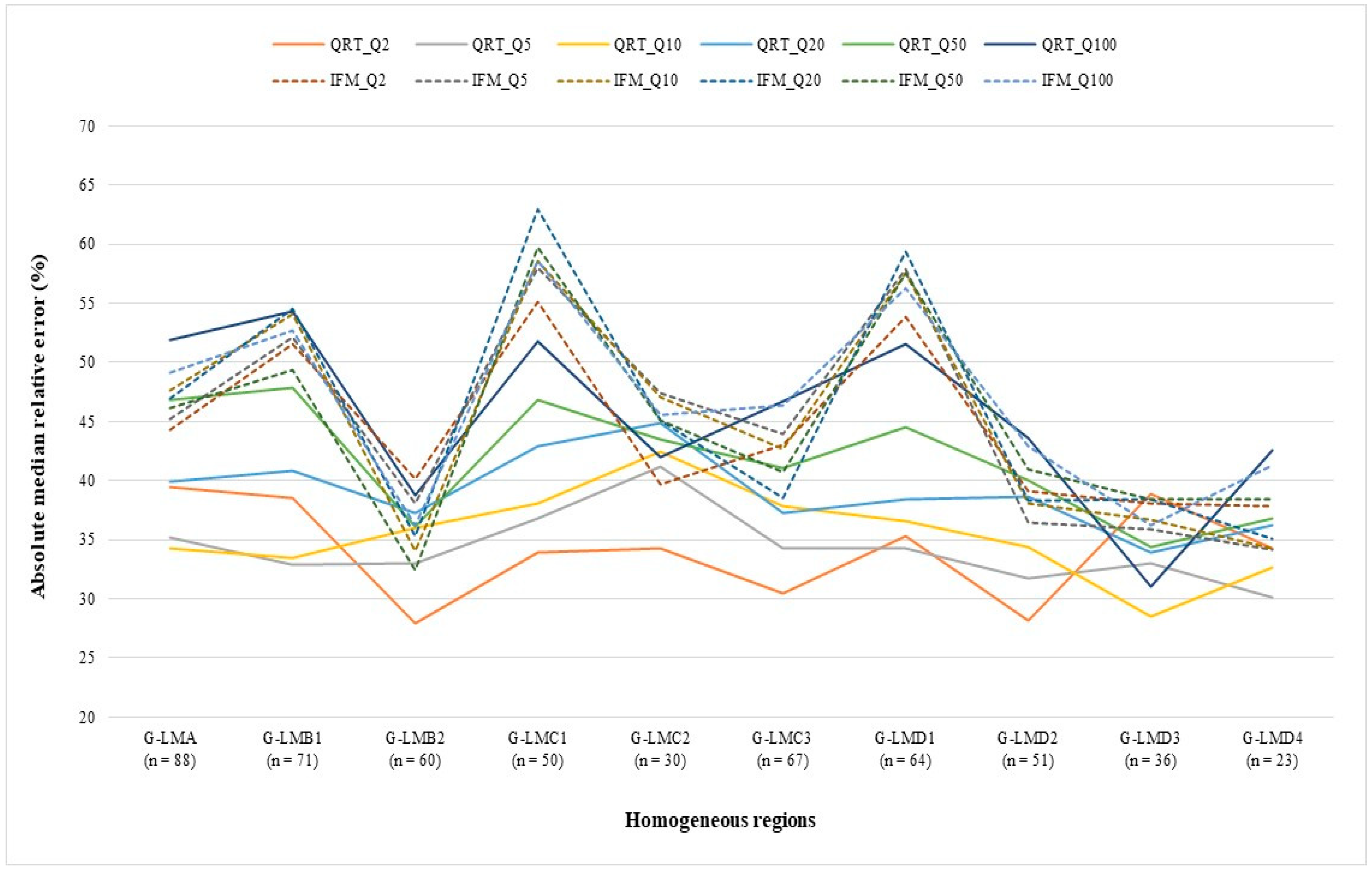
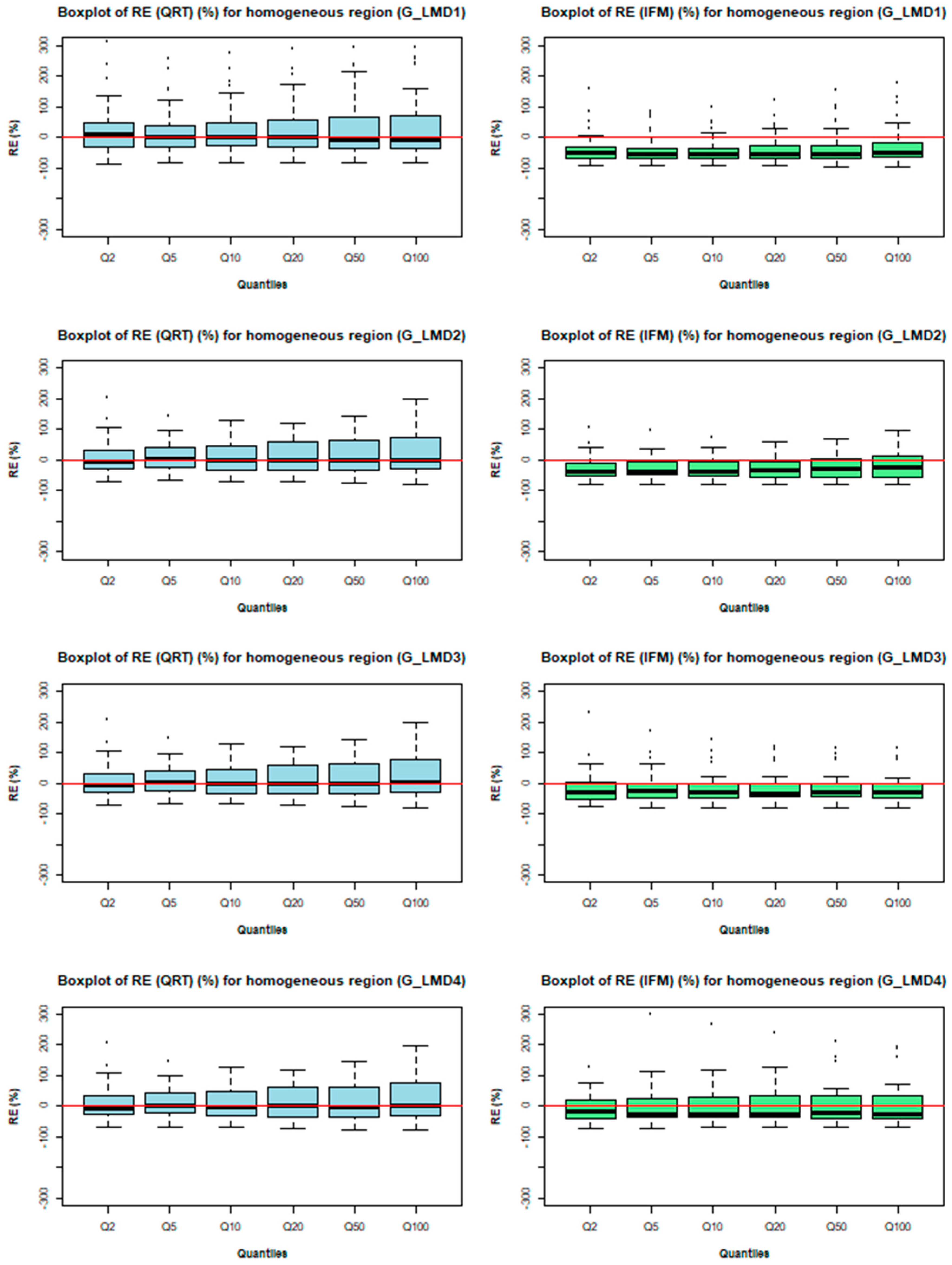
3.3. Comparison of Quantile Regression Technique (QRT) and Index Flood Method (IFM)

In this study, the IFM is used for 10 homogeneous regions (based on the LCV-LSK space) to compare the quantile estimates in terms of AMRE and the selected evaluation statistics.

Table 3. Summary of evaluation statistics for the assumed regions (Q₂ to Q₁₀₀, IFM).

Evaluation Criteria	QT	Based on L-Moments (LCV vs. LSK)
		G-LMA	G-LMB1	G-LMB2	G-LMC1	G-LMC2	G-LMC3	G-LMD1	G-LMD2	G-LMD3	G-LMD4
AMRE	Q2	44.34	51.55	40.09	55.11	39.70	43.04	53.87	39.12	38.07	37.81
	Q5	45.16	52.16	38.08	58.02	47.36	43.98	57.91	36.42	35.88	34.14
	Q10	47.61	54.07	34.08	58.57	47.01	42.62	57.50	38.07	36.74	34.21
	Q20	46.94	54.50	35.30	62.98	45.05	38.53	59.35	38.27	38.38	35.07
	Q50	46.15	49.34	32.45	59.78	45.14	40.76	57.52	41.00	38.44	38.42
	Q100	49.08	52.68	36.22	58.53	45.60	46.40	56.26	42.90	36.17	41.25
MSE	Q2	2856	1352	4017	1457	1923	3055	1326	4408	2766	3866
	Q5	25535	14,548	22,134	15,881	6937	22,212	14,187	25,240	13,691	14,161
	Q10	84,987	53,586	58,871	58,805	13,523	68,967	52,290	78,829	31,159	29,867
	Q20	238,889	162,588	138,274	180,426	23,432	186,568	159,991	219,196	61,011	57,210
	Q50	796,207	589,607	378,756	670,029	43,527	599,810	591,596	725,082	129,700	122,138
	Q100	1,811,742	1,424,691	757,186	1,656,379	65,925	1,327,169	1,455,826	1,623,676	215,182	204,411
RMSE	Q2	53.44	36.77	63.38	38.17	43.85	55.27	36.42	66.39	52.60	62.18
	Q5	159.80	120.61	148.77	126.02	83.29	149.04	119.11	158.87	117.01	119.00
	Q10	291.52	231.49	242.63	242.50	116.29	262.62	228.67	280.77	176.52	172.82
	Q20	488.76	403.22	371.85	424.77	153.07	431.93	399.99	468.18	247.00	239.19
	Q50	892.30	767.86	615.43	818.55	208.63	774.47	769.15	851.52	360.14	349.48
	Q100	1346.01	1193.60	870.16	1287.00	256.76	1152.03	1206.58	1274.24	463.88	452.12
BIAS	Q2	−29.58	−24.15	−31.14	−25.54	−7.95	−29.66	−24.32	−34.24	−17.32	−16.46
	Q5	−89.83	−77.62	−74.30	−86.00	−14.76	−80.45	−80.18	−85.58	−39.54	−34.90
	Q10	−160.31	−143.76	−118.40	−163.06	−20.41	−136.24	−150.26	−144.48	−60.40	−54.61
	Q20	−259.15	−240.23	−174.50	−277.86	−26.71	−211.12	−253.56	−225.31	−85.37	−79.81
	Q50	−447.24	−430.99	−270.92	−509.77	−36.15	−347.52	−460.10	−374.67	−125.64	−122.18
	Q100	−646.25	−639.47	−364.04	−767.95	−44.17	−486.44	−688.11	−527.84	−162.38	−161.59
RBIAS	Q2	−33.05	−40.22	−21.91	−45.23	6.97	−28.03	−43.58	−26.47	−16.55	6.58
	Q5	−33.50	−40.80	−22.60	−47.28	7.09	−29.74	−45.07	−27.91	−17.38	4.35
	Q10	−32.83	−39.31	−22.39	−46.49	7.80	−29.90	−44.11	−27.44	−17.67	3.98
	Q20	−30.99	−37.05	−21.59	−44.77	8.87	−28.90	−42.21	−25.81	−17.89	4.37
	Q50	−26.55	−32.78	−19.32	−41.16	10.60	−25.59	−38.22	−21.65	−17.97	5.93
	Q100	−21.53	−28.41	−16.58	−37.33	12.20	−21.46	−33.91	−16.85	−17.80	7.87
RRMSE	Q2	0.50	0.54	0.39	0.61	0.17	0.43	0.58	0.39	0.35	0.14
	Q5	0.52	0.55	0.39	0.60	0.16	0.44	0.58	0.38	0.36	0.16
	Q10	0.54	0.56	0.40	0.60	0.16	0.46	0.59	0.41	0.37	0.18
	Q20	0.55	0.57	0.42	0.61	0.16	0.48	0.59	0.44	0.38	0.20
	Q50	0.58	0.59	0.45	0.61	0.15	0.50	0.60	0.48	0.38	0.23
	Q100	0.59	0.60	0.47	0.61	0.15	0.52	0.60	0.51	0.39	0.25
RMSNE	Q2	0.57	0.55	0.45	0.62	1.13	0.53	0.60	0.45	0.60	0.86
	Q5	0.55	0.56	0.43	0.60	1.13	0.49	0.59	0.43	0.55	0.77
	Q10	0.55	0.57	0.43	0.60	1.15	0.48	0.59	0.43	0.53	0.73
	Q20	0.55	0.59	0.43	0.60	1.20	0.47	0.60	0.44	0.52	0.72
	Q50	0.56	0.61	0.44	0.61	1.27	0.48	0.61	0.46	0.50	0.73
	Q100	0.59	0.63	0.47	0.62	1.33	0.50	0.64	0.49	0.50	0.76
R2	Q2	0.70	0.70	0.82	0.75	0.80	0.81	0.74	0.89	0.85	0.92
	Q5	0.69	0.69	0.83	0.72	0.78	0.82	0.71	0.88	0.85	0.93
	Q10	0.69	0.67	0.83	0.71	0.78	0.82	0.69	0.88	0.86	0.93
	Q20	0.69	0.66	0.83	0.69	0.77	0.82	0.68	0.87	0.86	0.93
	Q50	0.69	0.64	0.82	0.67	0.76	0.81	0.66	0.86	0.87	0.93
	Q100	0.68	0.63	0.81	0.65	0.76	0.80	0.65	0.84	0.88	0.93

presents the evaluation statistics estimated from the developed models using the IFM for these 10 homogeneous regions. The AMRE (%) values vary from 32.45 for Q₅₀ to 62.98 for Q₂₀, which range from 27.98 for (Q₂) to 54.34 for (Q₁₀₀) adopting the QRT (see Table 2). In the IFM, the MSE and RMSE values fall within a range from 1326.22 (Q₂) to 1,811,741.70 (Q₁₀₀) and 36.42 (Q₂) to 1346.01 (Q₁₀₀), respectively. The maximum and minimum BIAS values are −767.95 (Q₁₀₀) and −7.95 (Q₂), respectively. These figures for RBIAS are −47.28 (Q₅) and 12.20 (Q₁₀₀). The RRMSE value ranges from 0.14 (Q₂) to 0.61 (Q₂, Q₂₀, Q₅₀, Q₁₀₀) and RMSNE from 0.43 (Q₅, Q₁₀, Q₂₀) to 1.33 (Q₁₀₀). The R2-value does not change between the QRT and IFM because of the same predictors. Table 2 and Table 3 clearly show that model accuracy does not vary remarkably in terms of evaluation statistics by adopting either the QRT or IFM.

Figure 8 exhibits a clear comparison of the QRT and IFM to estimate AMRE (%) from the developed models for the same homogeneous regions. The dotted/broken lines refer to the IFM and unbroken lines refer to the QRT estimation of AMRE. Specifically, in G-LMA the AMRE values for all the quantiles from the IFM (except for Q₅₀ and Q₁₀₀) are higher than for the QRT. Similarly, this trend is much higher in both the regions G-LMC1 and G-LMD1. The AMRE value for Q₂₀ is 62.98 (IFM) vs. 42.94 (QRT) in the region G-LMC1. In the region G-LMD1, this figure is IFM: QRT = 59.35:38.36. The AMRE values of almost all the quantiles for both the IFM and QRT are roughly below 40% in the regions G-LMB2, G-LMD2, G-LMD3, and G-LMD4. Apparently, Figure 7 indicates that the IFM provides more consistent estimates compared to the QRT, but the QRT ensures lower AMRE values of flood quantile estimates to some extent.

Figure 9 shows the boxplots of RE (%) values of quantile estimates adopting both the QRT and IFM for the four largest homogeneous regions (formed in the LCV-LSK space). The left column refers to the value obtained from the QRT and right column from the IFM for their respective regions. The median value of almost all the quantile estimates is close to the unbiased line (“0” line) obtained from the QRT. In contrast, it is far away from the “0” line for IFM estimates. For instance, in region G-LMD1 the “0” line is above the third quartile (Q3) values for all the quantiles (IFM). These results also support the findings as explained in relation to Figure 8.

Based on a paired Wilcoxon test comparing AMRE for homogeneous versus heterogeneous groupings, it was found that the AMRE values of these two groupings are not statistically significant (at 5% level).

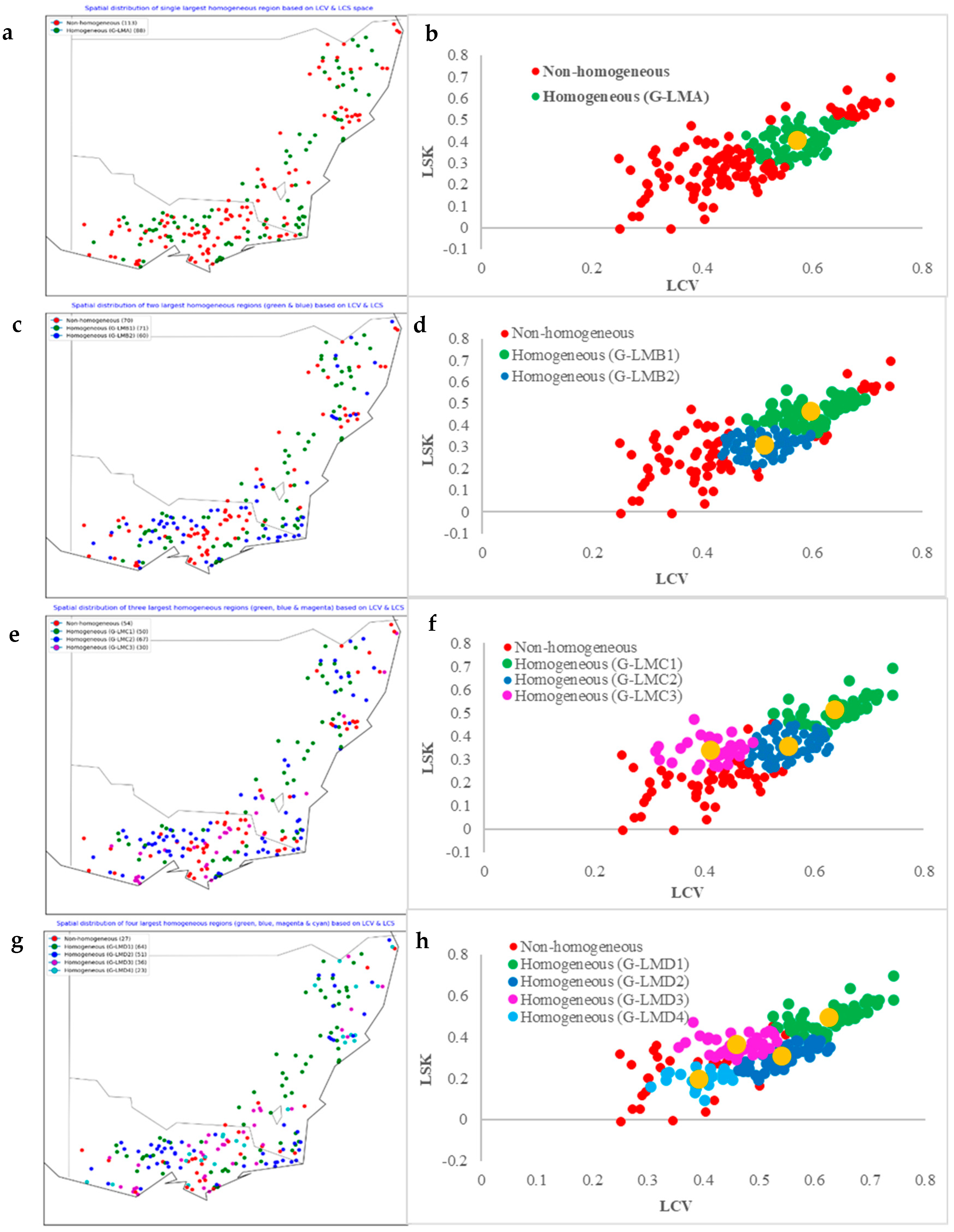
3.4. Coherence of Group Formation Between Flood Data and Catchment Data Space

Principal component analysis (PCA) and cluster analysis were performed for the sites (comprising the four largest homogeneous regions based on L-moments (of AMF data) space, n = 174). Physical and geographical coherence of groupings between the L-moments space and catchment data space is examined here. Figure 10 shows the group formation adopting PCA, Ward’s method, and K-means clustering. The scatter plot between the PC1 and PC2 space, Ward’s cluster dendrogram, and K-means clustering are shown in Figure 10 under a, b, and c, respectively. In Figure 10a, the numerals (1, 2, 3, and 4) refer to L-moments space grouping number, like G-LMD1 = 1, G-LMD2 = 2, G-LMD3, = 3, and G-LMD4 = 4. This figure evidently shows that the member sites in group G-LMD1 are distributed throughout the PC1 and PC2 space. Similarly, the member sites in groups G-LMD2, G-LMD3, and G-LMD4 are also distributed all over the PC1-PC2 space. Likewise, in the cluster dendrogram (Figure 10b,c) member sites from the L-moments grouping are allocated over the group formed based on cluster analysis (both Ward’s method and K-means clustering). The agreement of group formation was further examined by preparing scatter plots for L-moments of member sites for respective groups obtained from PCA and cluster analysis. Figure 11 shows the allocation of the sites based on L-moments coefficient. Member sites of G-LMD1 (green color) based on the L-moments space were allocated in a scattered way among the group based on PCA. However, few of these members formed a pocket in cluster analysis. Similarly, member sites of other groups (G-LMD2, G-LMD3, and G-LMD4) show the agreement of group formation to some extent in cluster analysis, but PCA does not. Hence, no significant agreement of group formation was found among the flood data/L-moments space, PCA, and cluster analysis (Ward’s method and K-means clustering).

Table 4. Agreement of group formation between L-moments space and multivariate statistical techniques (PCA, Ward’s method, and K-means clustering). The bold faced refers the highest agreement among the assumed regions.

Comparison in % (n)		LCV-LSK Space [% (n)]				Total (n)
		G-LMD1	G-LMD2	G-LMD3	G-LMD4
PC1 vs. PC2 space	QR1	25 (16)	19.61 (10)	19.44 (7)	0 (0)	33
	QR2	26.56 (17)	21.57 (11)	8.33 (3)	65.22 (15)	46
	QR3	25 (16)	29.41 (15)	38.89 (14)	34.78 (8)	53
	QR4	23.44 (15)	29.41 (15)	33.33 (12)	0 (0)	42
Ward’s Method	WMR1	9.38 (6)	17.65 (9)	0 (0)	0 (0)	15
	WMR2	18.75 (12)	9.8 (5)	11.11 (4)	78.26 (18)	39
	WMR3	21.88 (14)	29.41 (15)	47.22 (17)	17.39 (4)	50
	WMR4	50 (32)	43.14 (22)	41.67 (15)	4.35 (1)	70
K-means clustering	KMR1	9.38 (6)	17.65 (9)	0 (0)	0 (0)	15
	KMR2	40.63 (26)	37.25 (19)	38.89 (14)	0 (0)	59
	KMR3	18.75 (12)	11.76 (6)	11.11 (4)	82.61 (19)	41
	KMR4	31.25 (20)	33.33 (17)	50 (18)	17.39 (4)	59
Total		100 (64)	100 (51)	100 (36)	100 (23)	174

summarizes the degree of agreement of group formation using the L-moments space and multiple regression as explained above. It clearly describes that only 16 (25%) out of 64 member sites are common in group 1 both in the L-moments space (G-LMD1) and PCA (QR1). In group G-LMD2 vs. QR2, it is 11 (21.57%). Unfortunately, no member sites are not common in G-LMD4 vs. QR4. Considering the same group number between the L-moments space and PCA and cluster analysis, the percentage of highest (47.22%, n = 17 out of 23) agreement is found in G-LMD3 vs. WMR3, followed by G-LMD3 vs. QR3 (38.89%, n = 14 out of 23). In other words, the agreement of group formation based on flood data/the L-moments space and either of the adopted cluster analysis is highest in G-LMD4 vs. KMR3 (82.61%, n = 19 out of 23) followed by G-LMD4 vs. WMR2 (78.26%, n = 18 out of 23). These findings obviously support the graphical presentation in Figure 10 and Figure 11.

Figure 12 illustrates the comparison of principal component scores (both PC1 and PC2) obtained from each group using the selected predictors (standardized). The upper row refers to the homogeneous regions and the lower one refers to heterogeneous regions. The boxplots of PC1 for the majority of the homogeneous regions (except G-LMC1, GLMC2, and G-LMD4) show that the median (second quartile) values deviate far away from the unbiased line (“0” line). For PC2 (except G-LMA, G-LMB1, G-LMC1, and GLMC2), the deviation is far away from the ”0” line. Moreover, in the heterogeneous regions this deviation is nearly the same for PC2 but a bit better for PC1. Thus, it can be said that the degree of homogeneity does not have any impact on principal component scores.

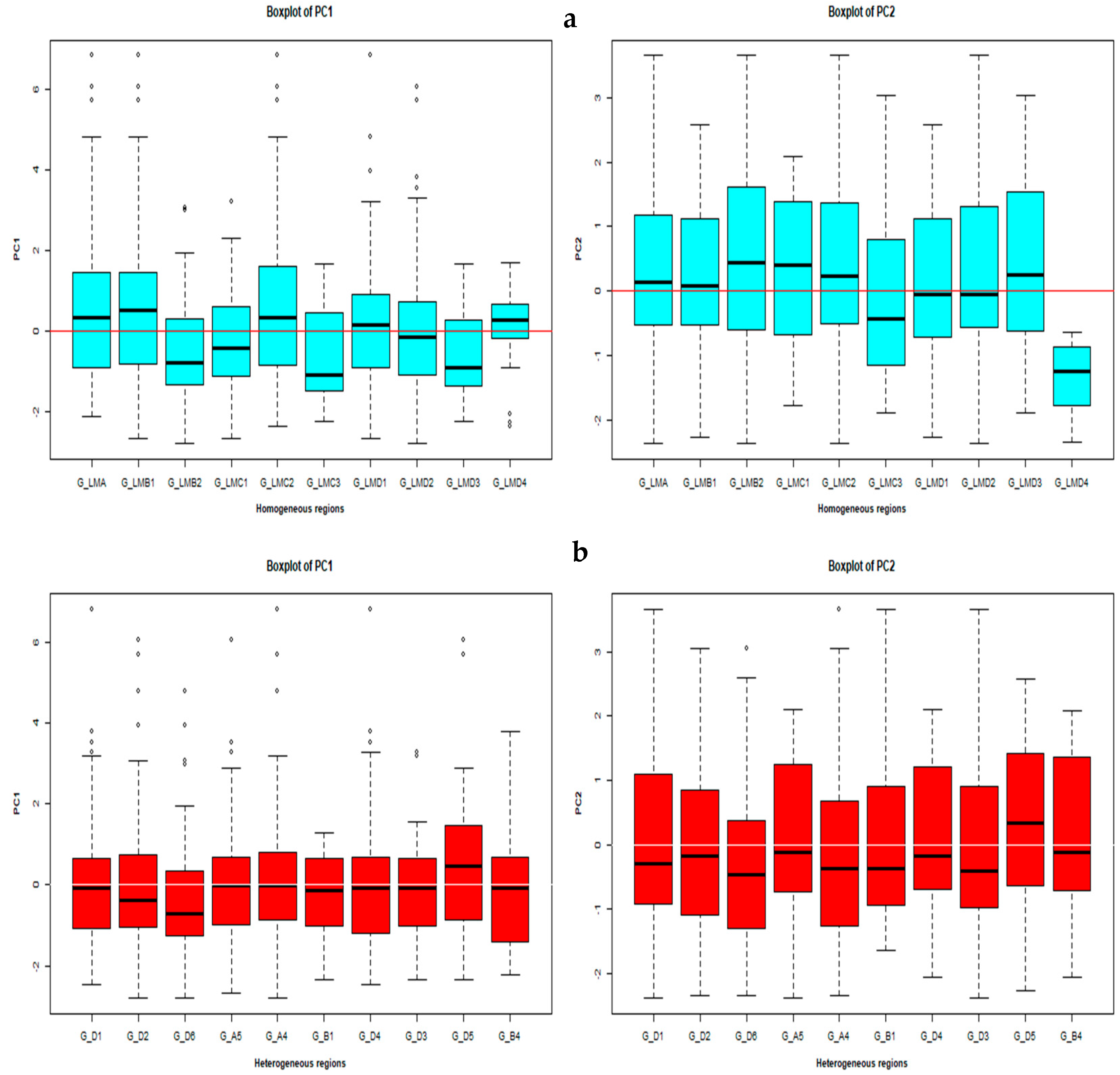
3.5. Physical and Geographical Interpretation in Terms of Degree of Homogeneity and Heterogeneity

Boxplots were created for the catchment characteristics (including LCV and LSK) to examine the physical and geographical coherence of the assumed regions (homogeneous vs. heterogeneous). In addition, spatial distributions are also presented, creating maps only for the sites comprising of the four largest homogeneous regions (L-moments space).

3.5.1. Physical Interpretation of Catchment Characteristics

Figure 13 shows the distribution of catchment characteristics and L-moments for the assumed regions (both homogeneous and heterogeneous). The first and third (left-right) columns refer to the boxplots of homogeneous regions, and the second and fourth columns refer to the boxplots for heterogenous regions with specific predictors. Among all the homogeneous regions, AREA value fluctuated roughly at a moderate variation, whereas in the heterogeneous regions this variation is high. For instance, in G-A5 the median value of AREA is away from the median values in homogeneous regions. Similar variation pattern exists between homogeneous and heterogeneous regions for I₆₂, MAR, MAE, and SDEN. Surprisingly, roughly closer variation shows for SF and S1085 between the homogeneous and heterogeneous regions. No uniform pattern is observed for FOREST value within the two types of regions. Interestingly, the values of both the LCV and LSK are nearly close to its median value within the group, but the median values are different between groups. This happens as the regions are formed based on the LCV and LSK space. On the other hand, the median values of LCV and LSK are nearly closer among the heterogeneous regions, but variation of values exists within the regions.

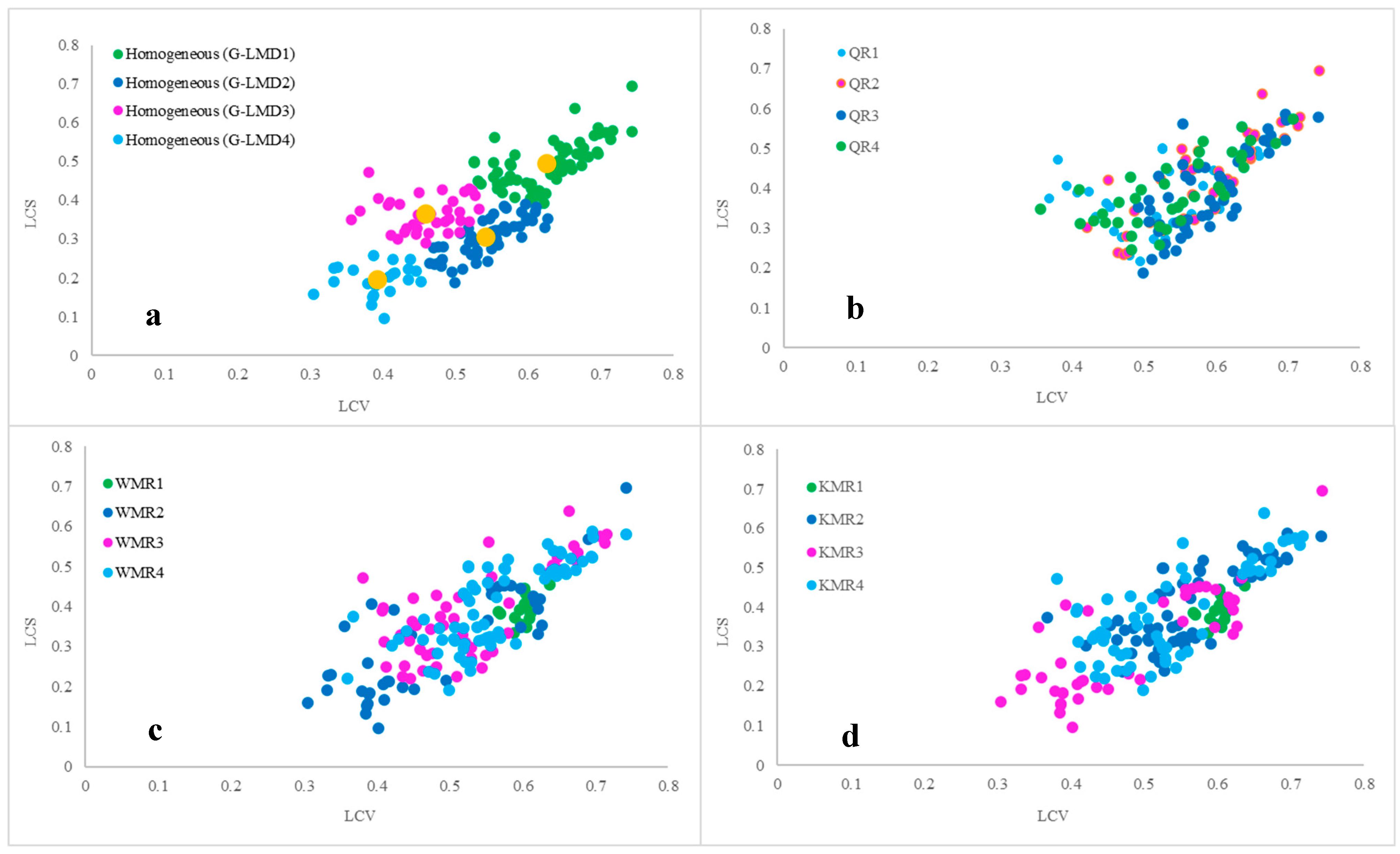
3.5.2. Geographical Coherence of Assumed Homogeneous Regions

Figure 14 shows the spatial distribution (left side) and LCV-LSK space scatter plots (right-side) for the homogeneous regions formed based on the L-moments space. The panels (top to bottom) 1st, 2nd, 3rd, and 4th refer to the distribution for the single (Figure 14a,b), two (Figure 14c,d), three (Figure 14e,f), and four (Figure 14g,h) largest homogeneous regions based on the LCV-LSK space. The 1st panel clearly indicates that the sites in a single homogeneous region (green color) are distributed over the study area with some minor pockets with fewer number of sites. Similarly, the 2nd, 3rd, and 4th panes also reveal the scatteredness of sites throughout the study area having few pockets with a smaller number of sites. These spatial distribution of sites for each region obviously indicate that homogeneous regions (formed in the L-moments space) are not geographically contiguous, which is similar to the findings of the study by Bates et al. [22].

4. Discussion

In searching for homogeneous regions in southeast Australia, regions were formed based on AREA, drainage division, basin neighborhood, and the L-moments (LCV-LSK) space. Only in the L-moments space, homogeneous regions were found and the spatial distribution (see Figure 14) for the member sites of the four largest homogeneous regions (n = 174) obviously indicates that the sites of each region are not geographically contiguous. Bates et al. [22] suggested that grouping based on the L-moments space would not show any notable pattern or trend, just reflect the noise in data, but no physical significance [16]. Among these 174 sites, multivariate statistical techniques (PCA, Ward’s method, and K-means clustering) were applied in the delineation of homogeneous regions. Though the first five PCs explain almost 89% of data variation ([31] showed 85%), no significant agreement of group formation was found (see Figure 11 and Table 4).

Taylor et al. [29] suggested, that along with other RFFA techniques, the QRT and IFM are commonly used for regional flood estimation. Though the QRT relaxes the homogeneity assumptions, the IFM requires ‘acceptably regional homogeneity’ [16], which is hard to find in Australia [22]. Adopting the QRT, the estimated AMRE values range from 28% to 79% [29]. In Western Australia (Pilbara), a study adopted the IFM using ordinary least square and found that AMRE values ranged from 23% to 46% (Q₂ to Q₁₀₀) for streamflow data [63]. The present study found reasonably comparable result adopting the IFM and QRT using the member sites of four largest L-moments based regions. Over the quantiles (Q₂ to Q₁₀₀), the AMRE values range from 32.45% to 62.98% for the IFM (see Table 3) and 27.98% to 54.34% for the QRT (see Table 2). It indicates that overall, the QRT outperforms the IFM in southeast Australia. Using 202 sites from Australia, adopting network theory and commonly used models to estimate flood quantiles, the estimated RMSE values range from 23% (Q₂) to 29% (Q₁₀₀) [19]. In a study in Australia, Rahman et al. [27] adopted independent component analysis integrating with the QRT to estimate flood quantiles. The evaluation criteria AMRE and RMSNE were estimated, which ranged from 33.28% to 43.92% and 0.95 to 3.60 over the different return periods [27].

In a study in India, classical RFFA method and deep-learning (DL) approach (Random Forest—RF and eXtreme Gradient Boosting—XGBoost) were applied for annual maximum streamflow data in a data sparse region. The study found that the AMRE and RMSE values could be reduced by roughly 50% by using a DL approach rather than the classical RFFA method with a higher R² (0.85 to 0.96) [6]. In a study in Iran, using 32 gauged sites to delineate homogeneous regions, Ward’s method was applied, which resulted in two regions. The Z-statistic concluded that GLO and GPA were the best fit distributions for the first and second region, respectively. Adopting the IFM and multiple regression among these two regions, the estimated RRMSE values fluctuated from 0.995 to 3.674 and 1.002 to 5.692, respectively [61]. A similar study in Iran estimated RRMSE for the IFM and multiple linear regression, which were found to vary from 0.23 to 0.36, and 0.29 to 0.53, respectively [34].

In Turkey (West Mediterranean River basin), a study conducted for model evaluation used 47 gauged sites integrating with IFM and L-moments parameters. The estimated values for BIAS ranged nearly from −0.2 to 0.6 and for RRMSE it ranged roughly from 0.15 to 0.60 [64]. Similarly, in another study in Turkey to evaluate the quantile estimates the RMSE, BIAS, and RBIAS were reported; over the quantiles, these reported values ranged from 0.037 to 0.247, 0.002 to 0.022, and 0.124 to 0.205, respectively. Based on multiple linear regression analysis using data from all over the world (excluding Australia), the reported RMSNE values ranged from 0.50 to 0.65 [65]. Tramblay et al. [66] developed a RFFA for Northern Africa and noted that Lasso regression provided mean absolute relative errors close to 50% [66]. Singh and Chavan (2025) applied region-of-influence approach to form regions in the USA and India and found that nearly 20% of the formed regions had an H₁ measure less than 2 [67]. The RRMSE values of the proposed RFFA were 33.33 and 54.56 for the USA and India, respectively. Desai and Ouarda (2021) conducted RFFA in southern Quebec, Canada using a random forest regression and noted a BIAS value of −0.019 for a 100-year return period [68].

Australia is a country of highly variable hydrology, especially southeast Australia. With highly heterogeneous regions, the findings of this study are comparable with various domestic and international RFFA studies. For instance, in terms of AMRE values the findings from Taylor et al. [29], Haque et al. [63], and Rahman et al. [27] are comparable to those from this study. The estimated AMRE values are comparable with the findings of Australian Rainfall and Runoff (ARR), which ranged from 57.25 to 64.06% [28,69,70]. Though the RRMSE (ranges from 0.14 to 0.61 for the IFM and 0.00 to 0.35 for the QRT) and RMSNE (0.43 to 1.33 for the IFM and 0.48 to 2.37 for the QRT) values are almost similar ti other study findings, the MSE and RMSE values are higher in this study. This might be due to high variation in hydro-climatic parameters across different catchments. The heterogeneity in a region has little influence on the model accuracy in regional flood quantile estimation. Alexandre et al. [71] reported that application of a Bayesian hierarchical model based on Generalized Extreme Value (GEV) distribution could provide accurate flood quantile estimates (median relative error of 19%) despite a marked regional heterogeneity across North America [71]. This shows that there are RFFA methods that are not dependent on homogeneous regions.

This study used streamflow data from 201 stations, which have different record lengths (25 to 89 years). It should be noted that shorter streamflow record length introduces sampling variability affecting L-moment estimates, which has introduced uncertainty in the results. Also, AMF data of nearby stations are generally correlated, which has affected accuracy of the LOO validation technique.

5. Conclusions

This study investigates homogeneous region identification in the context of RFFA in southeast Australia. Regions were formed based on catchment size, drainage division, basin contiguity, and the L-moments (of AMF data) space. In addition, a comparison between the QRT and IFM was conducted to estimate flood quantiles for the four homogeneous regions formed in the L-moments space. Hosking and Wallis [16] test criteria were used to test the discordancy of sites and heterogeneity of the assumed regions. Considering all the assumed regions and a LOO validation technique, the estimated AMRE values range was 20.01–77.27%. However, for the four L-moments-based homogeneous regions, these values range from 27.98–54.34% for the QRT, and 32.45–62.98% for the IFM. The major findings of this study are noted below:

• The Pearson Type III (PE3) and Generalized Pareto (GPA) distributions are the best-fit regional distributions in southeast Australia.
• For the homogeneous regions (formed in the L-moments space), the variation in estimated model accuracy is smaller for the IFM than the QRT, but the QRT generally outperforms the IFM with lower AMRE values.
• There is a weak association between the flood characteristics data space (L-moments of AMF data) and catchment characteristics data space in southeast Australia.

The limitations of this study include a smaller data set is used consisting of only 201 stations from a large area of southeast Australia. Also, AMF data length of some of the selected stations are small (25 years), which introduced a greater sampling variability in the estimates of L-moments of the AMF data and other flood statistics. Future studies should focus on the application of a parameter regression technique instead of the QRT and impacts of climate change on regional homogeneity.

References

1. Endendijk, T.; Botzen, W.; de Moel, H.; Aerts, J.; Slager, K.; Kok, M. Flood Vulnerability curves and household flood damage mitigation measures: An econometric analysis of survey data. In Proceedings of the EGU23, the 25th EGU General Assembly, Vienna, Austria, 23–28 April 2023. Copernicus Meetings. [Google Scholar]
2. FitzGerald, G.; Du, W.; Jamal, A.; Clark, M.; Hou, X.Y. Flood fatalities in contemporary Australia (1997–2008). Emerg. Med. Australas. 2010, 22, 180–186. [Google Scholar] [CrossRef]
3. Li, Z.; Gao, S.; Chen, M.; Gourley, J.J.; Hong, Y. Spatiotemporal characteristics of US floods: Current status and forecast under a future warmer climate. Earth’s Future 2022, 10, e2022EF002700. [Google Scholar] [CrossRef]
4. Rhodes, C. Flood Damage Costs Beyond Buildings—A Lake Champlain Case Study; US Geological Survey: Reston, VA, USA, 2023. [Google Scholar]
5. Quesada-Román, A.; Ballesteros-Cánovas, J.A.; Granados-Bolaños, S.; Birkel, C.; Stoffel, M. Improving regional flood risk assessment using flood frequency and dendrogeomorphic analyses in mountain catchments impacted by tropical cyclones. Geomorphology 2022, 396, 108000. [Google Scholar] [CrossRef]
6. Mangukiya, N.K.; Sharma, A. Alternate pathway for regional flood frequency analysis in data-sparse region. J. Hydrol. 2024, 629, 130635. [Google Scholar] [CrossRef]
7. Sharifi Garmdareh, E.; Vafakhah, M.; Eslamian, S.S. Regional flood frequency analysis using support vector regression in arid and semi-arid regions of Iran. Hydrol. Sci. J. 2018, 63, 426–440. [Google Scholar] [CrossRef]
8. Srinivas, V.V.; Tripathi, S.; Rao, A.R.; Govindaraju, R.S. Regional flood frequency analysis by combining self-organizing feature map and fuzzy clustering. J. Hydrol. 2008, 348, 148–166. [Google Scholar] [CrossRef]
9. Stedinger, J.R.; Griffis, V.W. Flood frequency analysis in the United States: Time to update. J. Hydrol. Eng. 2008, 13, 199–204. [Google Scholar] [CrossRef]
10. Kumar, R.; Goel, N.K.; Chatterjee, C.; Nayak, P.C. Regional flood frequency analysis using soft computing techniques. Water Resour. Manag. 2015, 29, 1965–1978. [Google Scholar] [CrossRef]
11. Mengistu, T.D.; Feyissa, T.A.; Chung, I.M.; Chang, S.W.; Yesuf, M.B.; Alemayehu, E. Regional Flood Frequency Analysis for Sustainable Water Resources Management of Genale–Dawa River Basin, Ethiopia. Water 2022, 14, 637. [Google Scholar] [CrossRef]
12. Ouarda, T.B.; Girard, C.; Cavadias, G.S.; Bobée, B. Regional flood frequency estimation with canonical correlation analysis. J. Hydrol. 2001, 254, 157–173. [Google Scholar] [CrossRef]
13. Ouarda, T.B.; Bâ, K.M.; Diaz-Delgado, C.; Cârsteanu, A.; Chokmani, K.; Gingras, H.; Quentin, E.; Trujillo, E.; Bobée, B. Intercomparison of regional flood frequency estimation methods at ungauged sites for a Mexican case study. J. Hydrol. 2008, 348, 40–58. [Google Scholar] [CrossRef]
14. Guru, N. Implication of partial duration series on regional flood frequency analysis. Int. J. River Basin Manag. 2024, 22, 167–186. [Google Scholar] [CrossRef]
15. Dalrymple, T. Flood-Frequency Analyses, Manual of Hydrology: Part 3; USGPO: Washington, DC, USA, 1960. [Google Scholar]
16. Hosking, J.R.M.; Wallis, J.R. Some statistics useful in regional frequency analysis. Water Resour. Res. 1993, 29, 271–281. [Google Scholar] [CrossRef]
17. Griffis, V.; Stedinger, J. The use of GLS regression in regional hydrologic analyses. J. Hydrol. 2007, 344, 82–95. [Google Scholar] [CrossRef]
18. Mostofi Zadeh, S.; Burn, D.H. A Super Region Approach to Improve Pooled Flood Frequency Analysis. Can. Water Resour. J./Rev. Can. Des Ressour. Hydr. 2019, 44, 146–159. [Google Scholar] [CrossRef]
19. Han, X.; Ouarda, T.B.M.J.; Rahman, A.; Haddad, K.; Mehrotra, R.; Sharma, A. A Network Approach for Delineating Homogeneous Regions in Regional Flood Frequency Analysis. Water Resour. Res. 2020, 56, e2019WR025910. [Google Scholar] [CrossRef]
20. Burn, D.H. Delineation of groups for regional flood frequency analysis. J. Hydrol. 1988, 104, 345–361. [Google Scholar] [CrossRef]
21. Viglione, A.; Laio, F.; Claps, P. A comparison of homogeneity tests for regional frequency analysis. Water Resour. Res. 2007, 43. [Google Scholar] [CrossRef]
22. Bates, B.C.; Rahman, A.; Mein, R.G.; Weinmann, P.E. Climatic and physical factors that influence the homogeneity of regional floods in southeastern Australia. Water Resour. Res. 1998, 34, 3369–3381. [Google Scholar] [CrossRef]
23. Sabrina, A.; Rahman, A. Development of a kriging-based regional flood frequency analysis technique for South-East Australia. Nat. Hazards 2022, 114, 2739–2765. [Google Scholar]
24. Zalnezhad, A.; Rahman, A.; Vafakhah, M.; Samali, B.; Ahamed, F. Regional Flood Frequency Analysis Using the FCM-ANFIS Algorithm: A Case Study in South-Eastern Australia. Water 2022, 14, 1608. [Google Scholar] [CrossRef]
25. Ahmed, A.; Khan, Z.; Rahman, A. Searching for homogeneous regions in regional flood frequency analysis for Southeast Australia. J. Hydrol. Reg. Stud. 2024, 53, 101782. [Google Scholar] [CrossRef]
26. Rahman, A. Flood Estimation for Ungauged Catchments: A Regional Approach using Flood and Catchment Characteristics. Ph.D. Thesis, Department of Civil Engineering, Monash University, Victoria, Australia, 1997. [Google Scholar]
27. Rahman, A.S.; Khan, Z.; Rahman, A. Application of independent component analysis in regional flood frequency analysis: Comparison between quantile regression and parameter regression techniques. J. Hydrol. 2020, 581, 124372. [Google Scholar] [CrossRef]
28. Rahman, A.; Haddad, K.; Kuczera, G.; Weinmann, E. Regional Flood Methods. In Australian Rainfall and Runoff: A Guide to Flood Estimation; Chapter 3, Book 3; Ball J, B.M., Nathan, R., Weeks, W., Weinmann, E., Retallick, M., Testoni, I., Eds.; Geoscience Australia, Commonwealth of Australia, Engineers Australia: Symonston, Australia, 2019. [Google Scholar]
29. Taylor, M.; Haddad, K.; Zaman, M.; Rahman, A. Regional flood modelling in Western Australia: Application of regression based methods using ordinary least squares. In Proceedings of the 19th International Congress on Modelling and Simulation—Sustaining Our Future: Understanding and Living with Uncertainty, MODSIM2011, Perth, WA, USA, 12–16 December 2011; pp. 3803–3810. [Google Scholar]
30. Zalnezhad, A.; Rahman, A.; Nasiri, N.; Haddad, K.; Rahman, M.M.; Vafakhah, M.; Samali, B.; Ahamed, F. Artificial Intelligence-Based Regional Flood Frequency Analysis Methods: A Scoping Review. Water 2022, 14, 2677. [Google Scholar] [CrossRef]
31. Rahman, A.S.; Rahman, A. Application of Principal Component Analysis and Cluster Analysis in Regional Flood Frequency Analysis: A Case Study in New South Wales, Australia. Water 2020, 12, 781. [Google Scholar] [CrossRef]
32. Gado, T.A.; Nguyen, V.T.V. Comparison of homogenous region delineation approaches for regional flood frequency analysis at ungauged sites. J. Hydrol. Eng. 2016, 21. [Google Scholar] [CrossRef]
33. Ward Jr, J.H. Hierarchical grouping to optimize an objective function. J. Am. Stat. Assoc. 1963, 58, 236–244. [Google Scholar] [CrossRef]
34. Malekinezhad, H.; Nachtnebel, H.P.; Klik, A. Comparing the index-flood and multiple-regression methods using L-moments. Phys. Chem. Earth Parts A/B/C 2011, 36, 54–60. [Google Scholar] [CrossRef]
35. Murtagh, F.; Legendre, P. Ward’s hierarchical agglomerative clustering method: Which algorithms implement Ward’s criterion? J. Classif. 2014, 31, 274–295. [Google Scholar] [CrossRef]
36. Farsadnia, F.; Rostami Kamrood, M.; Moghaddam Nia, A.; Modarres, R.; Bray, M.T.; Han, D.; Sadatinejad, J. Identification of homogeneous regions for regionalization of watersheds by two-level self-organizing feature maps. J. Hydrol. 2014, 509, 387–397. [Google Scholar] [CrossRef]
37. Sharghi, E.; Nourani, V.; Soleimani, S.; Sadikoglu, F. Application of different clustering approaches to hydroclimatological catchment regionalization in mountainous regions, a case study in Utah State. J. Mt. Sci. 2018, 15, 461–484. [Google Scholar] [CrossRef]
38. Acreman, M.C.; Sinclair, C.D. Classification of drainage basins according to their physical characteristics; an application for flood frequency analysis in Scotland. J. Hydrol. 1986, 84, 365–380. [Google Scholar] [CrossRef]
39. Ahani, A.; Mousavi Nadoushani, S.S.; Moridi, A. A ranking method for regionalization of watersheds. J. Hydrol. 2022, 609, 127740. [Google Scholar] [CrossRef]
40. Zhang, R.; Chen, Y.; Zhang, X.; Ma, Q.; Ren, L. Mapping homogeneous regions for flash floods using machine learning: A case study in Jiangxi province, China. Int. J. Appl. Earth Obs. Geoinf. 2022, 108, 102717. [Google Scholar] [CrossRef]
41. Baidya, S.; Singh, A.; Panda, S.N. Flood frequency analysis. Nat. Hazards 2020, 100, 1137–1158. [Google Scholar] [CrossRef]
42. Kuczera, G. Comprehensive at-site flood frequency analysis using Monte Carlo Bayesian inference. Water Resour. Res. 1999, 35, 1551–1557. [Google Scholar] [CrossRef]
43. Kuczera, G.; Franks, S.W. At-Site Flood Frequency Analysis. In Australian Rainfall and Runoff: A Guide to Flood Estimation; Chapter 3, Book 3; Ball J, B.M., Nathan, R., Weeks, W., Weinmann, E., Retallick, M., Testoni, I., Eds.; Geoscience Australia: Symonston, Australia, 2019. [Google Scholar]
44. Franks, S.W.; Kuczera, G. Flood frequency analysis: Evidence and implications of secular climate variability, New South Wales. Water Resour. Res. 2002, 38, 20-21–20-27. [Google Scholar] [CrossRef]
45. Rahman, A.S.; Rahman, A.; Zaman, M.A.; Haddad, K.; Ahsan, A.; Imteaz, M. A study on selection of probability distributions for at-site flood frequency analysis in Australia. Nat. Hazards 2013, 69, 1803–1813. [Google Scholar] [CrossRef]
46. Bobée, B.; Mathier, L.; Perron, H.; Trudel, P.; Rasmussen, P.F.; Cavadias, G.; Bernier, J.; Nguyen, V.T.V.; Pandey, G.; Ashkar, F.; et al. Presentation and review of some methods for regional flood frequency analysis. J. Hydrol. 1996, 186, 63–84. [Google Scholar]
47. Rahman, A. A quantile regression technique to estimate design floods for ungauged catchments in south-east Australia. Australas. J. Water Resour. 2005, 9, 81–89. [Google Scholar] [CrossRef]
48. Rahman, A.; Haddad, K.; Zaman, M.; Kuczera, G.; Weinmann, P.E. Design Flood Estimation in Ungauged Catchments: A Comparison Between the Probabilistic Rational Method and Quantile Regression Technique for NSW. Australas. J. Water Resour. 2011, 14, 127–139. [Google Scholar] [CrossRef]
49. Thomas, D.; Benson, M.A. Generalization of Streamflow Characteristics from Drainage-Basin Characteristics; US Government Printing Office: Washington, DC, USA, 1970. [Google Scholar]
50. Hosking, J.R.M.; Wallis, J.R. Regional Frequency Analysis: An Approach Based on L-Moments; Cambridge University Press: New York, NY, USA, 1997. [Google Scholar]
51. Ouarda, T.B.M.J. Handbook of Applied Hydrology, Second Edition, Chapter 77, Regional Flood Frequency Modeling; Regional Flood Frequency Modeling, ed. V.P.S. (Editor-in-Chief); McGraw-Hill Education: New York, NY, USA, 2017. [Google Scholar]
52. Cunnane, C. Methods and merits of regional flood frequency analysis. J. Hydrol. 1988, 100, 269–290. [Google Scholar] [CrossRef]
53. Potter, K.W.; Lettenmaier, D.P. A comparison of regional flood frequency estimation methods using a resampling method. Water Resour. Res. 1990, 26, 415–424. [Google Scholar] [CrossRef]
54. GREH, G.D.R.E.H.S. Inter-comparison of regional flood frequency procedures for Canadian rivers. J. Hydrol. 1996, 186, 85–103. [Google Scholar]
55. Aissia, B.; Chebana, F.; Ouarda, T.; Bruneau, P.; Barbet, M.; Équipement, H.-Q. Bivariate index flood model for a northern case study. Hydrol. Sci. J. 2015, 60, 247–268. [Google Scholar] [CrossRef]
56. Chebana, F.; Ouarda, T.B. Index flood-based multivariate regional frequency analysis. Water Resour. Res. 2009, 45. [Google Scholar] [CrossRef]
57. Formetta, G.; Over, T.; Stewart, E. Assessment of Peak Flow Scaling and Its Effect on Flood Quantile Estimation in the United Kingdom. Water Resour. Res. 2021, 57, e2020WR028076. [Google Scholar] [CrossRef]
58. Kader, F.; Derbas, A.; Haddad, K.; Rahman, A. Regional flood estimation for NSW: Comparison of quantile regression and parameter regression techniques. In Proceedings of the 21st International Congress on Modelling and Simulation: Partnering with Industry and the Community for Innovation and Impact through Modelling, MODSIM 2015—Held jointly with the 23rd National Conference of the Australian Society for Operations Research and the DSTO Led Defence Operations Research Symposium, DORS 2015, Queensland, Australia, 29 November–4 December 2015; Modelling and Simulation Society of Australia and New Zealand Inc. (MSSANZ): Perth, WA, Australia, 2015; pp. 2179–2185. [Google Scholar]
59. Requena, A.I.; Chebana, F.; Mediero, L. A complete procedure for multivariate index-flood model application. J. Hydrol. 2016, 535, 559–580. [Google Scholar] [CrossRef]
60. Šimková, T. L-moment homogeneity test in trivariate regional frequency analysis of extreme precipitation events. Meteorol. Appl. 2018, 25, 11–22. [Google Scholar] [CrossRef]
61. Mosaffaie, J. Comparison of two methods of regional flood frequency analysis by using L-moments. Water Resour. 2015, 42, 313–321. [Google Scholar] [CrossRef]
62. Haddad, K.; Rahman, A.; A Zaman, M.; Shrestha, S. Applicability of Monte Carlo cross validation technique for model development and validation using generalised least squares regression. J. Hydrol. 2013, 482, 119–128. [Google Scholar] [CrossRef]
63. Haque, M.M.; Rahman, A.; Haddad, K.; Kuczera, G.; Weeks, W. Development of a regional flood frequency estimation model for Pilbara, Australia. In Proceedings of the 21st International Congress on Modelling and Simulation: Partnering with Industry and the Community for Innovation and Impact through Modelling, MODSIM 2015—Held jointly with the 23rd National Conference of the Australian Society for Operations Research and the DSTO led Defence Operations Research Symposium, DORS 2015, Queensland, Australia, 29 November–4 December 2015; Modelling and Simulation Society of Australia and New Zealand Inc. (MSSANZ): Perth, WA, Australia, 2015; pp. 2172–2178. [Google Scholar]
64. Saf, B. Regional Flood Frequency Analysis Using L-Moments for the West Mediterranean Region of Turkey. Water Resour. Manag. 2008, 23, 531–551. [Google Scholar] [CrossRef]
65. Rosbjerg, D.; Bloschl, G.; Burn, D.; Castellarin, A.; Croke, B.; Di Baldassarre, G.; Iacobellis, V.; Kjeldsen, T.R.; Kuczera, G.; Merz, R. Prediction of floods in ungauged basins. In Runoff Prediction in Ungauged Basins: Synthesis Across Processes, Places and Scales; Cambridge University Press: Cambridge, UK, 2013; pp. 189–225. [Google Scholar]
66. Tramblay, Y.; Khedimallah, A.; Sadaoui, M.; Benaabidate, L.; Boulmaiz, T.; Boutaghane, H.; Dakhlaoui, H.; Hanich, L.; Ludwig, W.; Meddi, M. Regional flood frequency analysis in North Africa. J. Hydrol. 2024, 630, 130678. [Google Scholar] [CrossRef]
67. Singh, A.K.; Chavan, S.R. An approach to regional flood frequency analysis for general peak discharge distribution datasets. J. Hydrol. 2025, 650, 132493. [Google Scholar] [CrossRef]
68. Desai, S.; Ouarda, T.B. Regional hydrological frequency analysis at ungauged sites with random forest regression. J. Hydrol. 2021, 594, 125861. [Google Scholar] [CrossRef]
69. Rahman, A.; Haddad, K.; Rahman, A.S.; Haque, M. Australian Rainfall and Runoff Revision Project 5: Regional Flood Methods: Database Used to Develop ARR RFFE Technique: Stage 3 Report; Engineers Australia: Barton, Australia, 2015. [Google Scholar]
70. Haddad, K.; Rahman, A. Regional flood frequency analysis in eastern Australia: Bayesian GLS regression-based methods within fixed region and ROI framework—Quantile Regression vs. Parameter Regression Technique. J. Hydrol. 2012, 430–431, 142–161. [Google Scholar] [CrossRef]
71. Alexandre, D.A.; Chaudhuri, C.; Gill-Fortin, J. Continental Scale Regional Flood Frequency Analysis: Combining Enhanced Datasets and a Bayesian Framework. Hydrology 2024, 11, 119. [Google Scholar] [CrossRef]
Figure 1. Flow chart illustrating the adopted methodology.
Water 17 01799 g001
Figure 2. Location of selected stream gauging stations in southeast Australia (n = 201). Each red dot refers to a stream gauging station.
Water 17 01799 g002
Figure 3. Spatial distribution of selected stations by category based on AREA.
Water 17 01799 g003
Figure 4. Comparison of Hi-statistics (median) for the assumed regions in southeast Australia.
Water 17 01799 g004
Figure 5. Comparison of absolute median relative error with H1-statistics among the assumed regions in southeast Australia.
Water 17 01799 g005
Figure 6. Comparison of boxplots for RE (%) values between the assumed homogeneous and heterogeneous regions (QRT) by quantiles.
Water 17 01799 g006
Figure 7. Comparison of standardized flood frequency curves for six quantiles between the four largest homogeneous regions (vertical left column) based on the LCV-LSK space and heterogeneous regions (vertical right column). Each line refers to a standardized flood frequency curve for a station.
Water 17 01799 g007
Figure 8. Comparison of estimated absolute median RE (%) values from the developed model adopted by the QRT and IFM.
Water 17 01799 g008
Figure 9. Comparison of RE (%) values estimated from the developed models adopting the QRT and IFM (homogeneous regions).
Water 17 01799 g009
Figure 10. Comparison of group formation adopting (a) PCA, a scatter plot of the PC1 and PC2 space, (b) Ward’s method, and (c) K-means clustering.
Water 17 01799 g010
Figure 11. Comparison of region formation (scatter plots of L-moments coefficient for respective group member sites) adopting (a) LCV-LSK space, (b) PCA, (c) Ward’s method, and (d) K-means clustering. Each colour represents a group of catchments.
Water 17 01799 g011
Figure 12. Comparison of PC1 and PC2 between (a) L-moments-based homogeneous regions and (b) Heterogeneous regions with nearly same number of sites in respective groups.
Water 17 01799 g012
Figure 13. Comparison boxplots of catchment characteristics values between the assumed homogeneous and heterogeneous regions.
Water 17 01799 g013
Figure 14. Comparison of region formation between spatial (left-side) and LCV-LSK space (right-side); (a,b) single largest homogeneous region, (c,d) two largest homogeneous regions, (e,f) three largest homogeneous regions, (g,h) four largest homogeneous regions. Larger yellow color circle indicates the coordinates with respect to the mean values of LCV and LSK for each region.
Water 17 01799 g014