Article

Multi-Algorithm Comparison for Water Quality Retrieval: Integrating Landsat-8 OLI and Machine Learning in Karst Plateau Reservoirs

1
Karst Research Institute, College of Geography and Environmental Sciences, Guizhou Normal University, Guiyang 550001, China
2
The State Key Laboratory Incubation Base for Karst Mountain Ecology Environment of Guizhou Province, Guiyang 550001, China
*
Author to whom correspondence should be addressed.
Water 2025, 17(12), 1781; https://doi.org/10.3390/w17121781
Submission received: 14 May 2025 / Revised: 11 June 2025 / Accepted: 12 June 2025 / Published: 13 June 2025
(This article belongs to the Section Water Quality and Contamination)

Abstract

:
Chlorophyll a (Chla), total phosphorus (TP), total nitrogen (TN), and turbidity (Turb) are key indicators for assessing water eutrophication. To overcome the limitations of conventional regression methods, this study developed and compared inversion models for these parameters using Landsat-8 OLI imagery and field data, comparing multiple linear regression and seven machine learning algorithms: Genetic Algorithm- and Particle Swarm-optimized Backpropagation Neural Networks (BPNNs), Convolutional Neural Network (CNN), Extreme Learning Machine (ELM), Random Forest (RF), XGBoost, and Support Vector Regression (SVR). The results revealed that traditional regression performed better for optically active parameters (Chla and Turb) than for non-optically active ones (TP and TN), whereas machine learning models significantly improved accuracy, particularly for TP and TN. The XGBoost model achieved the highest performance (R2 > 0.90 for all parameters). Post-calibration analysis further delineated the spatial distributions and inter-parameter correlations in Pingzhai Reservoir, providing a robust method for water quality monitoring and assessment.

1. Introduction

Water resources are fundamental to human survival and socioeconomic development, serving as a critical natural asset. Rapid urbanization and population growth have led to a surge in industrial and domestic water demand [1], resulting in concurrent water pollution and scarcity that increasingly threaten water security and sustainable development. Consequently, systematic monitoring of aquatic ecosystems (lakes and rivers) is imperative [2]. Advancing monitoring technologies to improve efficiency and accuracy is critical for safeguarding water resources, mitigating pollution, and optimizing management strategies [3].
Conventional water quality monitoring relies on field sampling followed by laboratory-based physicochemical analysis. Although this approach achieves high accuracy, it suffers from low efficiency and spatial representativeness limitations, as discrete sampling points cannot adequately characterize the holistic water quality status or parameter distributions across entire water bodies [4,5,6]. In comparison, remote sensing-based water quality inversion offers macroscopic surveillance capabilities, enabling (1) basin-scale parameter mapping across temporal scales, (2) compensation for spatiotemporal discontinuities inherent to traditional methods, and (3) dynamic monitoring with advantages in temporal resolution, spatial coverage, and operational efficiency [7,8,9].
Remote sensing-based water quality monitoring has emerged as a prominent research focus globally due to its inherent advantages. Representative studies demonstrate this potential: Cruz-Retana et al. [10] achieved successful inversion of TN and TP in inland lakes using Landsat-8 multispectral imagery through multiple regression analysis. Similarly, Peng et al. [11] employed spatiotemporal ensemble modeling with Sentinel-2 data to estimate Chla, TN, and COD in Poyang Lake, while Yepez et al. [12] established a high-accuracy Turb inversion model based on Landsat-8 OLI band combinations (B4+B5). These findings collectively confirm strong correlations between key water quality parameters (Chla, TN, TP, Turb) and multispectral reflectance, validating the feasibility of remote sensing-based quantification.
The advent of artificial intelligence has further revolutionized this field, with machine learning (ML) and deep learning algorithms offering enhanced stability and accuracy for water quality estimation [7,13,14,15,16,17]. This advancement proves particularly valuable for non-optically active parameters (TP, TN, TOC, COD) whose concentration-spectra relationships are often nonlinear and influenced by complex environmental factors [18,19]. Traditional regression methods frequently fail to capture these intricate patterns, whereas ML algorithms excel at modeling such nonlinear dynamics through flexible hypothesis spaces during training [14,16,20]. Empirical evidence supports this advantage: He et al. [21] demonstrated BP neural networks’ superiority over linear regression for SD, CODMn (permanganate index), and TN estimation; Ren et al. [22] achieved nonlinear fitting of coastal water parameters using modified support vector regression; and Guo et al. [23] enhanced suspended solids inversion accuracy in the Haihe River via PSO-optimized BP networks. Although ML applications now span diverse water bodies (bays, lakes, rivers) [24,25,26], research on karst plateau lakes remains scarce. Due to their unique geomorphological features (intense dissolution, well-developed subterranean rivers) and hydrological characteristics (low flow velocity, high ion concentration), karst plateau lakes exhibit distinct optical properties compared to ordinary lakes [27]. Consequently, independent modeling is essential for remote sensing inversion of water color parameters to avoid errors caused by differences in water constituents and light field distribution. Therefore, this study conducts a comparative evaluation of multiple algorithms tailored to this distinctive hydrogeological environment.
While individual ML algorithms can improve inversion accuracy, their varying architectures lead to differential performance across water quality parameters. This study addresses this gap by (1) establishing and comparing ML-based inversion models (using Landsat-8 imagery and in situ data) for four parameters (Chla, TN, TP, and Turb) in Pingzhai Reservoir—a representative karst plateau lake in Guizhou Province; and (2) analyzing post-simulation water quality distributions and inter-parameter relationships. Our findings provide critical data and methodological references for reservoir management in karst regions while advancing technical frameworks for similar aquatic ecosystems.

2. Materials and Methods

2.1. Overview of the Study Area

As a critical water body in the karst region of Southwest China, Pingzhai Reservoir straddles the border between Liupanshui City and Bijie City in Guizhou Province, China (Figure 1). The reservoir lies within a typical karst peak-cluster depression terrain, formed by damming five tributaries: Nayong River, Zhangwei River, Shuigong River, Hujia River, and Baishui River. The Pingzhai reservoir belongs to the Beipan River system of the Pearl River Basin. Its primary recharge sources are precipitation and groundwater, with groundwater contributing 30–40% of the total inflow during dry seasons. The water quality consistently meets or exceeds drinking water standards.
The watershed spans 834.45 km2 with pronounced topographic variability, featuring elevation gradients from 1182 to 2291 m and slope angles ranging from 0 to 69°. Hydrologically, the reservoir maintains a normal storage level of 1331 m, with an average depth of 80 m and a total storage capacity of 1.089 × 10⁹ m3. The region exhibits well-developed karst landforms, including surface features such as peak-cluster depressions, sinkholes, and solution dolines, as well as subsurface systems comprising caves and interconnected karst conduits. Notably, studies confirm an extensive karst groundwater system underlying the reservoir [28,29]. As a strategic freshwater resource, this phreatic aquifer exhibits hydrochemical coupling with surface water through karst conduits. The reservoir experiences a subtropical monsoon climate characterized by a mean annual temperature of 14.0 °C and annual precipitation of 1053.5 mm, with approximately 70% of rainfall occurring between June and September.
The watershed encompasses four administrative units—Nayong County, Zhijin County, Liuzhi Special Zone, and Shuicheng County—including 11 townships, among which Zhangjiawan, Baixing, and Jichang are the most populated. Intensive agriculture and mining activities in these areas [30] contribute nutrient loads and sediments to the reservoir through both surface runoff and karst drainage networks, posing dual threats to surface and groundwater quality.

2.2. Field Measurement Data

Based on the geographic location and morphology of Pingzhai Reservoir, we deployed a total of 30 water sampling points following the principle of uniform distribution while avoiding mountain shadows (calculated using ArcGIS 10.8). Their locations are shown in Figure 1.
Sampling was conducted on 27 July 2024, under sunny and breezy conditions. Field personnel used a handheld GPS device to navigate to each sampling point by boat. Water samples were collected using black polyethylene bottles, which had been pre-washed with deionized water. Samples were taken at a depth of 0.5 m below the water surface, transported to the laboratory under light-free conditions, and subsequently analyzed.
TN and TP were measured using a CleverChem 380 automatic discrete chemical analyzer (DeChem-Tech, Hamburg, Germany), with a detection limit of 0.001 mg/L. The analytical methods employed were the potassium persulfate oxidation–hydrazine sulfate reduction method (for TN) and the phosphomolybdenum blue method (for TP).
For TN analysis, 5 mL of a homogenized water sample was transferred into a 25 mL colorimetric tube, followed by the addition of 2.5 mL of alkaline potassium persulfate solution. For TP analysis, 5 mL of a well-mixed water sample was placed in a 25 mL colorimetric tube, and 1 mL of potassium persulfate solution was added.
The prepared TN and TP samples were subjected to high-temperature digestion in an autoclave at 120 °C for 30 min. After digestion, the samples were cooled to room temperature. For TN analysis, 0.5 mL of 1:9 hydrochloric acid was added. Standard and blank samples were included to ensure data quality, and the calibration curves for both TN and TP yielded an R2 of 0.9999.
Turb was measured in situ using a HACH TSS portable turbidimeter, with an accuracy of 0.001 NTU.
Chla concentration was determined through acetone extraction. Water samples (500 mL) were filtered using 0.45 μm membrane filters, after which the filters underwent three freeze–thaw cycles to ensure complete cell lysis. Each cycle consisted of 2 h storage at −20 °C followed by thawing at room temperature under light-protected conditions. The processed filters were then placed in centrifuge tubes with 10 mL of 90% acetone solution. Following centrifugation, the supernatant was transferred to quartz cuvettes for absorbance measurement at 630, 647, 664, and 730 nm using a Shimadzu RF-5301 spectrophotometer (Shimadzu, Kyoto, Japan). Final Chla concentrations (mg/L) were calculated using the standard spectrophotometric Equation (1).
C h l a = [ 11.85 ( A 664 A 750 ) 1.54 ( A 647 A 750 ) 0.08 ( A 630 A 750 ) V 1 ] V 2 L
where A630, A647, A664, and A750 are the absorbance at the wavelengths of 630 nm, 647 nm, 664 nm, and 750 nm, respectively. V1 and V2 are the volumes of the extract after constant volume and the water sample, and L is the optical path of the colorimeter.

2.3. Remote Sensing Data Acquisition and Processing

Landsat-8, the eighth satellite in the U.S. Landsat program, carries two primary sensors: the Operational Land Imager (OLI) and the Thermal Infrared Sensor (TIRS). These sensors collectively provide 11 spectral bands spanning the visible, near-infrared (NIR), shortwave infrared (SWIR), and thermal infrared (LWIR) regions. With a 16-day revisit cycle and spatial resolutions of 30 m (multispectral) and 15 m (panchromatic), Landsat-8 offers a balanced combination of temporal and spatial resolution, making it widely applicable for inland water quality inversion studies. Detailed spectral band characteristics are provided in Table 1.
For this study, Landsat-8 imagery was obtained from the U.S. Geological Survey EarthExplorer platform “https://earthexplorer.usgs.gov/ (accessed on 15 January 2025)”. The acquired images underwent preprocessing in ENVI 5.6 software, including radiometric calibration, atmospheric correction using the FLAASH algorithm, and spatial subsetting to the study area. Due to persistent cloud cover (78.95% cloud coverage) over Pingzhai Reservoir on the sampling date (27 July 2024), we utilized a quasi-synchronous cloud-free image acquired on 1 August 2024. This temporal adjustment was necessary given the frequent cloudy conditions characteristic of the Yunnan-Guizhou Plateau region, which significantly limits the availability of usable optical remote sensing data.

Remote Sensing Image Preprocessing

To accurately represent surface information and minimize data-induced errors, the remote sensing images underwent preprocessing, including radiometric calibration and atmospheric correction. (1) Radiometric calibration converts the digital number (DN) values recorded by the sensor into physically meaningful radiance or reflectance values (Equation (2)), while eliminating systematic sensor errors. This process enables comparison of images acquired at different times or by different sensors. In this study, radiometric calibration was performed using the radiometric calibration tool in ENVI 5.6, which automatically extracts the required parameters from the image metadata. (2) Atmospheric correction is a crucial step in remote sensing data processing, primarily aiming to remove the effects of atmospheric scattering, absorption, and reflection on the imagery. The atmospheric correction for the remote sensing images in this study was implemented using the FLAASH module in ENVI 5.6.
L = K D N + C

2.4. Machine Learning Algorithms

2.4.1. Support Vector Regression

Support Vector Regression (SVR) is a regression method based on Support Vector Machine (SVM), which is used to predict continuous numerical variables. The core principle of Support Vector Machine is to transform a low-dimensional nonlinear problem into a high-dimensional linear problem using a mapping method so that the problem is simplified [31]. It improves the generalization ability of the algorithm by finding or setting a hyperplane in the sample space or feature space that is farthest away from the set of samples of various classes. In support vector machines, the penalty coefficient C is used to characterize the model generalization ability, and the kernel function parameter σ reflects the training data distribution characteristics. Too small a value of C tends to lead to underfitting of the network and a large error in the training samples, while too large a value of C results in overfitting of the network, leading to a poor network generalization ability. σ represents the RBF bandwidth, and the smaller the value of σ is, the lower the fitting error is, but too small a value of σ leads to overfitting of the model. Therefore, determining the optimal penalty coefficient C and kernel function parameter σ can improve the fitting performance of SVM. SVR inherits the advantages of SVM in classification problems, such as robustness, strong generalization ability, etc., and applies these advantages to regression problems [32].

2.4.2. Backpropagation Neural Network

BP neural network, known as Backpropagation Neural Network, is a common artificial neural network model. BP neural network usually consists of multiple neuron layers, divided into input, hidden, and output layers. Each neuron is connected to all neurons in the previous layer, and each connection has a weight value. The training process of a BP neural network involves two phases: forward propagation and backpropagation. In the forward propagation phase, the network accepts the input data and calculates it through the weight values and passes it layer by layer to generate the output finally. Then the error between the output and the actual target is calculated, and optimization algorithms such as gradient descent are used in the backpropagation order to adjust the weights to minimize the error [33]. The number of hidden layers of the BP neural network is not exactly specified or calculated, and a different number of hidden layers will have an impact on the training of the model, which is determined in the study using an empirical formula. (3) BP neural networks have been widely applied in remote sensing-based water quality inversion studies, with numerous researchers achieving excellent inversion results using this approach [34,35,36]. This study examines two algorithmically optimized BP neural network variants: the Particle Swarm Optimization algorithm and the Genetic Optimization algorithm.
n l = n + m + k
where nl is the number of layers in the hidden layer layer, n is the number of input layer layers, m is the number of output layer layers, and k is an integer between 1 and 10.

2.4.3. Genetic Algorithm–Backpropagation Neural Network

Genetic Algorithm (GA) is a search algorithm that mimics the principles of natural selection and genetics for solving optimization and search problems. It was proposed by John Holland in the 1970s and has evolved into a widely used optimization tool. The evolution of a genetic algorithm starts with a random population, where a fitness function assigns corresponding fitness values to the individuals in the population, and individuals with higher fitness are retained with a higher probability. In this way, the phenomena of replication, crossover, and mutation in the reproduction process of biological populations are simulated, and the optimal solution of the target problem is found after the cycle [37].

2.4.4. Particle Swarm Optimization–Backpropagation Neural Network

Particle Swarm Optimization (PSO) algorithm is an optimization technique based on population intelligence. After initializing the PSO algorithm, a group of particles will be randomly generated in the solution space, which is the random solution of the operation. Then the optimal solution within the entire solution space is found through repeated iterative calculations. After the iteration is completed, the particle swarm algorithm updates the state of the particles through two extremes: one is the optimal solution of the particles themselves, which is called the individual extreme value, and the other is the extreme value found by the entire population, which is called the population extreme value. The velocity of the particles is updated according to the individual poles and the global poles to adjust the search direction, and the position of the particles is adjusted according to the updated velocities to move towards a more optimal solution. The above process is repeated until a predetermined number of iterations is reached or the quality of the solution meets the requirements [38].

2.4.5. Random Forest

The Random Forest (Random Forest) algorithm is a powerful integrated learning method that improves overall model accuracy and robustness by constructing multiple decision trees and combining their predictions. The core of the algorithm lies in the randomness of self-sampling and feature selection, which helps reduce the risk of overfitting the model. Each tree is trained using a different subset of data, and only a fraction of the randomly selected features are considered at each split node [39]. Random forest algorithms have likewise been widely used in remote sensing inversion studies [40,41,42].

2.4.6. Convolutional Neural Networks

Convolutional Neural Networks (CNNs) are feed-forward artificial neural networks, one of the representative algorithms for deep learning, whose training process follows a gradient descent approach to ultimately generate model parameters. In traditional neural networks, even though a two-layer neural network can already approximate all linear functions, training is more difficult and time-consuming. With the emergence of convolutional layers, image features can be extracted over multiple regions of the data using a small number of convolutional kernel parameters, and the pooling layer is connected in series to achieve the purpose of compression of the number of parameters and data, reducing the dimensionality of the data, and weakening the overfitting phenomenon. The Convolutional Neural Network improves the fault tolerance of the model and can learn deeper features of the remote sensing image spectral data, thus realizing the prediction of water quality parameters [43].

2.4.7. Extreme Learning Machine

Extreme Learning Machine (ELM) is a training algorithm for Single-Hidden Layer Feedforward Network (SHLFN). Different from traditional training algorithms (such as the BP algorithm, etc.), the ELM algorithm randomly assigns the weights and biases of the input layer and then solves the weights from the hidden layer to the output layer directly by solving the Moore–Penrose generalized inverse matrix. ELM avoids the process of repeated iterations of traditional training algorithms, fast convergence greatly reduces the training time, and the resulting solution is the unique optimal solution, so that ensures the generalization performance of the network [44].

2.4.8. XGBoost Extreme Gradient Boosting Algorithm

The XGBoost algorithm is an integrated learning method based on Classification and Regression Tree (CART), and the modeling process is roughly as follows: firstly, a single tree is constructed to make predictions on the training set, and trees are added to fit the residuals of the last prediction in the iterative process, and ultimately, the prediction model is integrated by multiple tree models to improve the accuracy. The algorithm can effectively prevent overfitting by adding regularization terms to the objective function. XGBoost uses multiple CART trees for prediction, which has good generalization performance and is suitable for solving complex nonlinear regression problems [45].
All the inverse models of water quality parameters built by machine algorithms in this paper are built and realized by MatLab R2020a.

2.5. Evaluation of the Accuracy of the BP Neural Network Model

In this paper, three indicators, RMSE (Root Mean Square Error), R2 (Coefficient of Determination), and MAE (Mean Absolute Error), are used to evaluate the accuracy and stability of the inversion model after model construction. Their calculation formulas are as follows:
RMSE = i = 1 n ( X w q i , i X mod e l , i ) 2 n
R 2 = 1 i = 1 n ( X w q i , i X mod e l , i ) i = 1 n ( X w q i , i X m e a n ) 2 2
MAE = 1 n i = 1 n | X w q i s , i X mod e l , i |
where Xmodel is the model-predicted value, Xwqi is the measured water quality parameter concentration value at the sampling point, Xmean is the average of the model predictions, n is the total number of samples, and i is the sample number [46].

3. Results

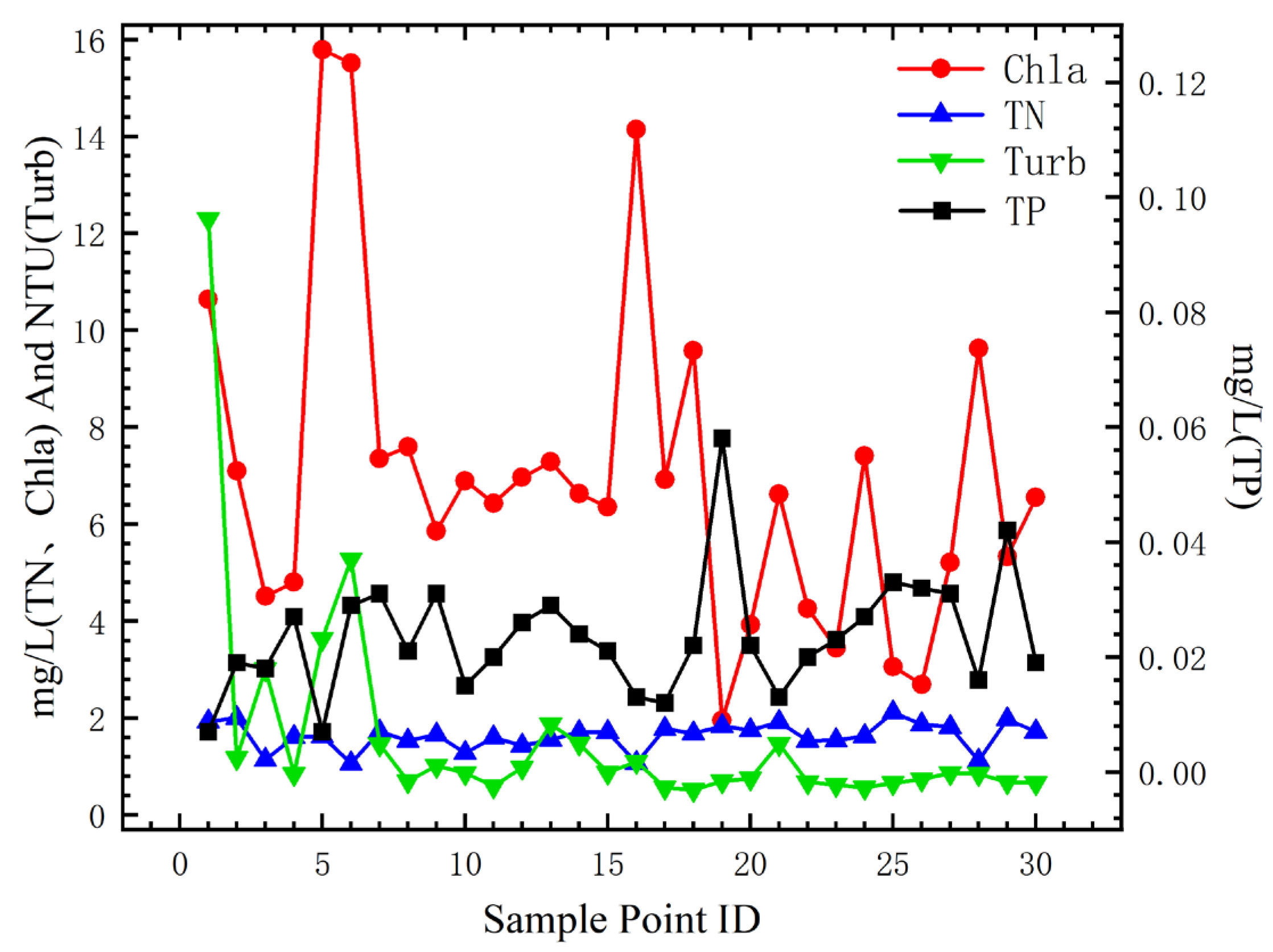
3.1. Pingzhai Reservoir Water Quality Information

Thirty water samples collected from Pingzhai Reservoir were analyzed, and their Chla, TN, TP, and Turb values are shown in Figure 2. It can be seen that the Chla values were located in the range of 1.95–15.79 mg/L, with a mean value of 7.013 mg/L. The TN values were located in the range of 1.063–2.120 mg/L, with a mean value of 1.729. The TP values were located in the range of 0.007–0.058 mg/L, with a mean value of 0.024 mg/L. The Turb values were located in the range of 0.515–12.3 NTU, with a mean value of 1.579 NTU.

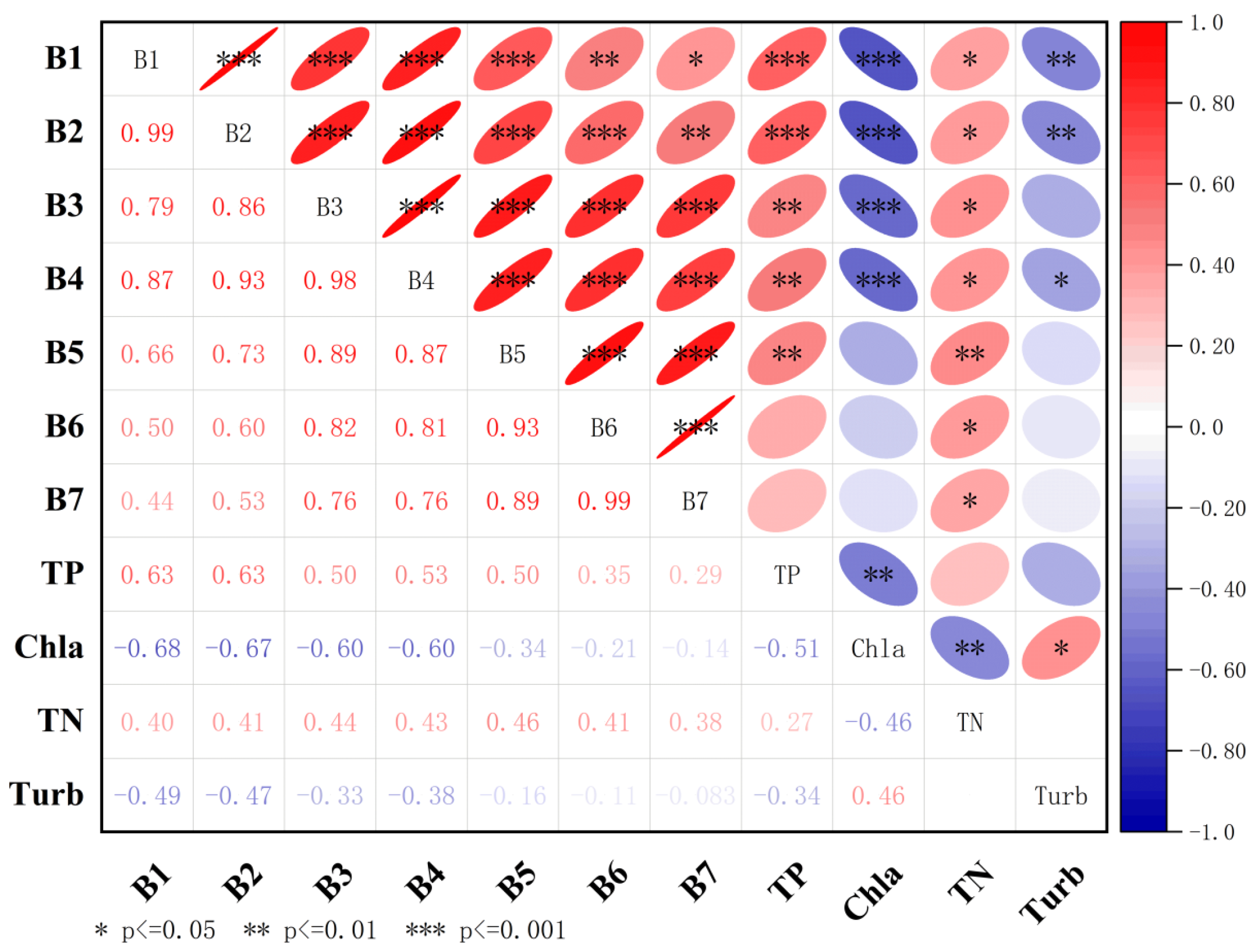
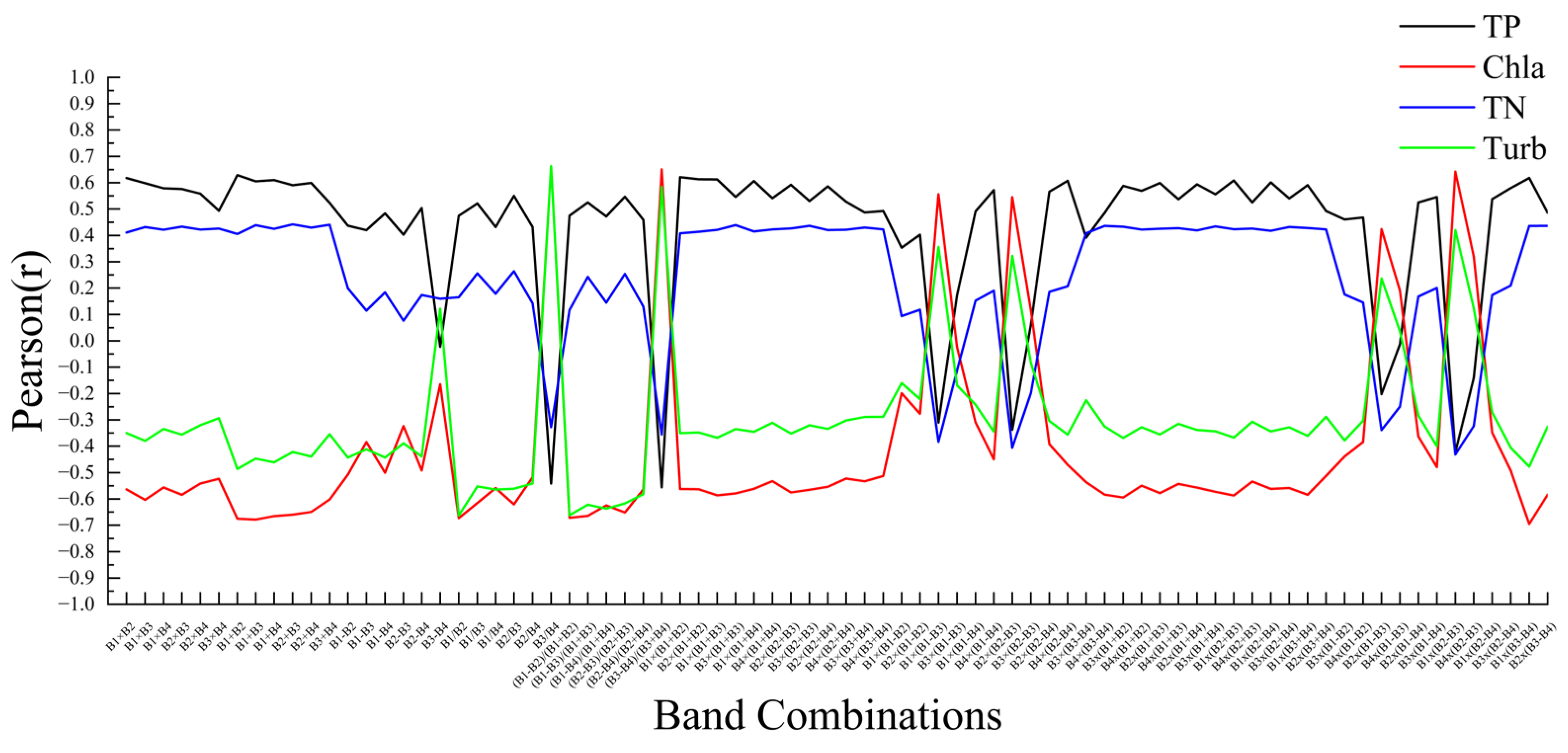
3.2. Correlation Analysis

For water quality inversion in inland water bodies, the visible to near-infrared (VNIR) bands are typically the most suitable spectral regions. Therefore, this study focused on analyzing B1–B7 bands of Landsat-8 OLI data. Using SPSS 26 statistical software, we examined the correlation between remotely sensed reflectance values and in situ measurements of Chla, TN, TP, and Turb at sampling locations. Pearson correlation coefficients were calculated to quantify these relationships, with results presented in Figure 3.
The analysis revealed significant correlations between water quality parameters and specific spectral bands. Chla showed strong negative correlations with B1 (r = −0.676), B2 (r = −0.670), and B3 (r = −0.598); TP exhibited positive correlations with B2 (r = 0.628), B1 (r = 0.627), and B4 (r = 0.538); TN demonstrated moderate positive correlations with B5 (r = 0.463), B3 (r = 0.442), and B4 (r = 0.432); and Turb displayed negative correlations with B1 (r = −0.494), B2 (r = −0.474), and B4 (r = −0.377).
To enhance these relationships, we evaluated various band combinations, including single-band, two-band, and three-band indices. As shown in Figure 4, band combinations generally improved correlation coefficients across all parameters. The most notable improvements were observed for Turb: B1/B2, B3/B4, and (B1−B2)/(B1+B2) (r = −0.663 for all); Chla: B1+B3 (r = −0.678) and B1/B2 (r = −0.673); TN: B2+B3 (r = 0.441); and TP: B1+B2 (r = 0.628);
These results demonstrate that carefully selected band combinations can enhance the correlation between spectral reflectance and water quality parameters compared to single-band analysis.

3.3. Multiple Regression Inversion Modeling

Multiple regression inversion modeling was performed by selecting three optimal spectral bands or band combinations exhibiting the strongest correlations with each water quality parameter. Using SPSS 26, we established multiple linear regression equations, with detailed results presented in Table 2. The modeling achieved higher accuracy for optically active parameters (Chla and Turb), whereas non-optically active parameters (TP and TN) showed relatively poor performance, consistent with their weaker spectral responses.

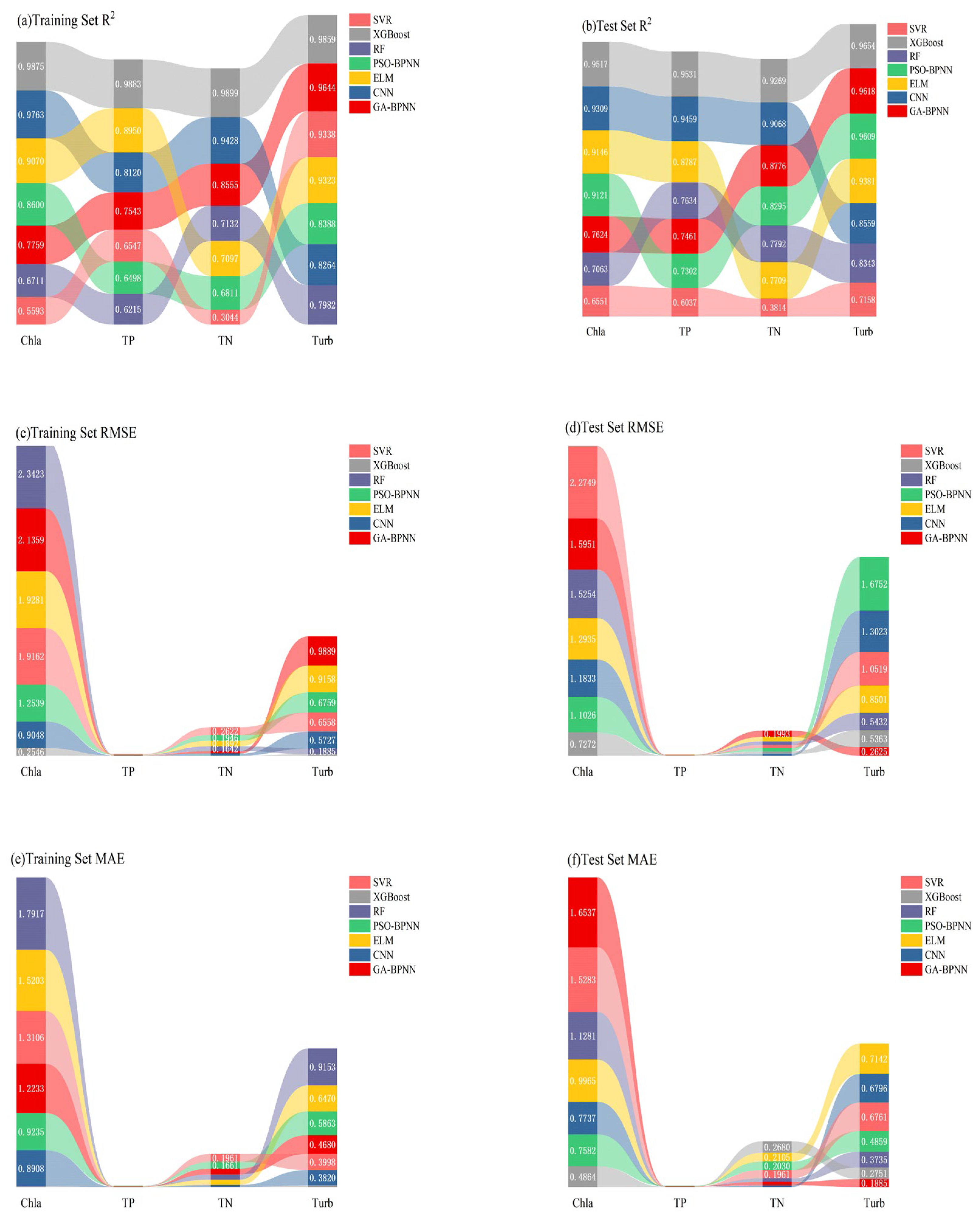
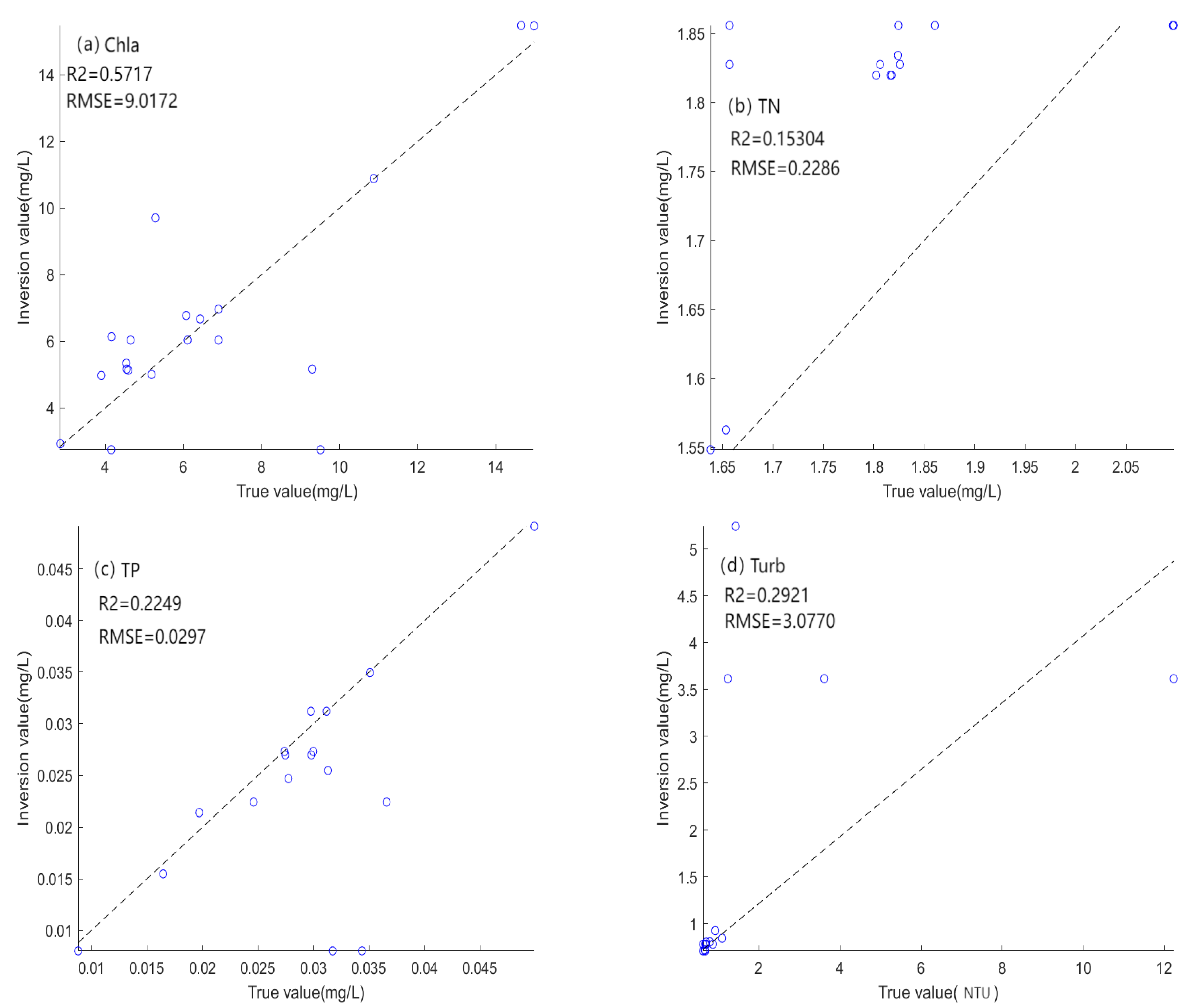
3.4. Machine Learning Inversion Model Construction

The 30 sampling points were divided into training and test sets at a 2:1 ratio, resulting in 20 samples for model training and 10 for validation. Using MATLAB R2020a, we developed machine learning models for four water quality parameters (Chla, TP, TN, and Turb) with seven algorithms: Support Vector Regression (SVR), Particle Swarm Optimization–Backpropagation Neural Network (PSO-BPNN), Genetic Algorithm–BPNN (GA-BPNN), Random Forest (RF), Convolutional Neural Network (CNN), Extreme Learning Machine (ELM), and XGBoost.
The results (Figure 5) demonstrate that the machine learning inversion models for the four water quality parameters are generally more accurate than the traditional regression models. Notably, the accuracy and stability of non-optically active parameters (TP and TN) improved significantly. This enhancement can be attributed to the complex, nonlinear relationships between these parameters and water reflectance, which machine learning algorithms can effectively capture, unlike linear regression methods.
Among all tested models, XGBoost exhibited the highest performance across all four water quality parameters while requiring the shortest training time compared to other algorithms. The inversion results were as follows: Chla: R2 = 0.9517, RMSE = 0.7272 mg/L, MAE = 0.4864 mg/L; TP: R2 = 0.9531, RMSE = 0.0017 mg/L, MAE = 0.0013 mg/L; TN: R2 = 0.9269, RMSE = 0.0793 mg/L, MAE = 0.0468 mg/L; Turb: R2 = 0.9654, RMSE = 0.5363 NTU, MAE = 0.2751 NTU. These findings highlight XGBoost’s superior capability in water quality parameter inversion, particularly for non-optically active constituents.

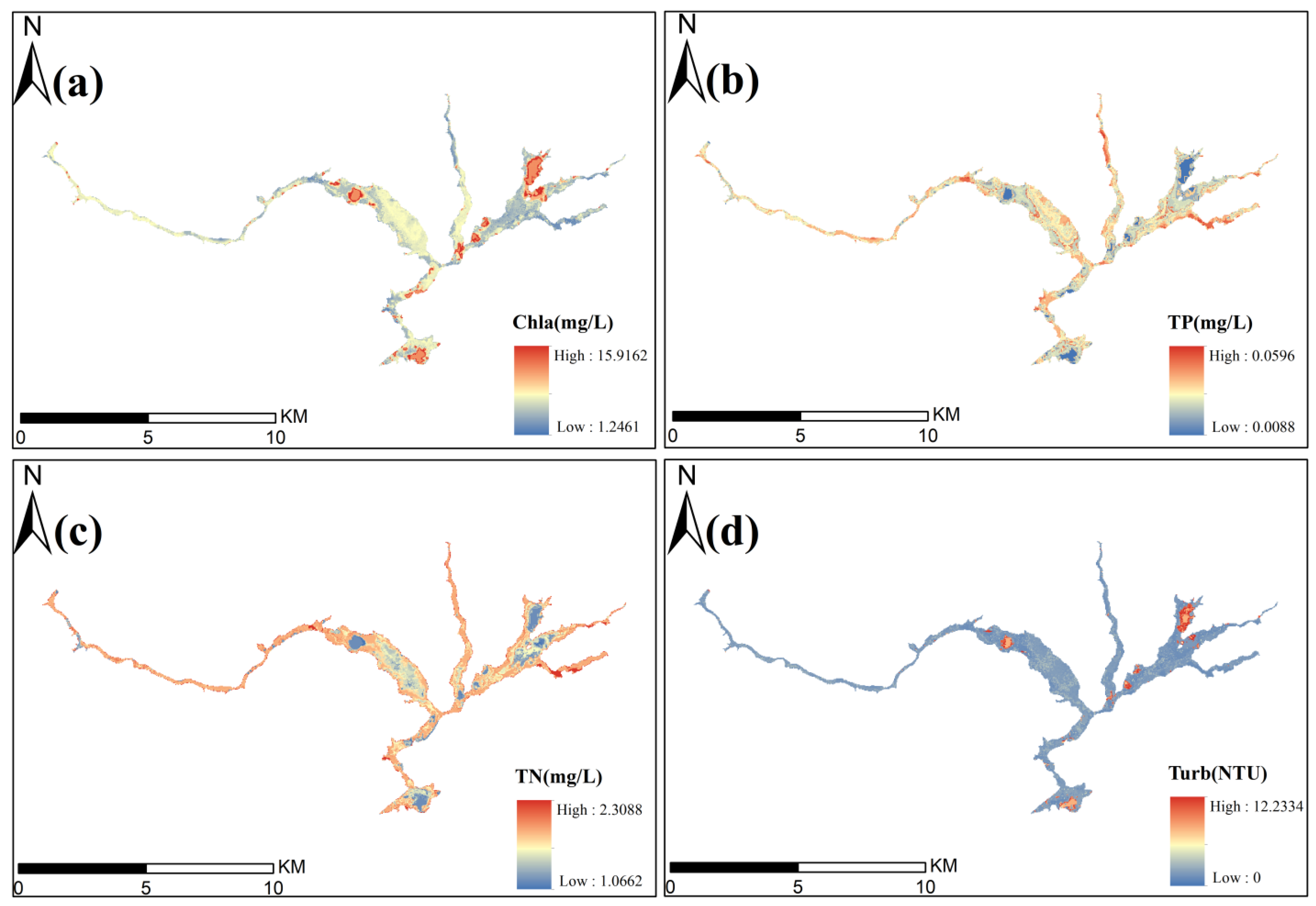
3.5. Spatial Distribution of WQIs in Pingzhai Reservoir

Using ArcGIS 10.8, the Pingzhai Reservoir area was delineated with a mask, and its reflectance values were extracted. The corresponding band combinations were then input into the trained XGBoost inversion model, yielding the spatial distribution results shown in Figure 6. The inversion results indicated the following concentration ranges: Chla at 1.2461–15.9162 mg/L, TP at 0.0088–0.0596 mg/L, TN at 1.0622–2.3088 mg/L, and Turb at 0–12.2334 NTU.
Spatially, higher Chla concentrations were observed in the northern Shuigong River, the southern reservoir area, and the open waters near the upper Nayong River. Interestingly, these regions exhibited lower TP and TN levels, while Turb increased alongside Chla. This spatial pattern aligns with the correlation analysis, which revealed a significant negative correlation between Chla and both TP and TN, as well as a strong positive correlation between Chla and Turb.

3.6. Analysis of the Applicability of the Model over Time

Designed specifically for karst plateau lakes, this study evaluates model performance under contrasting hydrological conditions. The July sampling (early wet season) captures complex optical water properties, allowing the training model to develop robustness against extreme conditions. Conversely, the May sampling (late dry season) represents relatively stable water quality parameters, providing an ideal scenario to test the model’s generalization capability under typical conditions. Therefore, to evaluate the model’s temporal applicability, field water samples were collected on 1 May 2024, and their physicochemical properties were analyzed using the same methodology. A Landsat-8 OLI satellite image (same orbit number as the previous dataset) was preprocessed identically, and the same spectral bands and band combinations were input into the pre-trained XGBoost inversion model for simulation. The results are presented in Figure 7.
The analysis revealed that the XGBoost model exhibited limited performance when applied to data from different time periods. The Chla inversion model achieved the highest accuracy, with an R2 of 0.5717 and an RMSE of 9.0172, while the TP inversion model performed the worst, yielding an R2 of 0.15304 and an RMSE of 0.2286. These results indicate that the model struggles to accurately predict water quality parameters across different temporal conditions.
In conclusion, models trained on single-period satellite imagery and in situ water quality data may have limited generalizability when applied to other time periods.

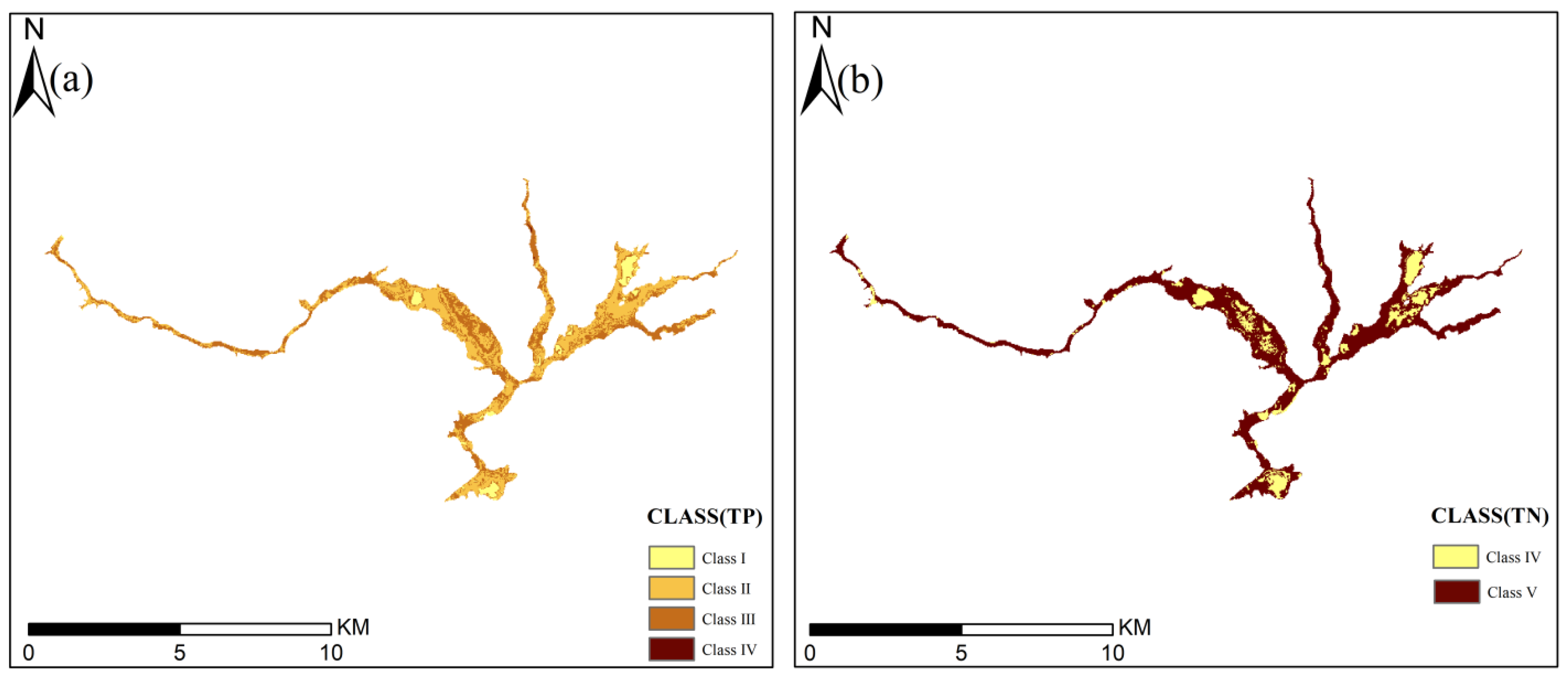
3.7. Water Quality Classification of Pingzhai Reservoir

According to the “People’s Republic of China Environmental Quality Standards for Surface Water” (GB 3838-2002), Environmental quality standards for surface water.The Ministry of Ecology and Environment: Beijing, China, 2002. the environmental quality of the lake and reservoir water was categorized into Classes I–V (as shown in Table 3), where Class I applies to source water and national nature reserves; Class II to centralized drinking water surface source primary protection zones, rare aquatic habitats, and fish spawning/feeding grounds; Class III to secondary drinking water protection zones, fishery wintering/migration areas, and swimming zones; Class IV to general industrial water and non-contact recreational use; and Class V to agricultural water and general landscape requirements.
Using the fitting results of the trained XGBoost model for classification (as shown in Figure 8), it can be found that with TN as the standard, the water quality of Pingzhai Reservoir is mainly class IV and V water, of which class IV water accounts for 19.60% of the total area, and class V water accounts for 80.40%. And to TP as a standard, Pingzhai Reservoir is mainly I–IV water, which accounts for, respectively, 5.97%, 52.07%, 41.83%, and 0.4%. More than 80% of the waters in Pingzhai Reservoir had TN content exceeding 2.0mg/L, which made it class V water, and thus TN became a more dominant pollutant compared to TP.

4. Discussion

4.1. Influence Between Chla, TN, TP, and Turb in Pingzhai Reservoir

According to the correlation analysis, Chla shows a significant negative correlation with TP and TN, and there is a weak positive correlation between TN and TP, while Turb has a poorer correlation with TP and TN but a more significant positive correlation with Chla. The same, more obvious trend as in the correlation analysis also appeared in the inversion results. In the northern part of the Shuigong River, the southern part of the reservoir area, and the upper part of the Nayong River open reservoir waters, there is a situation in which the values of Chla and Turb are larger, and TP and TN are smaller. Usually, TP and TN show positive correlation with Chla [40,47,48], while more studies have also appeared to show negative correlation of Chla with TN and TP [27,49]. Based on the reality of Pingzhai Reservoir, some scholars have proved that thermal stratification occurs in Pingzhai Reservoir during the summer period [50], and the thermocline refers to a transitional layer in a water body between the surface layer and the bottom layer, which is characterized by a sharp change in water temperature and density in this layer. This change is usually caused by seasonal changes in water temperature, with the surface layer being warmer in summer and the bottom layer being cooler due to lack of sunlight. The presence of a thermocline effectively hinders the exchange of material between the bottom and surface layers of the water column [51], so that Chla does not invade upwards in the form of bottom density currents. Excluding the influence of natural factors, the three areas with extreme values are all close to villages or towns and are in the area of open water. Therefore, the reason considered is that industrial and agricultural activities and wastewater discharge in villages and townships lead to large inputs of nutrients such as nitrogen and phosphorus, which result in eutrophication of the water bodies, and the growth of aquatic plants leads to higher Chla levels. Whereas the sampling date was located at the end of the summer season, which tends to have large sunshine hours, the light levels (7.00AM–7.00PM, Lux) for the week prior to the sampling date were obtained by using fully automated networked meteorological stations pre-buried in the different watersheds of the Pingzhai Reservoir (location shown in Figure 1), as shown in Table 4. It can be seen that, due to the altitude and weather and seasonal reasons, Pingzhai Reservoir area illuminance is larger, all located in more than 40,000 Lux. At the same time, the area where the extreme value appeared often has wider waters, resulting in a larger light surface, and the larger illuminance will exacerbate the photosynthesis of aquatic plants, and the increase in photosynthesis also increases the absorption of nutrients by aquatic plants [52]. Therefore, it also led to a more significant negative correlation between Chla and TP and TN. And some experiments proved that Chla showed a positive correlation with Turb in karst area [53].

4.2. Model Performance Analysis

Among the seven models tested, XGBoost demonstrated the best overall performance. Compared to the other six algorithms (GA-BPNN, CNN, ELM, PSO-BPNN, RF, and SVR), XGBoost improved the prediction accuracy for the test set by 14.64%, 4.50%, 8.92%, 11.77%, 23.57%, and 70.26%, respectively. This superior performance can be attributed to XGBoost’s iterative process of adding trees to fit the residuals of previous predictions, ultimately integrating these trees to enhance model accuracy. Additionally, the inclusion of a regularization term effectively mitigates overfitting, making XGBoost particularly suitable for modeling the complex, nonlinear relationships inherent in multi-factor-influenced water quality parameters.
In contrast, the SVR model exhibited the poorest performance, reducing the overall prediction accuracy for the test set by 16.38%, 42.10%, 39.62%, 39.24%, 7.81%, and 45.27% compared to the other six algorithms (GA-BPNN, CNN, ELM, PSO-BPNN, RF, and XGBoost), respectively. Notably, the SVR model achieved an R2 of only 0.3814 for the TN test set, indicating subpar performance. This may stem from SVR’s high sensitivity to parameter tuning and its limited ability to explore the entire sample space, potentially overlooking critical regions.
When applying the top-performing XGBoost model to fit measured data from Pingzhai Reservoir across different periods, the overall predictive performance was unsatisfactory (R2 < 0.6). The Chla inversion model yielded the best results, with an R2 of 0.5717 and an RMSE of 9.017 mg/L, while the TN inversion model performed worst, with an R2 of 0.15304 and an RMSE of 0.2286. These findings suggest that water quality parameters exhibit significant variability across different periods, making it challenging to predict parameters for other periods using models trained on single-period data.

4.3. Limitations and Perspectives

The inversion model established in this paper still has some limitations, and the discrepancy between the model-predicted value and the measured value still exists, which may be caused by the influence of several factors. Firstly, the spatial resolution of the remote sensing image used in this paper is relatively low (30 m), which may be affected by other interfering factors in a single pixel, thus decreasing the accuracy. The output parameter of the model is the average water quality parameter value within a single image element, which may not correspond to the water quality parameter value of the established sampling sites. Secondly, in karst plateau mountainous regions, frequent cloud cover poses the greatest challenge for acquiring valid satellite remote sensing imagery. Particularly in lake and reservoir areas, persistent cloud interference makes it difficult to obtain effective water surface information through remote sensing, thereby hindering fixed time-series studies. This limitation further explains why Sentinel-2 MSI satellite imagery could not be effectively utilized in this study. While Sentinel-2 offers superior spatiotemporal resolution in theory, all available scenes during the 15 days above and below the sampling time exhibited >80% cloud cover over Pingzhai Reservoir, rendering water surface data extraction unfeasible. In contrast, Landsat 8 provided two usable scenes with <15% cloud coverage, allowing for reliable acquisition of water surface information.
When establishing surface sampling points, accurately characterizing the average value of a single pixel in lower spatial resolution imagery remains challenging. To enhance input layer interpretability, a practical solution involves deploying multiple sampling points within a single pixel and using their averaged measurements. Additionally, for acquiring effective satellite remote sensing data in karst mountainous regions, low-altitude remote sensing platforms (UAVs) offer significant advantages. UAV remote sensing not only provides higher spatial and spectral resolution imagery but also enables flexible temporal sampling. However, implementation challenges persist due to the dramatic terrain undulations and fragmented land parcels characteristic of karst landscapes [54].This study employs seven conventional machine learning algorithms for comparative model development. As machine learning techniques continue to advance, future research should explore more sophisticated algorithms specifically optimized for water quality parameter inversion from remote sensing data, thereby contributing more robust scientific methodologies to the field.

5. Conclusions

In summary, the Landsat-8 OLI satellite remote sensing image data and the measured data of field water samples were analyzed using seven different machine algorithms (GA-BPNN, CNN, ELM, PSO-BPNN, RF, XGBoost, and SVR) and multiple linear regression analysis, and their inverse models were established for each of the four water quality parameters (Chla, TP, TN, and Turb). Models and their performances were compared by three evaluation indexes, namely, R2, RMSE, and MAE. In total, the following conclusions were drawn: (1) By correlation analysis, the Landsat-8 OLI bands with the strongest correlations with Chla were B2, (B1/B2), and (B1+B3); the strongest correlations with TP were B1, B2, and (B1+B2); the strongest correlations with TN were B5, (B2+B3), and B3; and the strongest correlations with Turb were (B1/B2), (B3/B4), and (B1−B2)/(B1+B2). (2) Through the multivariate linear modeling, the optically active water quality parameters Chla and Turb have better results, while the non-optically active water quality parameters TP and TN have poorer results. (3) Through the establishment of machine learning models, the performance of machine models is greater than that of the traditional multivariate linear models, and the improvement is greater for the non-optically active water quality parameters TP and TN. The best performance is the XGBoost inversion model, which has a fitting R2 greater than 0.9 for all four water quality parameters in the test set; the worst performance is the SVR model. (4) At the end of summer in the Karst Plateau/Pingzhai Reservoir, the wider watershed area showed a more significant negative correlation between Chla and TN and TP due to the strong illumination. (5) Inversion models trained using single-period imagery are poorly fitted to the same areas in different periods, and the use of a single model to predict water quality parameters in different periods is still somewhat limited.

Author Contributions

Data curation, C.W., Y.W., L.L., C.D., R.L. and X.Z.; funding acquisition, Z.Z.; investigation, J.K.; methodology, R.X.; project administration, R.X.; resources, Z.Z.; software, R.X.; validation, C.W.; visualization, R.X.; writing—original draft, R.X.; writing—review and editing, R.X. and J.K. All authors have read and agreed to the published version of the manuscript.

Funding

This study was supported financially by the National Natural Science Foundation of China (42161048) and the National Natural Science Foundation of China (41661088).

Data Availability Statement

The datasets generated during and/or analyzed during the current study are available from the corresponding author upon reasonable request.

Acknowledgments

Thanks to USGS for providing the Landsat-8 images.

Conflicts of Interest

The authors declare no conflicts of interest.

References

  1. Li, T.; Qiu, S.; Mao, S.X.; Bao, R.; Deng, H.B. Evaluating Water Resource Accessibility in Southwest China. Water 2019, 11, 1708. [Google Scholar] [CrossRef]
  2. Wang, M.R.; Bodirsky, B.L.; Rijneveld, R.; Beier, F.; Bak, M.P.; Batool, M.; Droppers, B.; Popp, A.; van Vliet, M.T.H.; Strokal, M. A triple increase in global river basins with water scarcity due to future pollution. Nat. Commun. 2024, 15, 880. [Google Scholar] [CrossRef] [PubMed]
  3. Ellis, E.A.; Allen, G.H.; Riggs, R.M.; Gao, H.L.; Li, Y.; Carey, C.C. Bridging the divide between inland water quantity and quality with satellite remote sensing: An interdisciplinary review. Wiley Interdiscip. Rev. Water 2024, 11, e1725. [Google Scholar] [CrossRef]
  4. Dong, L.; Gong, C.L.; Wang, X.H.; Wang, Y.; He, D.G.; Hu, Y.; Li, L.; Yang, Z. Seasonal Monitoring Method for TN and TP Based on Airborne Hyperspectral Remote Sensing Images. Remote Sens. 2024, 16, 1614. [Google Scholar] [CrossRef]
  5. Wang, S.Y.; Shen, M.; Liu, W.H.; Ma, Y.X.; Shi, H.; Zhang, J.T.; Liu, D. Developing remote sensing methods for monitoring water quality of alpine rivers on the Tibetan Plateau. Gisci. Remote Sens. 2022, 59, 1384–1405. [Google Scholar] [CrossRef]
  6. Mohsen, A.; Elshemy, M.; Zeidan, B. Water quality monitoring of Lake Burullus (Egypt) using Landsat satellite imageries. Environ. Sci. Pollut. Res. 2021, 28, 15687–15700. [Google Scholar] [CrossRef]
  7. Chen, P.; Wang, B.; Wu, Y.L.; Wang, Q.J.; Huang, Z.J.; Wang, C.L. Urban river water quality monitoring based on self-optimizing machine learning method using multi-source remote sensing data. Ecol. Indic. 2023, 146, 109750. [Google Scholar] [CrossRef]
  8. Tian, S.; Guo, H.W.; Xu, W.; Zhu, X.T.; Wang, B.; Zeng, Q.H.; Mai, Y.Q.; Huang, J.H.J. Remote sensing retrieval of inland water quality parameters using Sentinel-2 and multiple machine learning algorithms. Environ. Sci. Pollut. Res. 2023, 30, 18617–18630. [Google Scholar] [CrossRef]
  9. Wei, L.F.; Wang, Z.; Huang, C.; Zhang, Y.; Wang, Z.X.; Xia, H.Q.; Cao, L.Q. Transparency Estimation of Narrow Rivers by UAV-Borne Hyperspectral Remote Sensing Imagery. IEEE Access 2020, 8, 168137–168153. [Google Scholar] [CrossRef]
  10. Cruz-Retana, A.; Becerril-Piña, R.; Fonseca, C.R.; Gomez-Albores, M.A.; Gaytan-Aguilar, S.; Hernández-Téllez, M.; Mastachi-Loza, C.A. Assessment of Regression Models for Surface Water Quality Modeling via Remote Sensing of a Water Body in the Mexican Highlands. Water 2023, 15, 3828. [Google Scholar] [CrossRef]
  11. Peng, C.C.; Xie, Z.J.; Jin, X. Using Ensemble Learning for Remote Sensing Inversion of Water Quality Parameters in Poyang Lake. Sustainability 2024, 16, 3355. [Google Scholar] [CrossRef]
  12. Yépez, S.; Velásquez, G.; Torres, D.; Saavedra-Passache, R.; Pincheira, M.; Cid, H.; Rodríguez-López, L.; Contreras, A.; Frappart, F.; Cristóbal, J.; et al. Spatiotemporal Variations in Biophysical Water Quality Parameters: An Integrated In Situ and Remote Sensing Analysis of an Urban Lake in Chile. Remote Sens. 2024, 16, 427. [Google Scholar] [CrossRef]
  13. Liu, B.; Li, T.H. A Machine-Learning-Based Framework for Retrieving Water Quality Parameters in Urban Rivers Using UAV Hyperspectral Images. Remote Sens. 2024, 16, 905. [Google Scholar] [CrossRef]
  14. Fu, B.L.; Lao, Z.A.; Liang, Y.Y.; Sun, J.; He, X.; Deng, T.F.; He, W.; Fan, D.L.; Gao, E.R.; Hou, Q.L. Evaluating optically and non-optically active water quality and its response relationship to hydro-meteorology using multi-source data in Poyang Lake, China. Ecol. Indic. 2022, 145, 109675. [Google Scholar] [CrossRef]
  15. Wang, C.L.; Shi, K.Y.; Ming, X.; Cong, M.Q.; Liu, X.Y.; Guo, W.J. A Comparative Study of the COD Hyperspectral Inversion Models in Water Based on the Maching Learning. Spectrosc. Spectr. Anal. 2022, 42, 2353–2358. [Google Scholar] [CrossRef]
  16. Wu, D.; Jiang, J.; Wang, F.Y.; Luo, Y.R.; Lei, X.D.; Lai, C.G.; Wu, X.S.; Xu, M.H. Retrieving Eutrophic Water in Highly Urbanized Area Coupling UAV Multispectral Data and Machine Learning Algorithms. Water 2023, 15, 354. [Google Scholar] [CrossRef]
  17. Sagan, V.; Peterson, K.T.; Maimaitijiang, M.; Sidike, P.; Sloan, J.; Greeling, B.A.; Maalouf, S.; Adams, C. Monitoring inland water quality using remote sensing: Potential and limitations of spectral indices, bio-optical simulations, machine learning, and cloud computing. Earth-Sci. Rev. 2020, 205, 103187. [Google Scholar] [CrossRef]
  18. Guo, H.W.; Huang, J.J.; Zhu, X.T.; Tian, S.; Wang, B.L. Spatiotemporal variation reconstruction of total phosphorus in the Great Lakes since 2002 using remote sensing and deep neural network. Water Res. 2024, 255, 121493. [Google Scholar] [CrossRef]
  19. Zhou, Y.D.; Li, W.; Cao, X.Y.; He, B.Y.; Feng, Q.; Yang, F.; Liu, H.; Kutser, T.; Xu, M.; Xiao, F.; et al. Spatial-temporal distribution of labeled set bias remote sensing estimation: An implication for supervised machine learning in water quality monitoring. Int. J. Appl. Earth Obs. Geoinf. 2024, 131, 103959. [Google Scholar] [CrossRef]
  20. Tang, X.D.; Huang, M.T. Inversion of Chlorophyll-a Concentration in Donghu Lake Based on Machine Learning Algorithm. Water 2021, 13, 1179. [Google Scholar] [CrossRef]
  21. He, Y.H.; Gong, Z.J.; Zheng, Y.H.; Zhang, Y.B. Inland Reservoir Water Quality Inversion and Eutrophication Evaluation Using BP Neural Network and Remote Sensing Imagery: A Case Study of Dashahe Reservoir. Water 2021, 13, 2844. [Google Scholar] [CrossRef]
  22. Ren, J.H.; Cui, J.Y.; Dong, W.; Xiao, Y.F.; Xu, M.M.; Liu, S.W.; Wan, J.H.; Li, Z.W.; Zhang, J. Remote Sensing Inversion of Typical Offshore Water Quality Parameter Concentration Based on Improved SVR Algorithm. Remote Sens. 2023, 15, 2104. [Google Scholar] [CrossRef]
  23. Guo, Q.Z.; Wu, H.H.; Jin, H.Y.; Yang, G.; Wu, X.X. Remote Sensing Inversion of Suspended Matter Concentration Using a Neural Network Model Optimized by the Partial Least Squares and Particle Swarm Optimization Algorithms. Sustainability 2022, 14, 2221. [Google Scholar] [CrossRef]
  24. Wang, L.; Wang, X.; Zhou, C.; Wang, X.X.; Meng, Q.H.; Chen, Y.L. Remote Sensing Quantitative Retrieval of Chlorophyll a and Trophic Level Index in Main Seagoing Rivers of Lianyungang. Spectrosc. Spectr. Anal. 2023, 43, 3314–3320. [Google Scholar]
  25. Ai, B.; Wen, Z.; Jiang, Y.C.; Gao, S.; Lv, G.N. Sea surface temperature inversion model for infrared remote sensing images based on deep neural network. Infrared Phys. Technol. 2019, 99, 231–239. [Google Scholar] [CrossRef]
  26. Dai, J.J.; Liu, T.Y.; Zhao, Y.Y.; Tian, S.F.; Ye, C.Y.; Nie, Z. Remote sensing inversion of the Zabuye Salt Lake in Tibet, China using LightGBM algorithm. Front. Earth Sci. 2023, 10, 1022280. [Google Scholar] [CrossRef]
  27. Li, Y.L.; Zhou, Z.F.; Kong, J.; Wen, C.C.; Li, S.H.; Zhang, Y.R.; Xie, J.T.; Wang, C. Monitoring Chlorophyll-a concentration in karst plateau lakes using Sentinel 2 imagery from a case study of pingzhai reservoir in Guizhou, China. Eur. J. Remote Sens. 2022, 55, 1–19. [Google Scholar] [CrossRef]
  28. Chun, H. Reservoir Capacity Calculation of Karst Underground Reservoir Associated with Pingzhai Reservoir in Deep Canyon Area of Upper Reaches of Wujiang River. Resour. Environ. Eng. 2021, 35, 478–483. [Google Scholar]
  29. Renau-Pruñonosa, A.; Morell, I.; Pulido-Velazquez, D. A Methodology to Analyse and Assess Pumping Management Strategies in Coastal Aquifers to Avoid Degradation Due to Seawater Intrusion Problems. Water Resour. Manag. 2016, 30, 4823–4837. [Google Scholar] [CrossRef]
  30. Zhang, Y.R.; Zhou, Z.F.; Zhang, H.T.; Dan, Y.S. Quantifying the impact of human activities on water quality based on spatialization of social data: A case study of the Pingzhai Reservoir Basin. Water Supply 2020, 20, 688–699. [Google Scholar] [CrossRef]
  31. Jain, S.; Rastogi, R. Parametric non-parallel support vector machines for pattern classification. Mach. Learn. 2024, 113, 1567–1594. [Google Scholar] [CrossRef]
  32. Sun, L.; Bao, J.; Chen, Y.Y.; Yang, M.M. Research on parameter selection method for support vector machines. Appl. Intell. 2018, 48, 331–342. [Google Scholar] [CrossRef]
  33. Yang, A.M.; Zhuansun, Y.X.; Liu, C.S.; Li, J.; Zhang, C.Y. Design of Intrusion Detection System for Internet of Things Based on Improved BP Neural Network. IEEE Access 2019, 7, 106043–106052. [Google Scholar] [CrossRef]
  34. Zhu, W.D.; Kong, Y.X.; He, N.Y.; Qiu, Z.G.; Lu, Z.G. Prediction and Analysis of Chlorophyll-a Concentration in the Western Waters of Hong Kong Based on BP Neural Network. Sustainability 2023, 15, 10441. [Google Scholar] [CrossRef]
  35. Hu, H.; Fu, X.L.; Li, H.H.; Wang, F.; Duan, W.J.; Zhang, L.Q.; Liu, M. Prediction of lake chlorophyll concentration using the BP neural network and Sentinel-2 images based on time features. Water Sci. Technol. 2023, 87, 539–554. [Google Scholar] [CrossRef]
  36. Xiao, X.; Song, B.Y.; Wen, X.F.; Zhao, D.Z.; Cheng, X.J.; Hu, C.F.; Xu, J.; Wang, Z.H. VIP-BP model for retrieving chlorophyll a concentration in the river by using remote sensing data. Water Qual. Res. J. Can. 2017, 52, 136–150. [Google Scholar] [CrossRef]
  37. Zhao, W.J.; Ma, H.; Zhou, C.; Zhou, C.Q.; Li, Z.L. Soil Salinity Inversion Model Based on BPNN Optimization Algorithm for UAV Multispectral Remote Sensing. IEEE J. Sel. Top. Appl. Earth Obs. Remote Sens. 2023, 16, 6038–6047. [Google Scholar] [CrossRef]
  38. Li, J.M.; Dong, X.; Ruan, S.M.; Shi, L. A parallel integrated learning technique of improved particle swarm optimization and BP neural network and its application. Sci. Rep. 2022, 12, 19325. [Google Scholar] [CrossRef]
  39. Mantas, C.J.; Castellano, J.G.; Moral-García, S.; Abellán, J. A comparison of random forest based algorithms: Random credal random forest versus oblique random forest. Soft Comput. 2019, 23, 10739–10754. [Google Scholar] [CrossRef]
  40. Song, W.; Yinglan, A.; Wang, Y.T.; Fang, Q.Q.; Tang, R. Study on remote sensing inversion and temporal-spatial variation of Hulun lake water quality based on machine learning. J. Contam. Hydrol. 2024, 260, 104282. [Google Scholar] [CrossRef]
  41. Lo, Y.; Fu, L.; Lu, T.C.; Huang, H.; Kong, L.R.; Xu, Y.Q.; Zhang, C. Medium-Sized Lake Water Quality Parameters Retrieval Using Multispectral UAV Image and Machine Learning Algorithms: A Case Study of the Yuandang Lake, China. Drones 2023, 7, 244. [Google Scholar] [CrossRef]
  42. Li, Z.H.; Chen, C.; Cao, N.X.; Jiang, Z.H.; Liu, C.J.; Oke, S.A.; Jim, C.; Zheng, K.X.; Zhang, F. High spatial resolution inversion of chromophoric dissolved organic matter (CDOM) concentrations in Ebinur Lake of arid Xinjiang, China: Implications for surface water quality monitoring. Int. J. Appl. Earth Obs. Geoinf. 2024, 132, 104022. [Google Scholar] [CrossRef]
  43. Xue, Y.; Zhu, L.; Zou, B.; Wen, Y.M.; Long, Y.H.; Zhou, S.L. Research on Inversion Mechanism of Chlorophyll-A Concentration in Water Bodies Using a Convolutional Neural Network Model. Water 2021, 13, 664. [Google Scholar] [CrossRef]
  44. Zhou, Z.Y.; Chen, J.; Zhu, Z.F. Regularization incremental extreme learning machine with random reduced kernel for regression. Neurocomputing 2018, 321, 72–81. [Google Scholar] [CrossRef]
  45. Zhang, Y.B.; Shi, K.; Sun, X.; Zhang, Y.L.; Li, N.; Wang, W.J.; Zhou, Y.Q.; Zhi, W.; Liu, M.L.; Li, Y.; et al. Improving remote sensing estimation of Secchi disk depth for global lakes and reservoirs using machine learning methods. Gisci. Remote Sens. 2022, 59, 1367–1383. [Google Scholar] [CrossRef]
  46. Sun, Z.H.; Guo, L.; Tao, Z.; Li, Y.A.; Zhan, Y.; Li, S.L.; Zhao, Y. Water Quality Inversion Framework for Taihu Lake Based on Multilayer Denoising Autoencoder and Ensemble Learning. Remote Sens. 2024, 16, 4793. [Google Scholar] [CrossRef]
  47. Chen, B.T.; Mu, X.; Chen, P.; Wang, B.A.; Choi, J.; Park, H.; Xu, S.; Wu, Y.L.; Yang, H. Machine learning-based inversion of water quality parameters in typical reach of the urban river by UAV multispectral data. Ecol. Indic. 2021, 133, 108434. [Google Scholar] [CrossRef]
  48. Wu, B.W.; Dai, S.N.; Wen, X.L.; Qian, C.; Luo, F.; Xu, J.Q.; Wang, X.D.; Li, Y.; Xi, Y.L. Chlorophyll-nutrient relationship changes with lake type, season and small-bodied zooplankton in a set of subtropical shallow lakes. Ecol. Indic. 2022, 135, 108571. [Google Scholar] [CrossRef]
  49. Guo, Z.; Li, C.Y.; Shi, X.H.; Sun, B. Spatial and Temporal Distribution Characteristics of Chlorophyll A Contentand lts Influencing Factor Analysis in Hulun Lake of Cold and Dry Areas. Ecol. Environ. Sci. 2019, 28, 1434–1442. [Google Scholar]
  50. Liu, X. Changes of Hydrochemistry and Dissolved lnorganic Carbon DurincThermal Stratification in Pingzhai Reservoir. Resour. Environ. Yangtze Basin 2021, 30, 936–945. [Google Scholar]
  51. Chowdhury, M.S.A.; Hasan, K.; Alam, K. The Use of an Aeration System to Prevent Thermal Stratification of Water Bodies: Pond, Lake and Water Supply Reservoir. Appl. Ecol. Environ. Sci. 2014, 2, 1–7. [Google Scholar] [CrossRef]
  52. Wang, Z.H.; Wang, C.Z.; Wang, X.; Wang, B.; Wu, J.; Liu, L.L. Aerosol pollution alters the diurnal dynamics of sun and shade leaf photosynthesis through different mechanisms. Plant Cell Environ. 2022, 45, 2943–2953. [Google Scholar] [CrossRef] [PubMed]
  53. Yang, W.L.; Fu, B.L.; Li, S.Z.; Lao, Z.N.; Deng, T.F.; He, W.; He, H.C.; Chen, Z.K. Monitoring multi-water quality of internationally important karst wetland through deep learning, multi-sensor and multi-platform remote sensing images: A case study of Guilin, China. Ecol. Indic. 2023, 154, 110755. [Google Scholar] [CrossRef]
  54. Huang, D. Challenges and main research advances of low-altitude remote sensing forcrops in southwest plateau mountains. J. Guizhou Norm. Univ. Nat. Sci. 2021, 39, 51–59. [Google Scholar]
Figure 1. Location of the Pingzhai Reservoir.
Water 17 01781 g001
Figure 2. Water quality objectives of Pingzhai Reservoir.
Water 17 01781 g002
Figure 3. Pearson correlation coefficient between water quality parameters and single bands.
Water 17 01781 g003
Figure 4. Pearson correlation coefficient of water quality parameters and bands combined.
Water 17 01781 g004
Figure 5. Comparison of the accuracy of different machine models. (a) Training Set R2; (b) Test Set R2; (c) Training Set RMSE; (d) Test Set RMSE; (e) Training Set MAE; and (f) Test Set MAE.
Water 17 01781 g005
Figure 6. Distribution of the four WQIs. (a) Chla; (b) TP; (c) TN; and (d) Turb.
Water 17 01781 g006
Figure 7. The fitting results of the XGBoost model for four WQIs in different periods. (a) Chla; (b) TN; (c) TP; and (d) Turb.
Water 17 01781 g007
Figure 8. Water classes for different indicators. (a) TP; (b) TN.
Water 17 01781 g008
Table 1. Landsat-8 band parameters.
SensorBand NameBandwidth (μm)Resolution (m)
Operational Land Imager (OLI)Band 1 Coastal0.43–0.4530
Band 2 Blue0.45–0.5130
Band 3 Green0.53–0.5930
Band 4 Red0.64–0.6730
Band 5 NIR0.85–0.8830
Band 6 SWIR 11.57–1.6530
Band 7 SWIR 22.11–2.2930
Band 8 Pan0.50–0.6815
Band 9 Cirrus1.36–1.3830
Thermal Infrared Sensor (TIRS)Band 10 TIRS 110.6–11.19100
Band 11 TIRS 211.5–12.51100
Table 2. Multiple regression model establishment results.
WQIsModelR2RMSEMAE
ChlaChla = 900.418 × B1 − 12.812 × B1/B2 − 516.495 × (B1 + B3) + 29.4040.6532.12091.5385
TPTP = 0.131 × B2 + 0.266 × (B1 + B2) + 0.0090.3960.00830.0057
TNTN = 8.964 × B5 + 5.083 × (B2 + B3) − 5.908 × B3 + 1.3810.2770.22510.1840
TurbTurb = 2.671 × (B3/B4) − 3.731 × (B1/B2) − 2.073 [(B1 − B2)/(B1 + B2)] + 0.0490.5521.50641.0757
Table 3. Water classification standards.
Class
TN <= (mg/L)0.20.51.01.52.0
TP <= (mg/L)0.010.0250.050.10.2
Table 4. Light intensity one week prior to sampling (Lux).
7/217/227/237/247/257/267/27
WS135,175.4461,735.5561,886.8963,728.3369,642.7971,569.7542,283.63
WS247,498.5567,062.0658,931.3664,571.7269,273.4069,832.7847,005.43
WS341,796.6164,079.0269,123.2768,803.6768,653.3777,863.4149,377.34
AVR41,490.064,292.2163,313.8465,701.2469,189.8573,088.6546,222.13
Disclaimer/Publisher’s Note: The statements, opinions and data contained in all publications are solely those of the individual author(s) and contributor(s) and not of MDPI and/or the editor(s). MDPI and/or the editor(s) disclaim responsibility for any injury to people or property resulting from any ideas, methods, instructions or products referred to in the content.

