Abstract
High-quality precipitation data are vital for hydrological research. In regions with sparse observation stations, reliable gridded data cannot be obtained through interpolation, while the coarse resolution of satellite products fails to meet the demands of small watershed studies. Downscaling satellite-based precipitation products offers an effective solution for generating high-resolution data in such areas. Among these techniques, machine learning plays a pivotal role, with performance varying according to surface conditions and algorithmic mechanisms. Using the Qinghai Lake Basin as a case study and rain gauge observations as reference data, this research conducted a systematic comparative evaluation of nine machine learning algorithms (ANN, CLSTM, GAN, KNN, MSRLapN, RF, SVM, Transformer, and XGBoost) for downscaling IMERG precipitation products from 0.1° to 0.01° resolution. The primary objective was to identify the optimal downscaling method for the Qinghai Lake Basin by assessing spatial accuracy, seasonal performance, and residual sensitivity. Seven metrics were employed for assessment: correlation coefficient (CC), root mean square error (RMSE), mean absolute error (MAE), coefficient of determination (R2), standard deviation ratio (Sigma Ratio), Kling-Gupta Efficiency (KGE), and bias. On the annual scale, KNN delivered the best overall results (KGE = 0.70, RMSE = 17.09 mm, Bias = −3.31 mm), followed by Transformer (KGE = 0.69, RMSE = 17.20 mm, Bias = −3.24 mm). During the cold season, KNN and ANN both performed well (KGE = 0.63; RMSE = 5.97 mm and 6.09 mm; Bias = −1.76 mm and −1.75 mm), with SVM ranking next (KGE = 0.63, RMSE = 6.11 mm, Bias = −1.63 mm). In the warm season, Transformer yielded the best results (KGE = 0.74, RMSE = 23.35 mm, Bias = −1.03 mm), followed closely by ANN and KNN (KGE = 0.74; RMSE = 23.38 mm and 23.57 mm; Bias = −1.08 mm and −1.03 mm, respectively). GAN consistently underperformed across all temporal scales, with annual, cold-season, and warm-season KGE values of 0.61, 0.43, and 0.68, respectively—worse than the original 0.1° IMERG product. Considering the ability to represent spatial precipitation gradients, KNN emerged as the most suitable method for IMERG downscaling in the Qinghai Lake Basin. Residual analysis revealed error concentrations along the lakeshore, and model performance declined when residuals exceeded specific thresholds—highlighting the need to account for model-specific sensitivity during correction. SHAP analysis based on ANN, KNN, SVM, and Transformer identified NDVI (0.218), longitude (0.214), and latitude (0.208) as the three most influential predictors. While longitude and latitude affect vapor transport by representing land–sea positioning, NDVI is heavily influenced by anthropogenic activities and sandy surfaces in lakeshore regions, thus limiting prediction accuracy in these areas. This work delivers a high-resolution (0.01°) precipitation dataset for the Qinghai Lake Basin and provides a practical basis for selecting suitable downscaling methods in similar environments.
1. Introduction
As a fundamental element of the hydrological cycle [1], precipitation exerts a profound influence on ecosystems [2], regulates surface energy exchanges [3], and shapes human-environment interactions [4]. Accurate quantification of both the magnitude and spatial distribution of precipitation is indispensable for a wide range of applications, including regional water resource management [5], hydrological modeling, and climate attribution studies [6]. Furthermore, its spatiotemporal variability offers key insights into the mechanisms driving global climate change [7]. Nevertheless, in regions characterized by complex and heterogeneous terrain, acquiring high-resolution and reliable precipitation data remains a persistent and formidable challenge [8].
While point-based precipitation measurements from rain gauges offer high temporal resolution [9], they lack the spatial representativeness needed for capturing fine-scale variability [10]. Conversely, satellite-derived precipitation products provide extensive spatial coverage [11], and their inherent coarse resolutions (e.g., 0.25° × 0.25° or 0.1° × 0.1°) lead to significant smoothing of precipitation gradients in small watersheds. This resolution limitation substantially constrains their effectiveness for critical watershed management applications, including water resources optimization, accurate identification of precipitation events [12], and timely disaster monitoring [13].
This limitation underscores the necessity of spatial downscaling to enhance the applicability of satellite products in fine-scale hydrological modeling. Downscaling techniques are broadly classified into dynamical and statistical approaches [14]. Dynamical downscaling relies heavily on Regional Climate Models (RCMs), which employ rigorous mathematical and physical foundations to simulate land-atmosphere coupling processes for obtaining high-resolution climatic factors [15]. This high-resolution precipitation data assimilation (DA) technique has been successfully applied in weather forecasting models [16], with common assimilation algorithms including Three-Dimensional Variational (3D-Var) [17] and Four-Dimensional Variational (4D-Var) [18]. However, this approach demands substantial computational resources as resolution increases [19].
In contrast, statistical downscaling infers empirical relationships between coarse-resolution precipitation and high-resolution auxiliary predictors—such as elevation, NDVI, and land surface temperature—and extrapolates them to finer grids [20]. Owing to its lower computational cost and broader applicability [14], this approach has been widely employed in numerous studies [21]. Beyond traditional statistical regression algorithms (e.g., Multiple Linear Regression—MLR, Geographically Weighted Regression—GWR), machine learning (ML) has increasingly been utilized for spatial downscaling of precipitation due to its superior capability in capturing nonlinear relationships [22], and is recognized for yielding better downscaling results compared to traditional statistical regression methods [23,24]. Ensemble methods—including Random Forest (RF) [25], K-Nearest Neighbors (KNN) [26], Support Vector Machines (SVM) [27], Artificial Neural Networks (ANN) [28], and Extreme Gradient Boosting (XGBoost) [29]—have shown promising predictive capabilities. However, the performance of these models varies significantly across different geographic and climatic contexts [25,26,29]. Importantly, model performance is not universally consistent across different regions [26,27,30,31]. Although numerous studies have assessed the performance of downscaling models [26,29], most have concentrated on conventional machine-learning approaches such as RF and SVM [30], with a limited assessment of deep-learning architectures (e.g., Transformer, GAN) despite their significant potential in precipitation downscaling [32,33]. Additionally, the necessity of residual correction for downscaled outputs remains debated [30,31]. These knowledge gaps motivate our systematic comparison of diverse machine-learning paradigms for precipitation downscaling in complex terrain.
Motivated by these critical needs, this study focuses on evaluating the efficacy of machine-learning-based downscaling frameworks in the Qinghai Lake Basin. We specifically aim to (1) conduct a comprehensive intercomparison of nine machine-learning algorithms—including both conventional models and deep-learning architectures—to assess their performance across heterogeneous, topographically complex regions; and (2) systematically examine the necessity and impact of residual correction in enhancing downscaling accuracy. The selected algorithms—ANN, CLSTM, GAN, KNN, MSRLapN, RF, SVM, Transformer, and XGBoost—represent a diverse set of modeling paradigms, including tree-based learners, kernel-based methods, ensemble models, and both shallow and deep neural networks. This methodological diversity ensures a robust and representative performance comparison. All nine models have either been widely adopted or have demonstrated strong potential in precipitation downscaling tasks in recent literature. The outcomes of this study serve to establish a robust framework for selecting optimal downscaling algorithms in alpine mountainous regions while generating precise high-resolution precipitation products specifically tailored for the Qinghai Lake Basin.
2. Materials and Methods
2.1. Study Area
The Qinghai Lake Basin (36°32′–37°15′ N, 99°36′–100°47′ E) [34], located in the northeastern Qinghai-Tibet Plateau (Figure 1), exhibits a pronounced west-to-east topographic gradient, and is characterized as an alpine semi-arid ecosystem [35]. The basin experiences distinct wet and dry seasons, receiving most of its annual precipitation (approximately 80%) between May and September [36]. Annual precipitation averages around 400 mm, with air temperatures ranging from −1.1 °C to 4.0 °C [37], characteristic of a typical plateau continental climate. Vegetation within the watershed primarily comprises alpine meadows, alpine shrubs, and wetland meadows [38], mainly distributed north of Qinghai Lake. Permafrost is extensively distributed across the basin, covering approximately 42% of the total area [37]. Due to the limited number of 0.1° × 0.1° grids in the basin, model training was prone to underfitting. In addition, the availability of ground meteorological observations was restricted to only three stations, insufficient for robust evaluation of gridded datasets. Therefore, the study domain was expanded (as shown in the boxed area in Figure 1) to enhance model training effectiveness and ensure adequate data support. This extension serves two main purposes: first, to increase the number of training samples by encompassing more coarse-resolution satellite grid cells, thereby improving the model’s learning capability; second, to incorporate additional publicly available rain gauge data from the expanded region to strengthen the validation of the downscaled precipitation products. These supplementary data substantially improve the spatial coverage and provide more representative ground truth information for model evaluation. Although the total number of rain gauge stations remains relatively small, the combined use of multiple data sources ensures a scientifically rigorous approach and enhances the reliability of the downscaling results under limited data conditions.
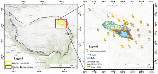
Figure 1.
Overview of the Study Area.
2.2. Data Sources and Processing
The precipitation observations used in this study were obtained from three ground-based monitoring networks: (1) Twenty daily-scale rain gauges from the National Meteorological Information Center (NMIC), comprising nine stations (Tuole, Yeniugou, Qilian, Delingha, Gangcha, Menyuan, Wulan, Chaika, Shandan) spanning 2001–2017 and eleven stations extending through 2020; (2) Nine high-frequency stations (with 10 min/30 min sampling intervals) from the HeiHe River Basin Observational Network [39], operational between 2013 and 2020; (3) Two wetland meteorological stations (Wayanshan and Xiaopohu) maintained by Qinghai Normal University, providing 30 min resolution data during 2017–2019. All station data were rigorously quality-controlled, with outliers removed prior to their use in evaluating gridded precipitation datasets.
The Global Precipitation Measurement (GPM) mission, representing a paradigm shift in spaceborne precipitation retrieval [35], provides the foundational data for this study through its Level-3 Final Multi-satellite Integrated Product (officially designated GPM_3IMERGDE_07). A critical advancement is the Dual-frequency Precipitation Radar (DPR) system that substantially enhances detection sensitivity for light precipitation (0.2 to 0.5 mm·h−1) and solid-phase hydrometeors (snow, graupel, etc.), achieving 0.1 mm·h−1 radiometric resolution through Ka/Ku-band synergy. Numerous studies have demonstrated its reliable performance in meteorological and hydrological applications across the Tibetan Plateau region [40,41,42], making it particularly suitable for modeling in the Qinghai Lake Basin where solid precipitation dominates during cold seasons. The full name of this data product is GPM IMERG Final Precipitation L3 1 day 0.1° × 0.1° V07. It has a daily temporal resolution, and the data format is NetCDF. This study covers the period from 2001 to 2020. The preprocessing steps include converting HDF files to TIF, projection transformation, cropping, and calculating monthly and annual precipitation.
The Normalized Difference Vegetation Index (NDVI), a widely recognized biophysical proxy in precipitation downscaling research [43], The dataset used in this study was provided by Gao et al. [44], integrates satellite observations with land use data through monthly maximum value composites at 16-day intervals. Covering 2001–2020 with 250 m spatial resolution, the dataset contains 12 annual periods (monthly composites) that were preprocessed through coordinate system conversion, spatial subsetting, and resampling to ensure consistency with other geospatial inputs. Topographic determinants, critical for orographic precipitation modulation [45], and Shuttle Radar Topography Mission (SRTM) Digital Elevation Model (DEM) at 90 m spatial resolution were used, and ArcGIS 10.7 was used to obtain the terrain derivatives (slope gradient and aspect) and geographic coordinates (longitude, latitude). Consequently, the NDVI, DEM, SLOPE, ASPECT, longitude, and latitude data for the study area were acquired at both 0.1° × 0.1° and 0.01° × 0.01° grid resolutions.
2.3. Downscaling Methodology and Residual Correction
The core principle of statistical downscaling lies in modeling the relationship between precipitation and surface predictor variables (e.g., NDVI, DEM) at a coarse spatial resolution (0.1° × 0.1°), and extrapolating this relationship to finer resolutions (0.01° × 0.01°) [13]. In this study, NDVI, DEM, slope, and aspect were selected as surface descriptors [46], while longitude and latitude were incorporated as additional spatial predictors [47]. Machine-learning regression models were employed to capture the nonlinear mapping between precipitation and surface characteristics. High-resolution downscaling was achieved by applying the trained models to the 0.01° surface feature grids. To further improve accuracy, a residual correction step was introduced to account for precipitation variability not captured by the models [31]. First, precipitation estimates at 0.1° resolution were obtained from the downscaling models. Residuals were computed by subtracting the original GPM 0.1° precipitation values from the predicted 0.1° outputs. These residuals were then interpolated from 0.1° to 0.01° resolution using bilinear interpolation. Finally, the interpolated residuals were added to the 0.01° downscaled precipitation outputs to obtain the corrected high-resolution precipitation fields. The complete downscaling and residual correction workflow is illustrated in Figure 2.
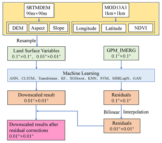
Figure 2.
Workflow of Downscaling and Residual Correction Techniques.
2.4. Machine-Learning Algorithms
This study employs a diverse suite of nine machine-learning algorithms, encompassing both conventional and deep-learning approaches, to systematically evaluate their precipitation downscaling efficacy in the Qinghai Lake Basin. The selected algorithms are categorized as follows:
1. ANN
The Artificial Neural Network (ANN) employs a three-layer feed-forward structure (input-hidden-output) with hyperbolic tangent activation functions to capture nonlinear precipitation-topography relationships [48]. During training, the discrepancy between predicted and actual values is continuously compared; errors are backpropagated to update network weights, thereby optimizing downscaling accuracy. This architecture offers advantages in simplicity, fast training speed, intuitive model construction, and relatively straightforward parameter tuning [31]. However, its capability for modeling sequential data is limited, and capturing spatiotemporal dependencies represents a significant weakness [49]. The initial learning rate is set to 0.0001, Epsilon to 1 × 10⁻⁸, and the Adam optimizer is combined with dynamic learning rate scheduling. The maximum number of training epochs is 300, samples are randomly shuffled within each iteration, and the optimization tolerance threshold is 1 × 10⁻⁴. The data is partitioned into 80% for training, 10% for validation, and 10% for testing.
2. CLSTM
The CNN-LSTM (CLSTM) architecture synergizes Convolutional Neural Networks (CNN) and Long Short-Term Memory (LSTM) networks to achieve high-precision precipitation downscaling through multi-scale feature extraction and spatiotemporal dependency modeling [50]. Its core strength lies in exceptional spatiotemporal feature fusion capability [51]: CNNs precisely extract spatial pattern features (e.g., elevation transition zones, lake boundaries) from topography and vegetation data, while LSTMs effectively model the temporal evolution of precipitation processes. This synergy optimizes the dynamic response mechanism between terrain and precipitation. The gating mechanisms (forget gate/input gate) enable precise capture of long- and short-term dependencies through selective memorization [52], and the architecture facilitates the integration of multi-source heterogeneous data (e.g., satellite imagery, terrain data, surface features) via parallel processing [53]. It comprises a multi-modal feature input layer, spatial feature extraction module, temporal dependency modeling module, and multi-task output layer, jointly addressing terrain characteristics and precipitation processes. The optimizer is Adam with an initial learning rate of 0.0005 and epsilon of 1 × 10⁻⁸. A dynamically weighted Mean Squared Error (MSE) loss function is employed, assigning higher weights to high-precipitation events to enhance the model’s capability in reconstructing extreme precipitation events [54]. However, the model exhibits high training complexity and significant computational resource demands [55,56]. The data is partitioned into 70% training, 15% validation, and 15% testing sets.
3. Transformer
The Transformer, combined with CNNs, leverages a global attention mechanism synergized with local feature extraction. This integration enhances modeling capability in complex terrains, enabling high-precision spatiotemporal downscaling of precipitation data [33]. The global attention mechanism excels at capturing long-range spatial dependencies, and parallel computation accelerates the training process [57,58]. However, the model possesses a vast number of parameters, requires substantial GPU memory, and exhibits limitations in extracting localized features [59,60]. The optimizer is Adam with an initial learning rate of 0.0001 and epsilon of 1 × 10⁻⁸, incorporating a dynamic learning rate adjustment strategy: the learning rate is halved if the validation loss shows no improvement for five consecutive epochs, with a minimum learning rate of 1 × 10⁻⁶ to prevent the model from converging to a local overfit. The data is partitioned into 90% training, 5% validation, and 5% testing sets.
4. RF
Random Forest (RF) is a nonlinear regression method based on ensemble learning, which achieves highly robust modeling by aggregating predictions from multiple decision trees [61]. The algorithm demonstrates strong robustness, enabling it to effectively resist noise and outlier interference, and offers good interpretability through feature importance selection [62]. In this study, an improved RF algorithm was adopted. A downscaling model for precipitation data was developed through feature importance analysis and hyperparameter optimization. Each decision tree employs the CART algorithm, selecting split features by minimizing Gini impurity and incorporating a random feature selection mechanism. This automatic hyperparameter search facilitates an adaptive parameter model. However, RF exhibits substantial memory consumption with high-dimensional data, limiting its applicability to large-scale problems. Additionally, it is prone to underestimating extreme precipitation events and inadequately characterizing intense rainfall processes [63,64]. A total of 500 unpruned decision trees were constructed, enhanced by the random feature selection mechanism. The data is partitioned into 80% for training and 20% for testing.
5. XGBoost
Extreme Gradient Boosting (XGBoost) integrates multiple CART regression trees within a gradient-boosting framework, constraining model complexity through leaf-node weight regularization and feature subsampling [65]. This approach enhances model capacity, spatial representation, and generalization ability. Crucially, XGBoost supports parallel computation, significantly improving computational efficiency compared to traditional RF while consuming fewer resources [66]. However, its hyperparameter tuning is complex and requires meticulous adjustment to avoid suboptimal solutions [67]. In this study, a random search was employed for hyperparameter optimization, focusing on key parameters: a tree depth of 9, a learning rate of 0.1, and a column sampling rate of 0.8. Ultimately, 500 depth-constrained boosted trees were selected. The data is partitioned into 80% for training and 20% for testing.
6. KNN
The K-Nearest Neighbors (KNN) algorithm predicts target values by averaging (weighted or unweighted) the values of the k-nearest training samples within a multidimensional feature space [68]. Predictions rely on local neighborhood samples, avoiding global model bias. The model demonstrates good compatibility with geospatial analysis [69]. However, computational complexity increases exponentially with data volume, model performance degrades significantly with high-dimensional features, and it is susceptible to interference from irrelevant variables [70,71]. In this study, Bayesian optimization replaced traditional hyperparameter search methods to explore optimal configurations more efficiently. Thirty optimization iterations were performed, with model performance evaluated using 5-fold cross-validation and negative mean squared error as the objective function. The data is partitioned into 80% for training, 5% for validation, and 15% for testing.
7. SVM
The Support Vector Machine (SVM) constructs a hyperplane in a high-dimensional feature space that tolerates deviations within a specified ε margin, ensuring prediction errors for all samples remain within ε [72]. SVM excels in high-dimensional spaces, and its kernel functions offer flexibility in adapting to complex nonlinear relationships [73]. However, training speed and scalability decrease significantly as data volume increases [74,75]. In this study, the radial basis function (RBF) kernel was employed to effectively capture complex relationships between precipitation and environmental factors (e.g., topography and vegetation). The kernel parameter was set to ‘scale’, which is automatically adjusted based on feature count and variance, enhancing model adaptability to diverse datasets. The data was partitioned into 80% for training and 20% for testing.
8. MSRLapN
The Multi-Scale Residual Laplacian Network (MSRLapN), based on the ResLap architecture, incorporates residual learning. It extracts multi-scale features in parallel using convolutional layers with varying dilation rates and preserves high-resolution details by integrating attention mechanisms and skip connections [32]. This architecture enhances the representation of complex climate features. Residual connections effectively alleviate the vanishing gradient problem and improve stability in deep networks [76,77]. The multi-scale residual network significantly boosts feature extraction capability. However, increasing network depth leads to longer training times [78]. The data was partitioned into 70% for training, 15% for validation, and 15% for testing.
9. GAN
Generative Adversarial Networks (GANs) learn the mapping between feature inputs and precipitation through adversarial training of a generator and a discriminator [79]. Generated precipitation data exhibit spatial distribution patterns consistent with meteorological principles and are recommended for simulating extreme weather events [80]. In this study, the Wasserstein distance replaced the traditional Jensen-Shannon (JS) divergence. A gradient penalty was introduced to enforce the Lipschitz continuity constraint, stabilizing the training process. This approach effectively addressed the mode collapse issue in traditional GANs and demonstrated superior performance on multiple evaluation metrics [81]. However, training instability persists, and balancing the generator and discriminator for effective convergence control presents significant challenges [82,83]. The data was partitioned into 80% for training, 10% for validation, and 10% for testing.
2.5. Validation
The evaluation consists of two components: (1) validation of the model’s performance and (2) assessment of the accuracy of the downscaled precipitation dataset.
2.5.1. Model Performance Validation
K-fold cross-validation is a widely used method for evaluating model performance by repeatedly partitioning the dataset [84]. The dataset is evenly divided into K subsets. In each iteration, one subset is used as the validation set while the remaining K−1 subset is used for training. This process is repeated K times, and the average of the K validation results is used as the final performance metric. Building on this, Rodriguez et al. [85] analyzed the sources of variance in cross-validation, and Fushiki et al. [86] examined the impact of different K values on estimation bias. These contributions significantly enhance the reliability of model evaluation [87]. Selecting a smaller K value represents a trade-off between computational efficiency and evaluation stability.
K-fold cross-validation helps to accurately assess model performance, mitigates overfitting, and enhances the generalization capability of the precipitation prediction model. In this study, the evaluation metrics used include Coefficient of determination (R2), Bias, Sigma Ratio, Mean Absolute Error (MAE), Centered Root Mean Square Error (CRMSE), and Root Mean Square Error (RMSE).
2.5.2. Accuracy Assessment of Downscaled Precipitation Datasets
While the optimal model can be identified through performance validation at a given spatial resolution, the high-resolution precipitation data obtained from downscaling must be further evaluated against ground-based rain gauge observations. In this study, seven commonly used evaluation metrics were employed: correlation coefficient (CC), RMSE, MAE, R2, Sigma Ratio, Kling-Gupta Efficiency (KGE), and Bias.
2.5.3. Formulations
1. Correlation Coefficient (CC)
2. Root Mean Square Error (RMSE)
3. Mean Absolute Error (MAE)
4. Coefficient of Determination (R2)
5. Sigma Ratio (Standard Deviation Ratio)
6. Kling-Gupta Efficiency (KGE)
7. Bias
8. Corrected Root Mean Square Error (CRMSE)
where is the observation measured by station , is the precipitation estimated by a model at the location of station , is the mean value of all station observations, and is the mean value of the estimated precipitation at all the locations with stations. is the Standard deviation of observed values, and is the Standard deviation of predicted values.
3. Results
3.1. Model Performance Assessment
To conduct a preliminary assessment of model performance, nine machine-learning algorithms were applied to reconstruct precipitation data at a spatial resolution of 0.1° for the period 2001–2020, without implementing any spatial downscaling. This procedure served to evaluate the intrinsic reconstruction capabilities of each algorithm and to screen suitable candidates for subsequent downscaling tasks. The performance evaluation metrics for each algorithm are shown in Figure 3, while the predicted spatial precipitation distributions for the year 2005 are illustrated in Figure 4.
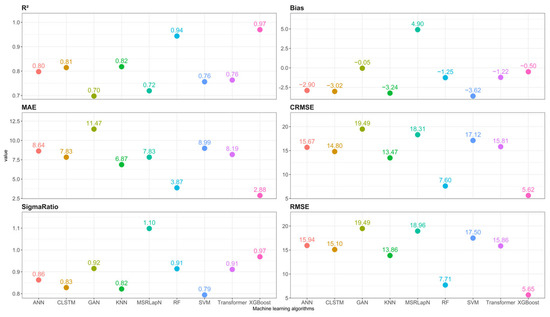
Figure 3.
Evaluation metrics of model performance in precipitation prediction.
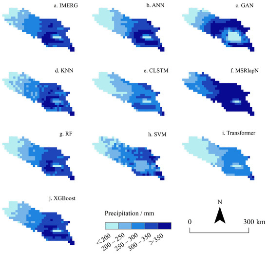
Figure 4.
Spatial distribution of model-predicted precipitation in 2005.
It is evident from the results that XGBoost outperformed all other models, followed closely by RF, as indicated by R2 values of 0.97 and 0.94, biases of −0.5 mm and −1.25 mm, MAE of 2.88 mm and 3.87 mm, and RMSE of 5.65 mm and 7.71 mm, respectively. These metrics collectively suggest that both models exhibit minimal underestimation and high stability, with strong performance in capturing precipitation variability, as demonstrated by SigmaRatio values of 0.97 and 0.91, respectively. In addition, their spatial distribution patterns align closely with the 0.1° GPM dataset.
Although the GAN model produced the lowest bias (−0.05 mm), it exhibited substantial variability in its predictions (MAE = 11.47 mm, RMSE = 19.49 mm), with spatial outputs showing alternating regions of high and low values. Transformer, generated an overly smoothed spatial trend, failing to effectively capture variations in high-value regions—a trend that can be attributed to its significant underestimation, as evidenced by the largest bias (−3.62 mm). The ANN, SVM, KNN, and CLSTM consistently underestimated precipitation, with biases ranging from −2.9 mm to −3.62 mm and RMSEs between 13.86 mm and 15.94 mm. MSRLapN was the only model to overestimate precipitation (bias = 4.90 mm), showing a marked deviation from observed values (RMSE = 18.96 mm) and a spatial pattern indicative of high-value region diffusion.
3.2. Precision Assessment of Downscaled Precipitation Datasets
Figure 5 and Figure 6 illustrate the spatial distribution of precipitation products over the Qinghai Lake Basin before and after downscaling calibration using nine machine-learning methods. The coarse-resolution original data (Figure 4a) revealed noticeable gaps along the basin boundaries and demonstrated limited capability in capturing precipitation gradients, primarily attributed to the coarse pixel size and satellite bandgap effects. Among the uncalibrated models, the Transformer exhibited the poorest performance in capturing high-precipitation zones (>490 mm), with a significant underestimation (Bias = −7.38 mm). Similarly, CLSTM also underestimated precipitation in high-value areas (Bias = −4.08 mm and −6.72 mm), and the resulting image lacked smooth transitional features. Moreover, the spatial variance of the GAN model was overly amplified (Sigma Ratio = 1.037), indicating instability in representing spatial patterns. In contrast, the remaining methods enhanced the representation of spatial details and coverage, while preserving the spatial distribution characteristics of the original dataset. However, performance differences in spatial representation accuracy remain evident.
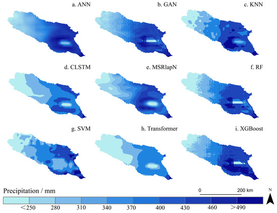
Figure 5.
Spatial distribution of downscaled precipitation at 0.01° resolution in 2005, prior to calibration, using nine machine-learning algorithms.
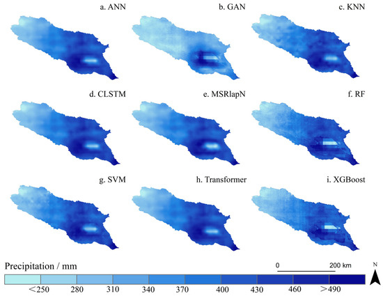
Figure 6.
Spatial distribution of downscaled precipitation at 0.01° resolution in 2005, after calibration, using nine machine-learning algorithms.
Validation using surface rain gauge data from 26 stations (Figure 7) revealed that the raw GPM dataset has limited accuracy, with an R2 of 0.72 and an RMSE of 17.78 mm. Notably, several machine-learning-based downscaling models demonstrated competitive performance even prior to calibration. Among the uncalibrated models, KNN achieved the best performance, with an R2 of 0.75—surpassing that of the original dataset. The RF model exhibited error levels like the raw GPM data (RMSE = 19.80 mm, R2 = 0.67). In contrast, some models showed limited predictive capability. For instance, the Transformer algorithm yielded a relatively low KGE of 0.58, with a Bias of −7.38 mm and a Sigma Ratio of 0.74, clearly underperforming relative to other models.
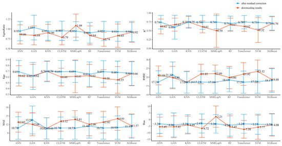
Figure 7.
Comparison of evaluation metrics before and after residual correction for nine ML-based downscaling methods.
After calibration, most models exhibited enhanced performance. For KNN, the Bias decreased from −4.09 mm to −3.31 mm (a 19% reduction), accompanied by an RMSE of 17.09 mm and a KGE of 0.697, making it the best-performing model. XGBoost improved its capacity to capture spatial variability, as indicated by a 0.02 increase in Sigma Ratio, and achieved an RMSE of 18.17 mm and an R2 of 0.71—both better than in its uncalibrated form. CLSTM effectively reduced its Bias from −6.72 mm to −2.97 mm, with the KGE increasing to 0.69. Transformer also demonstrated substantial improvement, achieving a 56.1% reduction in Bias and an RMSE of 17.21 mm—comparable to KNN. For ANN, the Bias was reduced by 39.7% to −3.28 mm, and the KGE increased by 0.13; however, its R2 remained slightly below that of KNN, at 0.74. The SVM model also exhibited a 0.13 increase in KGE. MSRLapN and RF experienced moderate improvements, as evidenced by reduced errors and enhanced model interpretability. In contrast, the GAN model performed worse after calibration: its explanatory power declined (R2 dropped to 0.59), and both RMSE and MAE increased to 21.32 mm and 13.58 mm, respectively—indicating a further degradation in predictive accuracy.
3.3. Performance of Cold and Warm Seasons
The Qinghai Lake Basin exhibits distinct seasonal precipitation characteristics, with cold-season (October-April) precipitation primarily in solid form and warm-season (May-September) precipitation dominated by liquid form [88]. In the cold season, precipitation is relatively low, predominantly in solid form, whereas the warm season receives more precipitation, mainly as rainfall. Accordingly, a multidimensional assessment of the seasonal downscaling performance was conducted using ground-based rain gauge observations (Figure 8 and Figure 9).
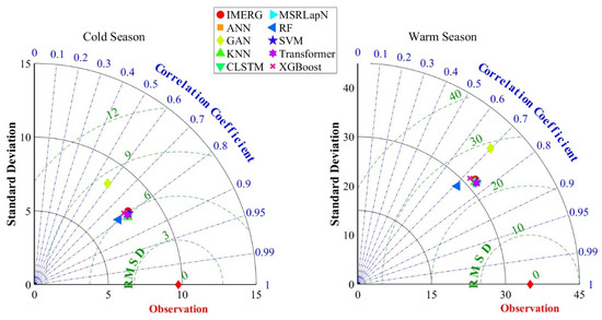
Figure 8.
Taylor Diagram for the Calibration of Precipitation Datasets in the Cold and Warm Seasons Based on Ground-Based Observations.
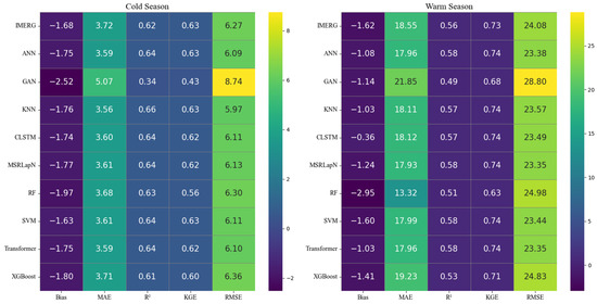
Figure 9.
Heatmap for the Calibration of Precipitation Datasets in the Cold and Warm Seasons Based on Ground-Based Observations.
During the cold season, KNN demonstrated the best downscaling performance, with a 3.1% improvement in CC compared to the original data, a 5.4% reduction in CRMSE, a 4.3% decrease in MAE, and optimal values in both KGE and RMSE. The Taylor diagram (Figure 8 and Figure 9) indicates that KNN most accurately replicates the spatial heterogeneity and variability trends of cold-season precipitation (SD closest to observed, highest CC), suggesting its stronger capability for predicting snow and freezing precipitation. ANN exhibited the highest sensitivity to precipitation fluctuations in the cold season (Sigma Ratio = 0.81), reflected in the Taylor diagram by an SD ratio close to 1. This indicates ANN’s relative strength in capturing the amplitude and fluctuation characteristics of precipitation, highlighting its potential advantage in predicting spatiotemporal variations during the cold season. In the warm season, Transformer outperformed the raw data with consistently higher CC values (up to 0.76), a 3.0% reduction in CRMSE, and a 17.7% improvement in KGE. Its excellent Taylor diagram performance (higher CC, lower CRMSE) further demonstrates its robust ability to capture the spatial distribution and intensity of predominantly rainfall-driven precipitation. Other models showed varied sensitivity to seasonal precipitation patterns. SVM performed well in the warm season (CC = 0.76, KGE = 0.74), and its relative error rate (MAE/observations) was 29.8%, lower than that in the cold season (53.3%). XGBoost achieved a 1.0% reduction in RMSE in the warm season (24.83 mm) and a 17.8% decrease in cold-season RMSE (6.36 mm). RF showed better feature consistency in the cold season (CC = 0.79) than in the warm season (0.71) and exhibited the highest standard deviation ratio error in the warm season, exceeding the original data by 18.8%.
The raw IMERG data did not perform well in either season, ranking fifth in the cold season (σ = 0.8256), and in the warm season, its RMSE (24.08 mm) was 3.0% higher than the best-performing model (MSRLapN). Most ML-based downscaling methods (e.g., KNN, MSRLapN) enhanced the ability to capture seasonal precipitation patterns through feature optimization and calibration incorporating surface predictors. However, the GAN model performed poorly in both seasons (e.g., the cold-season CC was 25.47% lower than the original, and the warm-season RMSE increased by 19.87%). Correspondingly, its points in the Taylor diagrams for both seasons lie considerably farther from the observed gauge reference, implying limitations in its applicability for precipitation downscaling over complex terrain. These findings underscore the importance of accounting for seasonal differences in precipitation downscaling and demonstrate that most machine-learning models—especially when calibrated—can improve spatial representation in both cold and warm seasons, although their sensitivity and adaptability depend on algorithmic characteristics.
4. Discussion
4.1. Value of ML Downscaling
The results in Section 3.2 demonstrate that the machine-learning-based downscaling frameworks effectively enhance precipitation estimation accuracy while preserving spatial coherence and reconstructing high-resolution precipitation patterns. However, there are differences in the spatial performance of different models, and the evaluation metrics combined with rain gauge precipitation data show that the four approaches—KNN, SVM, ANN, and Transformer—exhibit varying levels of performance across both annual and seasonal scales. To better identify the optimal downscaling method for the Qinghai Lake Basin, precipitation event intensities were categorized using quintiles [89]. The quantile-based validation results (Figure 10 and Figure 11) reveal distinct model characteristics: KNN demonstrated exceptional performance in predicting low-precipitation events (0–40%). At 0%, it achieved the lowest MAE (4.35 ± 0.41 mm) and RMSE (7.75 ± 0.55 mm) among all models. This superiority persisted at 20% for both MAE (4.63 ± 0.45 mm) and RMSE (8.32 ± 0.94 mm). At 40%, KNN maintained the lead in MAE (4.54 ± 0.40 mm) and exhibited the smallest error standard deviation across all models. The boxplots further indicated the most compact error distribution for KNN, reflected by the narrowest interquartile range (IQR) compared to SVM and ANN. In contrast, while Transformer did not exhibit absolute dominance at any single percentile, it showed the smallest fluctuation in RMSE across all percentiles (with a standard deviation approximately 15% lower on average than KNN). Concurrently, the Transformer displayed the most compact boxplots (smallest IQR) and the fewest outliers across different percentiles, suggesting potential advantages in overall stability. SVM and ANN showed notable performance only at specific percentiles (e.g., SVM had a lower MRE% at the 0th percentile, while ANN showed relatively stable errors at 60%).
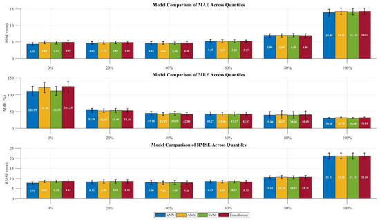
Figure 10.
Comparison of error metrics across precipitation intensity quantiles for different models.
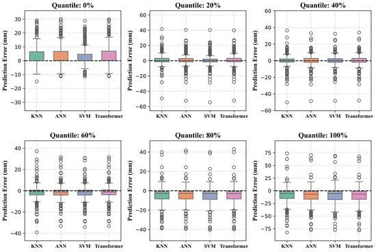
Figure 11.
Error distribution characteristics across precipitation intensity quantiles for different models.
Figure 12 shows that although all four approaches can resolve orographic gradients of low-resolution data for intra-basin applications, KNN (Figure 12b) and SVM (Figure 12c) are better able to capture the spatial gradient variations in precipitation compared to ANN (Figure 12d) and Transformer (Figure 12e), and the two deep-learning approaches, ANN, and Transformer, perform spatially with a spatial detail attenuation, while SVM has more instability than KNN. Based on a comprehensive assessment involving both spatial pattern representation and rain gauge validation, KNN emerges as the most suitable downscaling method for IMERG precipitation in the Qinghai Lake Basin.
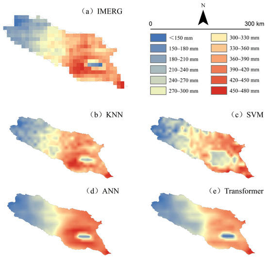
Figure 12.
Spatial Distribution Patterns of Four Precipitation Products (2005).
In summary, the machine-learning downscaling technique based on surface characteristics (NDVI, DEM, SLOPE, ASPECT, latitude, longitude), combined with residual correction, can generate higher resolution precipitation data, which can provide 0.01° precipitation products for watershed hydrological research and water resource management.
4.2. Residual Analysis
The application of residual correction to the downscaled precipitation datasets showed improved accuracy across all eight machine-learning models, except for GAN. To further explore the mechanisms through which residual correction influences model performance, we calculated and visualized the 20-year mean annual residual distribution (Figure 13), where positive values indicate underestimation and negative values indicate overestimation. In conjunction with the evaluation results before and after calibration (Figure 7), GAN exhibited the maximum residual range of 332.91 mm, showing severe underestimation near lake margins and overestimation along watershed boundaries. KNN displayed the smallest residual range [−20.61 mm, 28.59 mm] throughout the basin, resulting in the highest model accuracy after calibration. The consistently positive residuals of the Transformer align with its downscaling performance (with a bias of −7.38 mm, the smallest absolute value among all methods). Although SVM showed the second-largest residual range (263.42 mm), its modeling performance still benefited from residual correction. The residuals for ANN (range: 49.49 mm) were distributed along both lake shores and watershed boundaries. All other methods exhibited smaller residual ranges than GAN, with high residual magnitudes (absolute values) predominantly clustered near lakeshores, suggesting persistent challenges in accurately modeling precipitation near lake margins.
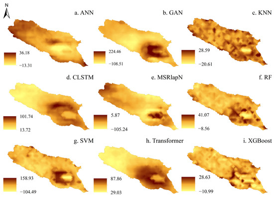
Figure 13.
Spatial Distribution of Residual Mean for Nine ML Methods over 20 Years.
These findings demonstrate that both the spatial distribution and magnitude range of residuals directly determine calibration effectiveness. The residual magnitude range must remain within model-specific thresholds; exceeding these thresholds may reduce calibration efficacy or even degrade model accuracy (as observed with GAN). Different models exhibit varying threshold requirements, emphasizing the necessity of model-specific calibration strategies. Moreover, due to the inherent characteristics of the GAN model during network generation (explicit noise input) [90], during the residual correction process, when upscaling 0.1° residuals to 0.01° resolution using bilinear interpolation, not only were the genuine error signals amplified, but the noise components within them were also amplified. Particularly in mountainous regions with complex terrain, this linear interpolation approach may fail to accurately capture the nonlinear relationship between precipitation errors and topography (such as windward/leeward effects) [91], further leading to the mode collapse observed in the GAN’s residual correction.
4.3. Limitations and Prospects
KNN demonstrated optimal performance in downscaling IMERG precipitation products within the Qinghai Lake Basin. The calibrated KNN model (CC = 0.92, RMSE = 17.09 mm, KGE = 0.70) outperformed the original dataset, particularly achieving the lowest MAE (10.62 mm) during cold seasons, representing a 4.3% improvement over the original data. This suggests a superior ability to predict low-precipitation values compared to other models.
The method effectively captures spatial precipitation details across both high-value central basin areas and low-value boundary regions, a characteristic attributable to its nonparametric locally weighted learning approach [92]. Furthermore, since the KNN algorithm relies on feature space similarity [69], it can generate similar precipitation conditions in analogous geographical environments. This explains its enhanced performance during cold seasons when precipitation patterns are relatively stable. However, during warm seasons, the complex nonlinear relationships of convective precipitation and high stochasticity of local microclimates [93] pose challenges to KNN predictions, resulting in their seasonally varying applicability (inferior performance in warm seasons). Despite KNN’s overall superiority, residual analysis revealed sensitivity to data noise, with model performance potentially compromised under conditions of high-precipitation variability or extreme meteorological events, as evidenced by its second-ranked warm-season performance. This further indicates that the model’s predictions may be affected during periods of substantial precipitation variation or extreme climate conditions. While its excellent performance in low-intensity precipitation events suggests suitability for long-term precipitation monitoring within the basin, future research should address the model’s adaptability under extreme climate scenarios.
The Transformer architecture demonstrated the second-best comprehensive downscaling performance among deep-learning approaches. While exhibiting significant underestimation prior to calibration (Bias = −7.38 mm), post-calibration refinement substantially improved model performance (Bias = −3.24 mm, RMSE = 17.21 mm). Although slightly inferior to KNN, the observed metric differences proved statistically insignificant—exhibiting a minimal KGE difference of 0.01 and an RMSE increase of merely 0.11 mm. This indicates that the global attention mechanism exhibits strong compatibility with residual correction techniques, while also demonstrating better overall stability and less fluctuation in prediction errors. However, its spatial detail representation (e.g., precipitation gradients and local variations) appears relatively smooth, resulting in a moderately weaker capability to capture subtle local changes. Conversely, this characteristic suggests the model possesses significant potential for future applications in attributing extreme events under climate change scenarios. This finding suggests two critical insights: (1) the global attention mechanism demonstrates strong synergy with residual correction techniques, and (2) the architecture exhibits considerable potential for future implementation in precipitation downscaling applications. During experimental evaluation, we observed that the Transformer model is prone to overfitting during prediction. The current model may be overfitting to typical precipitation patterns. Although this can be mitigated by reducing the number of multi-head attention layers and finetuning hyperparameters, it remains essential to strike a balance between model accuracy and the risk of overfitting.
This study employed six carefully selected features (longitude, latitude, NDVI, DEM, slope, and aspect) that demonstrate strong physical relationships with precipitation distribution. The models achieved significant learning effectiveness (with R2 > 0.70 for all methods except GAN), while the generally low residual values across the basin further confirm that these six features effectively capture the spatial heterogeneity of precipitation during the downscaling process. SHAP analysis was conducted on six geospatial predictors (Longitude, Latitude, NDVI, DEM, Slope, Aspect) across four machine-learning architectures (ANN, KNN, SVM, Transformer), as illustrated in Figure 14a–d. Algorithmic disparities yielded divergent feature importance profiles, consequently affecting model performance and spatial downscaling fidelity. The Transformer architecture demonstrated dependence on topographic features (Aspect, DEM, and NDVI ranked top three in contribution), resulting in excessively smoothed spatial patterns that neglected precipitation heterogeneity—a likely consequence of its global attention mechanism prioritizing regional trends over local variations.
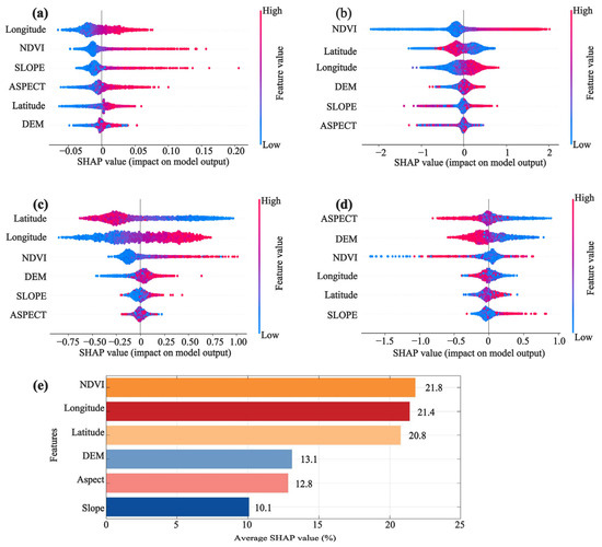
Figure 14.
SHAP analysis results for selected models: (a) ANN, (b) KNN, (c) SVM, (d) Transformer, and (e) average feature importance across models.
Three dominant predictors emerged across all models (Figure 14e): (1) NDVI, (2) Latitude, and (3) Longitude. NDVI, an important parameter characterizing vegetation growth, is strongly correlated with rainfall [36,94,95]. It also influences atmospheric sensible and latent heat fluxes, which directly affect near-surface temperature and moist convection [96], thereby impacting precipitation. Latitude and longitude are key indicators of land–sea configuration. Generally, higher eastern longitudes and lower latitudes are associated with greater precipitation. Geographically, latitude and longitude fundamentally influence land–sea thermal contrasts by modulating solar radiation distribution and monsoonal pathways, thereby shaping regional precipitation regimes. However, the relationship between precipitation and NDVI is susceptible to anthropogenic influences [45]. This is particularly evident in the Qinghai Lake Basin, where human activities are predominantly concentrated along the lakeshore. These areas are mainly covered by sand, resulting in a relatively limited impact of precipitation on NDVI, which may partly explain the concentration of residuals near the lakeshore. Future research should explore additional environmental variables to optimize the selection of predictor variables and enhance model performance.
As shown in the results of Section 3.1, the superior learning performance of XGBoost compared to other models can be primarily attributed to its gradient-boosting ensemble framework [97]. This framework iteratively combines multiple weak learners (decision trees) and continuously corrects the prediction errors of preceding models to ultimately construct a high-accuracy strong predictor. The tree-based structure excels at capturing complex nonlinear relationships and interactions among features [98]. Importantly, XGBoost incorporates built-in L1/L2 regularization to effectively mitigate overfitting, thereby significantly enhancing the model’s generalization capability [99]. Additionally, its inherent capability for automatic feature selection allows it to focus on the most relevant features [100] and confers a degree of robustness to the feature scale [101]. Furthermore, XGBoost demonstrates superior adaptability to imbalanced datasets, such as those involving extreme precipitation events [102], which is particularly relevant in precipitation downscaling tasks. These combined characteristics contribute to the more stable predictive performance exhibited by XGBoost in this study. It is worth noting that the Random Forest (RF) model, which is also based on a tree structure, showed the second-best learning performance. However, it is crucial to recognize that learning represents only one phase of the downscaling workflow. The learning effectiveness demonstrated during this phase does not fully represent the overall model performance. Therefore, a comprehensive evaluation incorporating multiple dimensions remains essential for assessing model applicability.
Analysis revealed that all machine-learning models exhibited relatively poorer performance in estimating precipitation over water bodies compared to terrestrial areas. This limitation primarily stems from two factors: (1) inherent constraints in satellite-based precipitation estimation over aquatic surfaces [103,104], and (2) information loss during the upscaling process of high-resolution input features, particularly pronounced in complex mountainous terrain [45]. These factors collectively degraded model learning efficacy. Furthermore, our results align with existing findings that traditional algorithms like Random Forest (RF) and XGBoost experience accuracy deterioration and noise amplification when applied to downscaling in topographically complex mountainous regions [105].
Specifically, the residual correction was applied to improve model accuracy. However, such correction is not universally effective—for instance, in the case of the GAN model—since its performance is constrained by model-specific threshold values. Tailored correction strategies may be necessary, depending on the unique characteristics of each model. Additionally, the potential influence of alternative interpolation methods on the effectiveness of residual correction warrants further investigation. Specifically, to address the mode collapse in the GAN correction, future research will consider introducing physically constrained interpolation during its correction process [106], constructing terrain gradient weighting functions, and using the topographic physical attributes from the digital elevation model (DEM) as guiding factors for the interpolation process [107]. This physics-guided interpolation method essentially integrates data-driven techniques with atmospheric topographic dynamics principles [108]. By endowing the DEM with physical meaning, the correction process follows the principle that “the more complex the terrain, the stronger the nonlinearity of the interpolation should be” [109], aiming to improve the GAN’s model performance in complex terrain regions. Although monthly precipitation data were derived from daily observations, short-duration, and high-frequency precipitation events were inevitably overlooked. Future research should consider employing higher temporal-resolution datasets. While increasing the dimensionality of the input data [27] may enhance model performance, it also imposes greater computational costs. Therefore, the adoption of high-performance computing resources is recommended to support high-resolution precipitation forecasting.
Evaluation results indicate that each algorithm exhibits distinct advantages. For instance, RF demonstrates robustness to outliers, while Transformer models excel in extracting discriminative spatial-temporal patterns, ANN effectively captures nonlinear relationships between environmental predictors and precipitation distributions, and XGBoost exhibits the highest model stability. Consequently, determining how to select and integrate different algorithms based on specific application needs will be a key focus in future research [110].
5. Conclusions
This study applies nine machine-learning algorithms to spatially downscale IMERG precipitation data from 0.1° to 0.01° resolution in the Qinghai Lake Basin. Incorporating a deep-learning framework into the evaluation system, model performance was rigorously evaluated against gauge precipitation data to assess differences among models. Results indicate that the calibrated KNN demonstrated superior comprehensive performance. The machine-learning downscaling approach effectively preserved the spatial coherence of precipitation data while capturing critical gradient features. Residual correction improved the performance of all models except GAN, indicating its general effectiveness. NDVI emerged as the most influential predictor; however, its effectiveness was limited by anthropogenic disturbances and heterogeneous land cover types such as bare soil and sandy areas, highlighting the need to optimize input feature selection. Based on the proposed downscaling framework, this study produced optimal spatially downscaled precipitation results, well-suited for applications in the Qinghai Lake Basin that require high-resolution precipitation data.
These results are well-suited for applications within the basin requiring high-resolution precipitation data and offer a selection basis for downscaling techniques in complex alpine mountainous regions. However, the transferability and stability of the developed models to other regions with different characteristics require further evaluation. Developing algorithms that integrate outputs or features from multiple models will be a key focus of future work. Furthermore, advancing downscaling techniques at higher temporal resolutions and generating corresponding precipitation datasets will be of great significance for hydrological and ecological research.
Author Contributions
Conceptualization, K.L. and L.Z.; methodology, K.L., L.Z., and L.G.; supervision, L.Z.; validation, K.L. and L.Z.; formal analysis, K.L. and L.Z.; writing—original draft preparation, K.L.; writing—review, and editing, K.L., L.Z., and L.G. All authors have read and agreed to the published version of the manuscript.
Funding
The research is supported by the National Natural Science Foundation of China (42171467); and the Natural Science Foundation of Qinghai Province (2022-ZJ-711).
Data Availability Statement
The raw data supporting the conclusions of this article will be made available by the authors on request.
Acknowledgments
The datasets supporting this study are publicly available from the following sources: Gauge precipitation data: (1) China Meteorological Administration (CMA): http://data.cma.cn, accessed on 29 July 2022; (2) National Tibetan Plateau Data Center (TPDC): https://data.tpdc.ac.cn/, accessed on 15 November 2024; (3) Wayanshan and Xiaopohu Wetland Observatory (Qinghai Normal University): Available upon request from the corresponding author. GPM_IMERG satellite precipitation data: NASA Earth data: https://search.earthdata.nasa.gov, accessed on 18 May 2023. NDVI: National Tibetan Plateau Data Center (TPDC): https://data.tpdc.ac.cn/, accessed on 15 November 2024. DEM data: Geospatial Data Cloud: http://www.gscloud.cn/search, accesed 26 April 2024.
Conflicts of Interest
The authors declare no conflicts of interest.
References
- Li, X.; Che, T.; Tang, Y.; Duan, H.e.; Wang, G.; Zhang, X.; Yang, C.; Wu, J.; Zhang, Y.; Li, L. The shifts of precipitation phases and their impacts. Sci. China-Earth Sci. 2025, 68, 425–443. [Google Scholar] [CrossRef]
- Li, F.-F.; Lu, H.-L.; Wang, G.-Q.; Yao, Z.-Y.; Li, Q.; Qiu, J. Zoning of precipitation regimes on the Qinghai-Tibet Plateau and its surrounding areas responded by the vegetation distribution. Sci. Total Environ. 2022, 838, 13. [Google Scholar] [CrossRef] [PubMed]
- Luo, J.; Zheng, J.; Zhong, L.; Zhao, C.; Fu, Y. The Phenomenon of Diurnal Variations for Summer Deep Convective Precipitation over the Qinghai-Tibet Plateau and Its Southern Regions as Viewed by TRMM PR. Atmosphere 2021, 12, 20. [Google Scholar] [CrossRef]
- Lu, H.-L.; Li, F.-F.; Gong, T.-L.; Gao, Y.-H.; Li, J.-F.; Qiu, J. Reasons behind seasonal and monthly precipitation variability in the Qinghai-Tibet Plateau and its surrounding areas during 1979∼2017. J. Hydrol. 2023, 619, 19. [Google Scholar] [CrossRef]
- Li, Y.; Qin, X.; Liu, Y.; Jin, Z.; Liu, J.; Wang, L.; Chen, J. Evaluation of Long-Term and High-Resolution Gridded Precipitation and Temperature Products in the Qilian Mountains, Qinghai-Tibet Plateau. Front. Environ. Sci. 2022, 10, 16. [Google Scholar] [CrossRef]
- Zhang, L.-L.; Gao, L.-M.; Chen, J.; Zhao, L.; Chen, K.-L.; Zhao, J.-Y.; Liu, G.-J.; Song, T.-X.; Li, Y.-K. Testing the transfer functions for the Geonor T-200B and Chinese standard precipitation gauge in the central Qinghai-Tibet Plateau. J. Mt. Sci. 2022, 19, 1974–1987. [Google Scholar] [CrossRef]
- Gao, L.; Chen, J.; Zhang, Y.; Zhang, L.; Mao, X. Evaluation of TPMFD and CRA/Land precipitation data performance compared to IMERG V07 on the Tibetan Plateau using non-CMA stations. Atmos. Res. 2025, 322, 108123. [Google Scholar] [CrossRef]
- Chen, Y.; Huang, J.; Sheng, S.; Mansaray, L.R.; Liu, Z.; Wu, H.; Wang, X. A new downscaling-integration framework for high-resolution monthly precipitation estimates: Combining rain gauge observations, satellite-derived precipitation data and geographical ancillary data. Remote Sens. Environ. 2018, 214, 154–172. [Google Scholar] [CrossRef]
- Sinha, P.; Mann, M.E.; Fuentes, J.D.; Mejia, A.; Ning, L.; Sun, W.; He, T.; Obeysekera, J. Downscaled rainfall projections in south Florida using self-organizing maps. Sci. Total Environ. 2018, 635, 1110–1123. [Google Scholar] [CrossRef]
- Villarini, G.; Mandapaka, P.V.; Krajewski, W.F.; Moore, R.J. Rainfall and sampling uncertainties: A rain gauge perspective. J. Geophys. Res. Atmos. 2008, 113, 12. [Google Scholar] [CrossRef]
- Reddy, P.J.; Matear, R.; Taylor, J.; Thatcher, M.; Grose, M. A precipitation downscaling method using a super-resolution deconvolution neural network with step orography. Environ. Data Sci. 2023, 2, 10. [Google Scholar] [CrossRef]
- Wang, H.; Li, Z.; Zhang, T.; Chen, Q.Q.; Guo, X.; Zeng, Q.Y.; Xiang, J. Downscaling of GPM satellite precipitation products based on machine learning method in complex terrain and limited observation area. Adv. Space Res. 2023, 72, 2226–2244. [Google Scholar] [CrossRef]
- Duan, Z.; Bastiaanssen, W.G.M. First results from Version 7 TRMM 3B43 precipitation product in combination with a new downscaling-calibration procedure. Remote Sens. Environ. 2013, 131, 1–13. [Google Scholar] [CrossRef]
- Zhang, L.; Xu, Y.; Meng, C.; Li, X.; Liu, H.; Wang, C. Comparison of Statistical and Dynamic Downscaling Techniques in Generating High-Resolution Temperatures in China from CMIP5 GCMs. J. Appl. Meteorol. Climatol. 2020, 59, 207–235. [Google Scholar] [CrossRef]
- Wang, F.; Tian, D.; Lowe, L.; Kalin, L.; Lehrter, J. Deep Learning for Daily Precipitation and Temperature Downscaling. Water Resour. Res. 2021, 57, 21. [Google Scholar] [CrossRef]
- Wang, J.; Xu, Y.P.; Yang, L.; Wang, Q.; Yuan, J.; Wang, Y.F. Data Assimilation of High-Resolution Satellite Rainfall Product Improves Rainfall Simulation Associated with Landfalling Tropical Cyclones in the Yangtze River Delta. Remote Sens. 2020, 12, 20. [Google Scholar] [CrossRef]
- Barker, D.M.; Huang, W.; Guo, Y.R.; Bourgeois, A.J.; Xiao, Q.N. A three-dimensional variational data assimilation system for MM5: Implementation and initial results. Mon. Weather. Rev. 2004, 132, 897–914. [Google Scholar] [CrossRef]
- Koizumi, K.; Ishikawa, Y.; Tsuyuki, T. Assimilation of Precipitation Data to the JMA Mesoscale Model with a Four-dimensional Variational Method and its Impact on Precipitation Forecasts. Sola 2005, 1, 45–48. [Google Scholar] [CrossRef]
- Shashikanth, K.; Madhusoodhanan, C.G.; Ghosh, S.; Eldho, T.I.; Rajendran, K.; Murtugudde, R. Comparing statistically downscaled simulations of Indian monsoon at different spatial resolutions. J. Hydrol. 2014, 519, 3163–3177. [Google Scholar] [CrossRef]
- Sathianarayanan, M.; Hsu, P.-H. Spatial downscaling of gpm imerg v06 gridded precipitation using machine learning algorithms. Int. Arch. Photogramm. Remote Sens. Spat. Inf. Sci. 2023, 48, 327–332. [Google Scholar] [CrossRef]
- Kofidou, M.; Stathopoulos, S.; Gemitzi, A. Review on spatial downscaling of satellite derived precipitation estimates. Environ. Earth Sci. 2023, 82, 33. [Google Scholar] [CrossRef]
- Niazkar, M.; Goodarzi, M.R.; Fatehifar, A.; Abedi, M.J. Machine learning-based downscaling: Application of multi-gene genetic programming for downscaling daily temperature at Dogonbadan, Iran, under CMIP6 scenarios. Theor. Appl. Climatol. 2023, 151, 153–168. [Google Scholar] [CrossRef]
- Baghanam, A.H.; Eslahi, M.; Sheikhbabaei, A.; Seifi, A.J. Assessing the impact of climate change over the northwest of Iran: An overview of statistical downscaling methods. Theor. Appl. Climatol. 2020, 141, 1135–1150. [Google Scholar] [CrossRef]
- Shirali, E.; Nikbakht Shahbazi, A.; Fathian, H.; Zohrabi, N.; Mobarak Hassan, E. Evaluation of WRF and artificial intelligence models in short-term rainfall, temperature and flood forecast (case study). J. Earth Syst. Sci. 2020, 129, 16. [Google Scholar] [CrossRef]
- Noor, R.; Arshad, A.; Shafeeque, M.; Liu, J.; Baig, A.; Ali, S.; Maqsood, A.; Pham, Q.B.; Dilawar, A.; Khan, S.N.; et al. Combining APHRODITE Rain Gauges-Based Precipitation with Downscaled-TRMM Data to Translate High-Resolution Precipitation Estimates in the Indus Basin. Remote Sens. 2023, 15, 27. [Google Scholar] [CrossRef]
- Raje, D.; Mujumdar, P.P. A comparison of three methods for downscaling daily precipitation in the Punjab region. Hydrol. Process. 2011, 25, 3575–3589. [Google Scholar] [CrossRef]
- Ghorbanpour, A.K.; Hessels, T.; Moghim, S.; Afshar, A. Comparison and assessment of spatial downscaling methods for enhancing the accuracy of satellite-based precipitation over Lake Urmia Basin. J. Hydrol. 2021, 596, 12. [Google Scholar] [CrossRef]
- Alexakis, D.D.; Tsanis, I.K. Comparison of multiple linear regression and artificial neural network models for downscaling TRMM precipitation products using MODIS data. Environ. Earth Sci. 2016, 75, 13. [Google Scholar] [CrossRef]
- Ali, S.; Khorrami, B.; Jehanzaib, M.; Tariq, A.; Ajmal, M.; Arshad, A.; Shafeeque, M.; Dilawar, A.; Basit, I.; Zhang, L.; et al. Spatial Downscaling of GRACE Data Based on XGBoost Model for Improved Understanding of Hydrological Droughts in the Indus Basin Irrigation System (IBIS). Remote Sens. 2023, 15, 28. [Google Scholar] [CrossRef]
- Nasseri, M.; Tavakol-Davani, H.; Zahraie, B. Performance assessment of different data mining methods in statistical downscaling of daily precipitation. J. Hydrol. 2013, 492, 15. [Google Scholar] [CrossRef]
- Sharifi, E.; Saghafian, B.; Steinacker, R. Downscaling Satellite Precipitation Estimates With Multiple Linear Regression, Artificial Neural Networks, and Spline Interpolation Techniques. J. Geophys. Res. Atmos. 2019, 124, 789–805. [Google Scholar] [CrossRef]
- Cheng, J.; Kuang, Q.; Shen, C.; Liu, J.; Tan, X.; Liu, W. ResLap: Generating High-Resolution Climate Prediction Through Image Super-Resolution. IEEE Access 2020, 8, 39623–39634. [Google Scholar] [CrossRef]
- Yang, F.; Ye, Q.; Wang, K.; Sun, L. Successful Precipitation Downscaling Through an Innovative Transformer-Based Model. Remote Sens. 2024, 16, 20. [Google Scholar] [CrossRef]
- Cui, B.-L.; Li, X.-Y. Stable isotopes reveal sources of precipitation in the Qinghai Lake Basin of the northeastern Tibetan Plateau. Sci. Total Environ. 2015, 527, 26–37. [Google Scholar] [CrossRef]
- Ma, Y.-J.; Li, X.-Y.; Liu, L.; Yang, X.-F.; Wu, X.-C.; Wang, P.; Lin, H.; Zhang, G.-H.; Miao, C.-Y. Evapotranspiration and its dominant controls along an elevation gradient in the Qinghai Lake watershed, northeast Qinghai-Tibet Plateau. J. Hydrol. 2019, 575, 257–268. [Google Scholar] [CrossRef]
- Xu, H.; Hou, Z.H.; Ai, L.; Tan, L.C. Precipitation at Lake Qinghai, NE Qinghai-Tibet Plateau, and its relation to Asian summer monsoons on decadal/interdecadal scales during the past 500 years. Paleogeogr. Paleoclimatol. Paleoecol. 2007, 254, 541–549. [Google Scholar] [CrossRef]
- Li, X.; Zhang, T.; Yang, D.; Wang, G.; He, Z.; Li, L. Research on lake water level and its response to watershed climate change in Qinghai Lake from 1961 to 2019. Front. Environ. Sci. 2023, 11, 10. [Google Scholar] [CrossRef]
- Wang, Z.; Cao, S.; Cao, G.; Lan, Y. Effects of vegetation phenology on vegetation productivity in the Qinghai Lake Basin of the Northeastern Qinghai–Tibet Plateau. Arab. J. Geosci. 2021, 14, 1030. [Google Scholar] [CrossRef]
- Liu, S.; Che, T.; Xu, Z.; Zhang, Y.; Tan, J.; Ren, Z. A dataset of carbon-water vapor fluxes and meteorological observations in the upper reaches of Heihe river basin from 2013 to 2022. China Sci. Data 2024, 9, 1–11. [Google Scholar] [CrossRef]
- Li, D.H.; Qi, Y.C.; Chen, D.L. Changes in rain and snow over the Tibetan Plateau based on IMERG and Ground-based observation. J. Hydrol. 2022, 606, 12. [Google Scholar] [CrossRef]
- Lu, M.Y.; Huang, Z.Y.; Yu, M.Z.; Liu, H.; He, C.F.; Jin, C.W.; Zhang, J.K. MGCPN: An Efficient Deep Learning Model for Tibetan Plateau Precipitation Nowcasting Based on the IMERG Data. J. Meteorol. Res. 2024, 38, 693–707. [Google Scholar] [CrossRef]
- Xu, R.; Tian, F.Q.; Yang, L.; Hu, H.C.; Lu, H.; Hou, A.Z. Ground validation of GPM IMERG and TRMM 3B42V7 rainfall products over southern Tibetan Plateau based on a high-density rain gauge network. J. Geophys. Res. Atmos. 2017, 122, 910–924. [Google Scholar] [CrossRef]
- Grist, J.; Nicholson, S.E.; Mpolokang, A. On the use of NDVI for estimating rainfall fields in the Kalahari of Botswana. J. Arid. Environ. 1997, 35, 195–214. [Google Scholar] [CrossRef]
- Gao, J.; Shi, Y.; Zhang, H.; Chen, X.; Zhang, W.; Shen, W.; Xiao, T.; Zhang, Y. China regional 250m normalized difference vegetation index data set (2000–2023). Natl. Tibet. Plateau Third Pole Environ. Data Cent. 2024. [Google Scholar] [CrossRef]
- Xu, S.; Wu, C.; Wang, L.; Gonsamo, A.; Shen, Y.; Niu, Z. A new satellite-based monthly precipitation downscaling algorithm with non-stationary relationship between precipitation and land surface characteristics. Remote Sens. Environ. 2015, 162, 119–140. [Google Scholar] [CrossRef]
- Zhang, T.; Li, B.; Yuan, Y.; Gao, X.; Sun, Q.; Xu, L.; Jiang, Y. Spatial downscaling of TRMM precipitation data considering the impacts of macro-geographical factors and local elevation in the Three-River Check for updates Headwaters Region. Remote Sens. Environ. 2018, 215, 109–127. [Google Scholar] [CrossRef]
- Shen, Z.; Yong, B. Downscaling the GPM-based satellite precipitation retrievals using gradient boosting decision tree approach over Mainland China. J. Hydrol. 2021, 602, 12. [Google Scholar] [CrossRef]
- Wilby, R.L.; Wigley, T.M.L.; Conway, D.; Jones, P.D.; Hewitson, B.C.; Main, J.; Wilks, D.S. Statistical downscaling of general circulation model output: A comparison of methods. Water Resour. Res. 1998, 34, 2995–3008. [Google Scholar] [CrossRef]
- Rad, A.K.; Nematollahi, M.J.; Pak, A.; Mahmoudi, M. Predictive modeling of air quality in the Tehran megacity via deep learning techniques. Sci. Rep. 2025, 15, 20. [Google Scholar] [CrossRef]
- Patra, S.R.; Chu, H.-J. Convolutional long short-term memory neural network for groundwater change prediction. Front. Water 2024, 6, 18. [Google Scholar] [CrossRef]
- Shi, X.J.; Chen, Z.R.; Wang, H.; Yeung, D.Y.; Wong, W.K.; Woo, W.C. Convolutional LSTM Network: A Machine Learning Approach for Precipitation Nowcasting. In Proceedings of the 29th Annual Conference on Neural Information Processing Systems (NIPS), Montreal, QC, Canada, 7–12 December 2015. [Google Scholar]
- Xu, L.; Zhang, X.H.; Yu, H.C.; Chen, Z.Q.; Du, W.Y.; Chen, N.C. Incorporating spatial autocorrelation into deformable ConvLSTM for hourly precipitation forecasting. Comput. Geosci. 2024, 184, 12. [Google Scholar] [CrossRef]
- Boulila, W.; Ghandorh, H.; Khan, M.A.; Ahmed, F.; Ahmad, J. A novel CNN-LSTM-based approach to predict urban expansion. Ecol. Inform. 2021, 64, 13. [Google Scholar] [CrossRef]
- Rudy, S.H.; Sapsis, T.P. Output-weighted and relative entropy loss functions for deep learning precursors of extreme events. Phys. D 2023, 443, 12. [Google Scholar] [CrossRef]
- Durrani, A.U.R.; Minallah, N.; Aziz, N.; Frnda, J.; Khan, W.; Nedoma, J. Effect of hyper-parameters on the performance of ConvLSTM based deep neural network in crop classification. PLoS ONE 2023, 18, 18. [Google Scholar] [CrossRef]
- Hu, W.S.; Li, H.C.; Deng, Y.J.; Sun, X.; Du, Q.; Plaza, A. Lightweight Tensor Attention-Driven ConvLSTM Neural Network for Hyperspectral Image Classification. IEEE J. Sel. Top. Signal Process. 2021, 15, 734–745. [Google Scholar] [CrossRef]
- Choi, S.R.; Lee, M. Transformer Architecture and Attention Mechanisms in Genome Data Analysis: A Comprehensive Review. Biol. Basel 2023, 12, 29. [Google Scholar] [CrossRef]
- Karita, S.; Chen, N.X.; Hayashi, T.; Hori, T.; Inaguma, H.; Jiang, Z.Y.; Someki, M.; Soplin, N.E.Y.; Yamamoto, R.; Wang, X.F.; et al. A Comparative Study on Transformer vs RNN in Speech Applications. In Proceedings of the IEEE Automatic Speech Recognition and Understanding Workshop (ASRU), Guadeloupe, France, 15–18 December 2019. [Google Scholar]
- Ganesh, P.; Chen, Y.; Lou, X.; Khan, M.A.; Yang, Y.; Sajjad, H.; Nakov, P.; Chen, D.M.; Winslett, M. Compressing Large-Scale Transformer-Based Models: A Case Study on BERT. Trans. Assoc. Comput. Linguist. 2021, 9, 1061–1080. [Google Scholar] [CrossRef]
- Yang, J.J.; Wan, H.B.; Shang, Z.H. Enhanced hybrid CNN and transformer network for remote sensing image change detection. Sci. Rep. 2025, 15, 15. [Google Scholar] [CrossRef]
- He, X.; Chaney, N.W.; Schleiss, M.; Sheffield, J. Spatial downscaling of precipitation using adaptable random forests. Water Resour. Res. 2016, 52, 8217–8237. [Google Scholar] [CrossRef]
- Gibson, P.B.; Chapman, W.E.; Altinok, A.; Delle Monache, L.; DeFlorio, M.J.; Waliser, D.E. Training machine learning models on climate model output yields skillful interpretable seasonal precipitation forecasts. Commun. Earth Environ. 2021, 2, 13. [Google Scholar] [CrossRef]
- Belitz, K.; Stackelberg, P.E. Evaluation of six methods for correcting bias in estimates from ensemble tree machine learning regression models. Environ. Modell. Softw. 2021, 139, 12. [Google Scholar] [CrossRef]
- Genuer, R.; Poggi, J.M.; Tuleau-Malot, C.; Villa-Vialaneix, N. Random Forests for Big Data. Big Data Res. 2017, 9, 28–46. [Google Scholar] [CrossRef]
- Lei, H.; Li, H.; Zhao, H. Refining daily precipitation estimates using machine learning and multi-source data in alpine regions with unevenly distributed gauges. J. Hydrol. Reg. Stud. 2025, 58, 20. [Google Scholar] [CrossRef]
- Syahputra, A.A.; Saputro, R.E. Application of the XGBoost Model with Hyperparameter Tuning for Industry Classification for Job Applicants. Sink. J. Dan. Penelit. Tek. Inform. 2024, 8, 1920–1931. [Google Scholar] [CrossRef]
- Wiens, M.; Verone-Boyle, A.; Henscheid, N.; Podichetty, J.T.; Burton, J. A Tutorial and Use Case Example of the eXtreme Gradient Boosting (XGBoost) Artificial Intelligence Algorithm for Drug Development Applications. CTS Clin. Transl. Sci. 2025, 18, 14. [Google Scholar] [CrossRef]
- Mehrotra, R.; Sharma, A.; Cordery, I. Comparison of two approaches for downscaling synoptic atmospheric patterns to multisite precipitation occurrence. J. Geophys. Res. Atmos. 2004, 109, D14. [Google Scholar] [CrossRef]
- Halder, R.K.; Uddin, M.N.; Uddin, M.A.; Aryal, S.; Khraisat, A. Enhancing K-nearest neighbor algorithm: A comprehensive review and performance analysis of modifications. J. Big Data 2024, 11, 55. [Google Scholar] [CrossRef]
- Guo, G.D.; Wang, H.; Bell, D.; Bi, Y.X.; Greer, K. KNN model-based approach in classification. In On the Move To Meaningful Internet Systems 2003: Coopis, Doa, and Odbase; Lecture Notes in Computer Science; Springer: Berlin, Germany, 2003; Volume 2888, pp. 986–996. [Google Scholar]
- Uddin, S.; Haque, I.; Lu, H.H.; Moni, M.A.; Gide, E. Comparative performance analysis of K-nearest neighbour (KNN) algorithm and its different variants for disease prediction. Sci. Rep. 2022, 12, 11. [Google Scholar] [CrossRef]
- Tripathi, S.; Srinivas, V.V.; Nanjundiah, R.S. Dowinscaling of precipitation for climate change scenarios: A support vector machine approach. J. Hydrol. 2006, 330, 621–640. [Google Scholar] [CrossRef]
- Huang, S.J.; Cai, N.G.; Pacheco, P.P.; Narandes, S.; Wang, Y.; Xu, W.N. Applications of Support Vector Machine (SVM) Learning in Cancer Genomics. Cancer Genom. Proteom. 2018, 15, 41–51. [Google Scholar] [CrossRef]
- Razzaghi, T.; Safro, I. Scalable Multilevel Support Vector Machines. In Proceedings of the 15th Annual International Conference on Computational Science (ICCS), Reykjavik, Iceland, 1–3 June 2015. [Google Scholar]
- Wang, X.S.; Huang, F.; Cheng, Y.H. Computational performance optimization of support vector machine based on support vectors. Neurocomputing 2016, 211, 66–71. [Google Scholar] [CrossRef]
- He, K.M.; Zhang, X.Y.; Ren, S.Q.; Sun, J. Deep Residual Learning for Image Recognition. In Proceedings of the 2016 IEEE Conference on Computer Vision and Pattern Recognition (CVPR), Seattle, WA, USA, 27–30 June 2016; pp. 770–778. [Google Scholar]
- Huang, S.Q.; Lu, Y.; Wang, W.Q.; Sun, K. Multi-scale guided feature extraction and classification algorithm for hyperspectral images. Sci. Rep. 2021, 11, 13. [Google Scholar] [CrossRef] [PubMed]
- Wang, S.Q.; Zhang, M.; Miao, M.J. The super-resolution reconstruction algorithm of multi-scale dilated convolution residual network. Front. Neurorobot. 2024, 18, 10. [Google Scholar] [CrossRef] [PubMed]
- Ji, Y.; Gong, B.; Langguth, M.; Mozaffari, A.; Zhi, X. CLGAN: A generative adversarial network (GAN)-based video prediction model for precipitation nowcasting. Geosci. Model. Dev. 2023, 16, 2737–2752. [Google Scholar] [CrossRef]
- Besombes, C.; Pannekoucke, O.; Lapeyre, C.; Sanderson, B.; Thual, O. Producing realistic climate data with generative adversarial networks. Nonlinear Process Geophys. 2021, 28, 347–370. [Google Scholar] [CrossRef]
- Lee, J.; Park, S.Y. WGAN-GP-Based Conditional GAN (cGAN) With Extreme Critic for Precipitation Downscaling in a Key Agricultural Region of the Northeastern US. IEEE Access 2025, 13, 46030–46041. [Google Scholar] [CrossRef]
- Hah, J.; Lee, W.; Lee, J.; Park, S. Information-Based Boundary Equilibrium Generative Adversarial Networks with Interpretable Representation Learning. Comput. Intell. Neurosci. 2018, 2018, 14. [Google Scholar] [CrossRef]
- Zhang, Z.Y.; Li, M.Y.; Yu, J.; Assoc Comp, M. On the Convergence and Mode Collapse of GAN. In Proceedings of the 11th ACM SIGGRAPH Conference and Exhibition on Computer Graphics and Interactive Techniques in Asia (SA), Tokyo, Japan, 4–7 December 2018. [Google Scholar]
- Stone, M. Cross-validatory choice and assessment of statistical predictions. J. R. Stat. Soc. Ser. B 1974, 36, 111–133. [Google Scholar] [CrossRef]
- Diego Rodriguez, J.; Perez, A.; Antonio Lozano, J. Sensitivity Analysis of k-Fold Cross Validation in Prediction Error Estimation. IEEE Trans. Pattern Anal. Mach. Intell. 2010, 32, 569–575. [Google Scholar] [CrossRef]
- Fushiki, T. Estimation of prediction error by using K-fold cross-validation. Stat. Comput. 2011, 21, 137–146. [Google Scholar] [CrossRef]
- Wong, T.-T.; Yeh, P.-Y. Reliable Accuracy Estimates from k-Fold Cross Validation. IEEE Trans. Knowl. Data Eng. 2020, 32, 1586–1594. [Google Scholar] [CrossRef]
- Zhang, L.; Gao, L.; Chen, J.; Zhao, L.; Zhao, J.; Qiao, Y.; Shi, J. Comprehensive evaluation of mainstream gridded precipitation datasets in the cold season across the Tibetan Plateau. J. Hydrol. Reg. Stud. 2022, 43, 18. [Google Scholar] [CrossRef]
- Cindrić, K.; Juras, J.; Pasarić, Z. On precipitation monitoring with theoretical statistical distributions. Theor. Appl. Climatol. 2019, 136, 145–156. [Google Scholar] [CrossRef]
- Harris, L.; McRae, A.T.T.; Chantry, M.; Dueben, P.D.; Palmer, T.N. A Generative Deep Learning Approach to Stochastic Downscaling of Precipitation Forecasts. J. Adv. Model. Earth Syst. 2022, 14, 27. [Google Scholar] [CrossRef]
- Alsafadi, K.; Bi, S.B.; Bashir, B.; Sharifi, E.; Alsalman, A.; Kumar, A.; Shahid, S. High-Resolution Precipitation Modeling in Complex Terrains Using Hybrid Interpolation Techniques: Incorporating Physiographic and MODIS Cloud Cover Influences. Remote Sens. 2023, 15, 26. [Google Scholar] [CrossRef]
- Opitz-Stapleton, S.; Gangopadhyay, S. A non-parametric, statistical downscaling algorithm applied to the Rohini River Basin, Nepal. Theor. Appl. Climatol. 2011, 103, 375–386. [Google Scholar] [CrossRef]
- Yang, Z.D.; Liu, P.; Yang, Y. Convective/Stratiform Precipitation Classification Using Ground-Based Doppler Radar Data Based on the K-Nearest Neighbor Algorithm. Remote Sens. 2019, 11, 18. [Google Scholar] [CrossRef]
- Iwasaki, H. NDVI prediction over Mongolian grassland using GSMaP precipitation data and JRA-25/JCDAS temperature data. J. Arid. Environ. 2009, 73, 557–562. [Google Scholar] [CrossRef]
- Ma, Z.Q.; Shi, Z.; Zhou, Y.; Xu, J.F.; Yu, W.; Yang, Y.Y. A spatial data mining algorithm for downscaling TMPA 3B43 V7 data over the Qinghai-Tibet Plateau with the effects of systematic anomalies removed. Remote Sens. Environ. 2017, 200, 378–395. [Google Scholar] [CrossRef]
- Spracklen, D.V.; Arnold, S.R.; Taylor, C.M. Observations of increased tropical rainfall preceded by air passage over forests. Nature 2012, 489, 282–285. [Google Scholar] [CrossRef]
- Dong, J.H.; Zeng, W.Z.; Wu, L.F.; Huang, J.S.; Gaiser, T.; Srivastava, A.K. Enhancing short-term forecasting of daily precipitation using numerical weather prediction bias correcting with XGBoost in different regions of China. Eng. Appl. Artif. Intell. 2023, 117, 22. [Google Scholar] [CrossRef]
- Lainder, A.D.; Wolfinger, R.D. Forecasting with gradient boosted trees: Augmentation, tuning, and cross-validation strategies Winning solution to the M5 Uncertainty competition. Int. J. Forecast. 2022, 38, 1426–1433. [Google Scholar] [CrossRef]
- Chen, T.Q.; Guestrin, C.; Assoc Comp, M. XGBoost: A Scalable Tree Boosting System. In Proceedings of the 22nd ACM SIGKDD International Conference on Knowledge Discovery and Data Mining (KDD), San Francisco, CA, USA, 13–17 August 2016. [Google Scholar]
- Alsahaf, A.; Petkov, N.; Shenoy, V.; Azzopardi, G. A framework for feature selection through boosting. Expert. Syst. Appl. 2022, 187, 10. [Google Scholar] [CrossRef]
- Fauzan, M.A.; Murfi, H. The Accuracy of XGBoost for Insurance Claim Prediction. Int. J. Adv. Soft Comput. Its Appl. 2018, 10, 159–171. [Google Scholar]
- Cai, Y.X.; Huang, C.Y.; Zheng, F.Q.; Li, G.T.; Lai, S.; Zhu, L.Y.; Zhu, Q.Y. Predicting Tropical Cyclone Extreme Rainfall in Guangxi, China: An Interpretable Machine Learning Framework Addressing Class Imbalance and Feature Optimization. Meteorol. Appl. 2025, 32, 23. [Google Scholar] [CrossRef]
- Ma, Z.Q.; Zhou, L.Q.; Yu, W.; Yang, Y.Y.; Teng, H.F.; Shi, Z. Improving TMPA 3B43 V7 Data Sets Using Land-Surface Characteristics and Ground Observations on the Qinghai-Tibet Plateau. IEEE Geosci. Remote Sens. Lett. 2018, 15, 178–182. [Google Scholar] [CrossRef]
- Tang, G.Q.; Long, D.; Hong, Y. Systematic Anomalies Over Inland Water Bodies of High Mountain Asia in TRMM Precipitation Estimates: No Longer a Problem for the GPM Era? IEEE Geosci. Remote Sens. Lett. 2016, 13, 1762–1766. [Google Scholar] [CrossRef]
- Gan, Y.S.; Li, Y.C.; Wang, L.H.; Zhao, L.; Fan, L.; Xu, H.C.; Yin, Z. Machine-learning downscaling of GPM satellite precipitation products in mountainous regions: A case study in Chongqing. Atmos. Res. 2024, 311, 13. [Google Scholar] [CrossRef]
- Hess, P.; Drüke, M.; Petri, S.; Strnad, F.M.; Boers, N. Physically constrained generative adversarial networks for improving precipitation fields from Earth system models. Nat. Mach. Intell. 2022, 4, 828–839. [Google Scholar] [CrossRef]
- Jarvis, C.H.; Stuart, N. A comparison among strategies for interpolating maximum and minimum daily air temperatures. Part II: The interaction between number of guiding variables and the type of interpolation method. J. Appl. Meteorol. 2001, 40, 1075–1084. [Google Scholar] [CrossRef]
- Kashinath, K.; Mustafa, M.; Albert, A.; Wu, J.L.; Jiang, C.; Esmaeilzadeh, S.; Azizzadenesheli, K.; Wang, R.; Chattopadhyay, A.; Singh, A.; et al. Physics-informed machine learning: Case studies for weather and climate modelling. Philos. Trans. R. Soc. A Math. Phys. Eng. Sci. 2021, 379, 36. [Google Scholar] [CrossRef] [PubMed]
- Smith, R.B.; Barstad, I. A linear theory of orographic precipitation. J. Atmos. Sci. 2004, 61, 1377–1391. [Google Scholar] [CrossRef]
- Zhu, H.; Zhou, Q.; Krisp, J.M. Exploring machine learning approaches for precipitation downscaling. Geo-Spat. Inf. Sci. 2025, 1–17. [Google Scholar] [CrossRef]
Disclaimer/Publisher’s Note: The statements, opinions and data contained in all publications are solely those of the individual author(s) and contributor(s) and not of MDPI and/or the editor(s). MDPI and/or the editor(s) disclaim responsibility for any injury to people or property resulting from any ideas, methods, instructions or products referred to in the content. |
© 2025 by the authors. Licensee MDPI, Basel, Switzerland. This article is an open access article distributed under the terms and conditions of the Creative Commons Attribution (CC BY) license (https://creativecommons.org/licenses/by/4.0/).